Recovering the Initial Conditions of our Local Universe from NOG and PSCz Catalogues.

Abstract

We apply the ZTRACE algorithm to the optical NOG and infra-red PSCz galaxy catalogues to reconstruct the pattern of primordial fluctuations that have generated our local Universe. We check that the density fields traced by the two catalogues are well correlated, and consistent with a linear relation (either in $\delta$ or in $\log(1+\delta)$) with relative bias (of NOG with respect to PSCz) $b_{\rm rel}=1.1\pm 0.1$. The relative bias relation is used to fill the optical zone of avoidance at $|b|<20^{\circ}$ using the PSCz galaxy density field.

We perform extensive testing on simulated galaxy catalogues to optimize the reconstruction. The quality of the reconstruction is predicted to be good at large scales, up to a limiting wavenumber $k_{\rm lim}\simeq 0.4\ h/Mpc$ beyond which all information is lost. We find that the improvement due to the denser sampling of the optical catalogue is compensated by the uncertainties connected to the larger zone of avoidance.

The initial conditions reconstructed from the NOG catalogue are found (analogously to those from the PSCz) to be consistent with Gaussian paradigm. We use the reconstructions to produce sets of initial conditions ready to be used for constrained simulations of our local Universe.

1 Introduction

In the gravitational instability scenario the observed large-scale structure of the Universe forms by gravitational collapse of small perturbations imprinted in the early Universe by some mechanism like inflation. The perturbation field is believed to be a Gaussian stochastic process. In this case, all the cosmological information present in the perturbation field is given by its power spectrum, or by its Fourier transform, the two-point correlation function. On the other hand, gravitational evolution induces strong non-Gaussianities in the large-scale density distribution, easily recognizable both in the 1-point Probability Distribution Function (hereafter PDF) of the density, which is very similar to log-normal, and in the topology of large-scale structure, composed by voids, filaments and clusters (see, e.g., Sahni & Coles 1996).

The specific pattern of primordial fluctuations that has originated the structure observed in our Local Universe bears no cosmological information beyond that of the power spectrum, but a detailed knowledge of it is important for many purposes. Firstly, its reconstruction relies on the assumption of gravitational instability, but not on the Gaussianity of the initial field; the reconstructed density field can then in principle be used to test the Gaussianity of the initial conditions (Nusser, Dekel & Yahil 1995, Monaco et al. 2000). These test have not revealed any non-Gaussian feature. However, they are not very sensitive to small signal, and the signal is degenerate with spurious non-Gaussian features induced by non-linear bias (Monaco et al. 2000).

Secondly, the reconstruction can be used to run constrained simulations that reproduce our local Universe. Such simulations are useful for at least two aims, namely to calibrate distance indicators for non-homogeneous Malmquist bias (see, e.g., Strauss & Willick 1995; Kolatt et al., 1996), and to model galaxy formation in an environment that closely resembles our local Universe (Narayanan et al., 2001; Klypin et al. 2002; Mathis et al. 2002). Indeed, the local Universe is obviously the place where observations are most detailed, and where objects such as dwarf galaxies or LBS spirals are mostly observed. Any study of the environmental dependence of galaxy properties would greatly benefit from this kind of simulation.

The density field at scales of from a few to a few tens of $h^{-1}\ Mpc$ is evolving in the quasi-linear regime, in which the perturbations still retain memory of the initial conditions; however, the inversion of the gravitational evolution in this regime is not trivial. This is due to many reasons: (i) the evolution has a significant degree of non-linearity; (ii) the presence of relaxed structure at small scales influences the reconstruction; (iii) the sampling of the density field by galaxy catalogues is not homogeneous, due to the selection function, the presence of unobserved regions (like the Zone of Avoidance, hereafter ZOA) and to possible inhomogeneities of the catalogues; (iv) galaxies are biased tracers of the total density field, and the bias relation is poorly known; (v) distance estimates are unavailable for large complete galaxy catalogues, so that the density field is observed in the redshift space.

Standard N-body integrators are not suitable to solve the inversion problem, as any noise would be interpreted as decaying mode and amplified in the backward integration. The proposed solvers are based either on the Zel’dovich (1970) approximation or on the minimum-action principle (Peebles 1989, 1990; Branchini & Carlberg, 1994). The most recent proposals are PIZA (Croft & Gatzagnaga 1997), ZTRACE (Monaco & Efstathiou 1999), FAM (Nusser & Branchini 2000), MAK (Frisch et al. 2000); older proposals are reviewed in Narayanan & Croft (1999). These algorithms are able to invert the gravitational evolution on scales larger than 3-5 $h^{-1}\ Mpc$ (Gaussian smoothing), where the highly-non linear regime starts to prevail. The inversion codes are also used to find the density field in the real-space and the 3D-field of peculiar velocities.

The reconstruction has been attempted by many groups. Kolatt et al. (1996) used the IRAS 1.2 Jy redshift survey (Fisher et al., 1995), in order to recover the density field in real space, along with the velocity and the potential fields. The initial conditions were then reconstructed by applying the Bernoulli-Zel’dovich equation (Nusser & Dekel, 1992) to the peculiar velocity field. Then they forced the 1-point PDF of their resulting initial conditions to be Gaussian by applying a rank- and variance-conserving procedure. Narayanan et al. (2001) applied the same approach to the analysis of the PSCz catalogue and tested their results against simulations for various cosmologies and bias schemes. Mathis et al. (2002) started their analysis from the IRAS 1.2 Jy redshift survey. They smoothed heavily the density field and computed the velocity and the potential fields. Through the application of Bernoulli-Zel’dovich equation they reconstructed the initial density field. They used this field as a constraint for the Hoffmann-Ribak algorithm (Hoffmann & Ribak, 1991), to obtain a realization of a Gaussian field that resembles the input one once smoothed on the same scale. Klypin et al. (2002) reconstructed the density and velocity fields applying the formalism of Wiener Filtering (see, Zaroubi et al, 1995) and the Hoffmann-Ribak algorithm to the MARK III catalogue of peculiar velocities (Willick et al., 1997). Initial conditions were recovered by applying linear theory to the velocity field.

In this paper we present a new reconstruction of the local Universe which improves over the previous ones in many respect. We use the ZTRACE code (Monaco & Efstathiou 1999; Monaco et al. 2000) to trace back in time the density field obtained from galaxy catalogues. This code is able to self-consistently invert the gravitational evolution preserving the statistics of the initial density field, except in the high peaks which are dominated by highly non-linear dynamics. The code has already been applied to the infra-red IRAS PSCz redshift catalogue (Saunders et al. 2000; Monaco et al. 2000), with the result of a Gaussian 1-point PDF of the reconstructed linear density field and no clear sign of distortion due to non-linear bias.

For this reconstruction we use both the PSCz and the optical NOG catalogue (Giuricin et al. 2000) to sample the galaxy density field. The advantage of this optical catalogue with respect to the infra-red one is an increase of density by a factor of 1.3 to 2 and a better relation of optical light with galaxy mass, which allows sampling of the early type, dust-poor galaxy population. The disadvantage is given by the larger ZOA and by the inhomogeneity of the sources, although the work of Marinoni et al. (1999) and Marinoni (2000) has demonstrated the very good degree of completeness of the sample. The use of two different catalogues allows us to test the robustness of the reconstruction to the sampling of the density field by different types of galaxies.

The paper is organized as follows: section 2 describes the two catalogues used, and compares the galaxy density fields traced by them; the relative bias of the two catalogues is quantified, and this relation is used to fill the optical ZOA with the information given by the PSCz. Section 3 describes the tests performed on simulated galaxy catalogues to assess the accuracy of the reconstructed initial conditions in the Fourier space; in particular, we quantify the limit $k$-value at which the reconstruction is not reliable any more, and the corrections that are required to fix the flattening of the reconstructed peaks and to restore the power lost by smoothing. Section 4 shows the consistency of the initial conditions reconstructed from the NOG catalogue with Gaussianity, and the overall accuracy with which the structure of the local Universe is reconstructed by a set of constrained simulations. Finally, section 5 gives the conclusions.

2 The catalogues

2.1 PSCz and NOG

Galaxies are biased tracers of the underlying density field, and this bias depends on the properties of the galaxy catalogue used. The PSCz catalogue (Saunders et al. 2000) meets the most important requirement, i.e. the homogeneity of selection, in that it is extracted from the Point Source Catalogue of the IRAS satellite (Joint IRAS Science Working Group 1988). In particular, all sources with 60$\mu$ fluxes $>0.6$ Jy which show galaxy-like FIR colors have been selected and re-observed in the optical. The final catalogue contains about 15000 confirmed galaxies over 84 per cent of the sky. Due to the homogeneity of the selection and the smallness of the ZOA (limited roughly to $|b|<8^{\circ}$ plus two thin stripes not observed by IRAS) the PSCz catalogue has been fruitfully used for many studies of large-scale structure (see Saunders et al., 2000 and references therein). Another advantage of the FIR selection relies in the high-luminosity cutoff of the selection function, which is weaker than the optical, and allows a sparse sampling to much larger distances. The main disadvantage relies in the poor relationship between FIR light, mostly emitted by dust heated up by star formation or AGN, and galaxy mass. In other words, the FIR light is biased toward mid-type spirals (Marinoni, private communication), missing almost completely the early-type population.

Optical light is more tightly connected to galaxy mass, due to the presence of relations such as Tully-Fischer or the fundamental plane. On the other hand, optical all-sky catalogues must necessary rely on compilations of different sets of observations; this is a source of systematic error that may be difficult to subtract. Moreover, the ZOA in the optical is much wider than the IR. All-sky optical catalogues have been presented e. g. by Tully (1988) and Santiago et al. (1995). We use the NOG catalogue (Giuricin et al. 2000), which has been selected from the LEDA database (see, e. g., Paturel et al., 1997) and then homogenized by Garcia et al. (1993), Marinoni et al. (1999) and Marinoni (2000). It is 95 per cent complete to $B=14$ and 98 per cent complete in redshift. It is limited to $|b|>20^{\circ}$ and $cz<6000\ km\ s^{-1}$, after which the selection function drops abruptly. Giuricin et al. (2000) have extracted galaxy groups from the catalogue using both a percolative, friends-of-friends algorithm (Huchra & Geller, 1982) and a hierarchical one (Materne, 1978). The catalogue has been used by Giuricin et al. (2001) for studies on redshift-space two-point correlation functions of galaxies and groups, by Girardi et al. (2002) for the analysis of observational mass-to-light ratio of galaxy systems and by Marinoni, Hudson & Giuricin (2002) to obtain the optical luminosity function of virialized systems.

2.2 The relative bias between PSCz and NOG

It is important to quantify how the two catalogues map the galaxy density field, and in particular their relative bias. This is important to interpret possible differences in the reconstruction of the initial conditions. Moreover, to obtain a full-sky coverage of the density field, it is important to fill in the optical ZOA with a galaxy field which resembles the true one as accurately as possible. The best way to do it is to use the information given by the PSCz itself, whose ZOA is much smaller. This requires an assessment of the relation between the galaxy density fields as described by the two catalogues.

We can try to anticipate the result. The rms of galaxy counts in spheres of 8 $h^{-1}\ Mpc$, usually denoted as $\sigma_{8}$, has been measured to be $\sim 0.9$ for optical galaxies (Szalay et al., 2002) and $\sim 0.8$ for IRAS ones (Seaborne et al. 1999, Sutherland et al. 1999). So, as long as both kinds of galaxies sample the density field with a roughly linear bias scheme, we expect to measure a relative bias parameter $b_{\rm rel}\simeq\sigma_{8,{\rm opt}}/\sigma_{8,{\rm FIR}}\simeq 1.1$.

In the following we call $\Phi(L)$ the luminosity function of the catalogue. The presence of a flux limit $f_{\rm lim}$ defines a relation between the distance $r$ and the absolute magnitude $M$ of a galaxy as the distance at which that galaxy is observed at the flux limit:

$$L_{\rm min}(r)=4\pi r^{2}f_{\rm lim}$$ (1)

We define $n(r)$ as the number density of objects in the flux-limited catalogue at the distance $r$:

$$n(>L_{\rm min}(r))=\int_{L_{\rm min}(r)}^{+\infty}\Phi(L)dL$$ (2)

Given a reference luminosity $L_{s}$, the selection function $S(r)$ is defined as the fraction of galaxies more luminous than $L_{s}$ that are visible at the distance $r$:

$$S(r)=\frac{\int_{max(L_{s},L_{min}(r))}^{\infty}\Phi(L)dL}{\int_{L_{s}}^{\infty}\Phi(L)dL}$$ (3)

while its inverse $F(r)\equiv 1/S(r)$ gives the number of galaxies more luminous than $L_{s}$ present on average at distance $r$ for each observed galaxy. For the NOG catalogue we use the luminosity function given by Marinoni (2000); in terms of a Schechter function:

$$\Phi(L)=\Phi^{\ast}\left({\frac{L}{L^{\ast}}}\right)^{\alpha}e^{-L/L^{\ast}}$$ (4)

with parameters $\Phi^{\ast}=0.006\ Mpc^{-3}(h/0.75)^{3}$, $M^{\ast}=-20.6+5\log(h/0.75)$, $\alpha=-1.1$. The luminosity function in the infrared in given by Saunders et al. (1990). In this work we use the number density for the PSCz catalogue in the form (Saunders et al., 2000):

$$n(>L_{min}(r))=\Phi^{\ast}\frac{(r/r^{\ast})^{1-\alpha}}{[1+(r/r^{\ast})^{\gamma}]^{\beta/\gamma}}$$ (5)

with parameters $\Phi^{\ast}=0.132\ h^{3}Mpc^{-3}$, $r^{\ast}=64.6\ Mpc/h$, $\alpha=-1.1$, $\beta=3.90$, $\gamma=1.64$. Figure 1 shows all these functions for the NOG and PSCz catalogues. The higher sampling rate of NOG is evident in this figure.

Figure 1: Left panel shows the Luminosity Function of NOG (continuous line) and PSCz catalogue (dashed line). Right panel shows the number density of galaxies of NOG (continuous line) and PSCz catalogue (dashed line).

The galaxy density fields of the two catalogues have been computed in different ways, so as to test the robustness of the result. The number of optical or IR galaxies has been computed in boxes which are either sectors of spherical coronae or cubes. The first choice corresponds to a binning of galactic coordinates plus redshift; the binning of sky coordinates is shown in figure 2, while the binning in redshift is 1200 $km\ s^{-1}$. The advantage of this choice is that all boxes are always either inside or outside the volume covered by both catalogues (i.e. that of NOG), and that it makes very easy to single out possible problems connected with inhomogeneities in the selection, like differences between northern and southern hemispheres. The second choice corresponds to a binning of Cartesian coordinates, and allows to keep both the geometry and the volume of the boxes fixed. The catalogues have been immersed into a large box of side 120 $h^{-1}\ Mpc$, with the Galaxy obviously at the centre. Then the large box has been subdivided into an integer number of small boxes. We consider only boxes that overlap for at least 75 per cent with the NOG volume. In the following we show the case of boxes of 10 $h^{-1}\ Mpc$.

Figure 2: The figure shows the binning in sky coordinates (galactic coordinates) employed in the analysis of relative bias between the catalogues. The thick line represent the celestial equator. Binning in redshift coordinates is 1200 $km\ s^{-1}$.

The density contrast is defined as:

$$\delta=\frac{N_{\rm gal}-N_{\rm ave}}{N_{\rm ave}}$$ (6)

It has been computed with two different methods. In the first case, hereafter method I, we compare the number of galaxies $N_{\rm gal}^{I}$ found in the box at distance $r$ with the expected one $N_{\rm ave}^{I}$, computed as:

$$N_{\rm ave}^{I}=V\int_{L_{min}(r)}^{\infty}\Phi(L)dL$$ (7)

where $\Phi(L)$ is the luminosity function of the catalogue and $L_{\rm min}(r)$ is defined in equation 1. In this case the shot-noise error associated with the density is:

$$\epsilon(1+\delta)=\frac{\sqrt{N_{\rm gal}^{I}}}{N_{\rm ave}^{I}}$$ (8)

Alternatively (method II) we fix a limit luminosity $L_{s}$ for the galaxies, and estimate the number of galaxies with $L>L_{s}$ present in the box as:

$$N_{\rm gal}^{II}=\sum_{i=1}^{n}F(r_{i})$$ (9)

The density contrast is obtained as in equation 6, where the average number of galaxies this time is:

$$N_{\rm ave}^{II}=V\int_{L_{s}}^{\infty}\Phi(L)dL$$ (10)

In this case the shot-noise error for the density is (Strauss & Willick 1995):

$$\epsilon(1+\delta)=\frac{1}{N_{\rm ave}^{II}}\bigg{[}\sum_{i}F^{2}(r_{i})\bigg{]}^{1/2}$$ (11)

The advantage of method I with respect to method II relies in the lack of necessity to define a limit luminosity (it is implicitly defined by the magnitude limit). In any case, we fix limit luminosities $L_{s}$ (and correspondingly a distance $r_{s}$) for both catalogues for the following reason. In the NOG case, we know that dwarf galaxies trace a different density field with respect to the luminous ones, and that they are observed only in the inner part of the NOG volume, where they dominate in number. In this case, the density field in the inner part, which is oversampled, would be dominated by the dwarf population. This can induce some bias in the reconstruction. To avoid this we fix a limit absolute magnitude of -18.00 and cut both the catalogue and the luminosity function below this limit. Figure 3 shows the absolute magnitude – redshift plot for the NOG catalogue; the galaxies excluded are only 16.5 per cent, and all lie within $r_{s}=25.00$ $h^{-1}\ Mpc$. For the PSCz catalogue, the poor relationship between FIR luminosity and galaxy mass makes the previous argument inapplicable. However, Rowan-Robinson et al. (1991) report an incompleteness of the PSCz catalogue for the nearest galaxies; following their suggestion we set $r_{s}=6$ $h^{-1}\ Mpc$.

Figure 3: Absolute Magnitude - Redshift plot for the NOG catalogue. Objects with absolute magnitude greater than $-18$ are excluded from the analysis. They represent 15 % of the total catalogue.

Figure 4: Correlation between PSCz and NOG density fields in a linear plane. Methods and volumes employed in the analysis are indicated at the top of each panel. Rank correlation coefficients are reported at the bottom of each panel.

Figure 5: Correlation between PSCz and NOG density fields in a bilogaritmic plane. Methods and volumes employed in the analysis are indicated at the top of each panel. Rank correlation coefficients are reported at the bottom of each panel.

Figures 4 and 5 show the resulting correlation between PSCz and NOG densities, for the two kinds of boxes and the two methods I and II. Each panel shows the bisector line and the standard rank correlation coefficient $r$ for the correlation. We show the correlation both in $\delta$ and in $\log(1+\delta)$ because it is more convenient to describe a bias relation in the $\log(1+\delta)$ variable, as the $\delta\geq-1$ constraint is automatically satisfied. For all four methods the correlation is very good, with correlation coefficients exceeding 0.65 in all cases, and as high as 0.8-0.9 in the case of Cartesian boxes. The greater scatter found for spherical volumes with respect to the cartesian ones is due to their different shapes (see section 3.1, below). This effect could be induced in principle by a scale-dependent bias. However, we do not find significant variations in the bias parameter when estimated within cartesian boxes of size from 7.5 to 20$h~{}{-1}$Mpc. We note that this scale range covers most of the range probed by the spherical volumes. The quality of fitting is stable with distance and position on the sky, suggesting that the inhomogeneity of NOG induces no significant error in the reconstruction of the density (see also Marinoni 2000).

All the plots have been fit by a linear relation, to determine the bias parameters. In particular:

$$\begin{array}[]{lcl}\delta_{\rm nog}&=&a_{\rm lin}+b_{\rm lin}\delta_{\rm pscz}\\ \log(1+\delta_{\rm nog})&=&a_{\rm log}+b_{\rm log}\log(1+\delta_{\rm pscz})\\ \end{array}$$ (12)

It is worth stressing that the two $a_{\rm lin}$ and $b_{\rm lin}$ or $a_{\rm log}$ and $b_{\rm log}$ parameters are not independent, as they are subject to the constraint $\langle\delta\rangle=0$ for both density fields. Moreover, the linear coefficients can be obtained by the first-order term of the Taylor expansion of the log relation. Table 1 gives the $a$ and $b$ coefficients for all the regressions. The $b$ bias coefficients are all consistent, and range from 1.10 to 1.20, with an error of 0.1, with only one exception, corresponding to a low $r$-value for the correlation. The no-bias case is never significantly rejected. We conclude that the bias relation between the FIR and the optical galaxy density fields is:

$$b_{\rm rel}=1.1\pm 0.1$$ (13)

Table 1: $a$ and $b$ coefficients for all the regressions (equations 12). The fits are performed assuming Poisson errors on both axes. With the simbol $\sigma_{r}$ we indicate the scatter of $\delta_{\rm nog}$ around the fit.

Binning	$\delta$	$b_{lin}$	$a_{lin}$	$\sigma_{r}$
Sky coord.	Met. I	1.08 $\pm$ 0.10	0.04 $\pm$ 0.06	1.31
Sky coord.	Met. II	1.20 $\pm$ 0.10	0.17 $\pm$ 0.07	1.27
Cartesian coord.	Met. I	1.17 $\pm$ 0.10	0.10 $\pm$ 0.06	0.35
Cartesian coord.	Met. II	1.19 $\pm$ 0.10	0.13 $\pm$ 0.07	0.37
Binning	$\delta$	$b_{log}$	$a_{log}$	$\sigma_{r}$
Sky coord.	Met. I	0.94 $\pm$ 0.09	-0.01 $\pm$ 0.05	0.36
Sky coord.	Met. II	1.11 $\pm$ 0.11	0.10 $\pm$ 0.06	0.38
Cartesian coord.	Met. I	1.16 $\pm$ 0.10	0.02 $\pm$ 0.06	0.23
Cartesian coord.	Met. II	1.12 $\pm$ 0.10	0.06 $\pm$ 0.06	0.23

This is consistent with our expectation of $b_{\rm rel}\simeq 1.1$.

We notice that the points that lie most significantly out of the correlation are those contained in the first bin in redshift ($cz<1200\ km\ s^{-1}$). If we exclude these points from the analysis we find no relevant variation in the values of fit parameters, while the rank correlation coefficient increases significantly. It is possible that this behaviour is related to the incompleteness of PSCz in the nearest region or by the presence of the E-rich Virgo cluster region. We have also tried to change the number and shape of the volumes considered, obtaining a set of values for the $a$ and $b$ coefficients consistent with those given in table 1.

An estimate of the $\chi^{2}$ statistics for these regressions gives in all cases a high value, with a very low associated probability. We interpret this as a signature of relative stochastic bias: the two density fields have an intrinsic scatter beyond that induced by sparse sampling. We arbitrarily try to double the Poisson error given by equations 8 and 11, and obtain acceptable $\chi^{2}$ values. This means that the intrinsic scatter of the two density fields is similar to the shot noise of the reconstruction. In order to quantify the degree of stochastic bias between the distribution of optical and infrared galaxies, we use the coefficient $\sigma_{b}\equiv\sigma_{r}/\sigma_{\delta}$, where $\sigma_{r}$ is the scatter of $\delta_{\rm nog}$ around the best fit line (see Table 1) and $\sigma_{\delta}$ is the variance of the $\delta_{\rm pscz}$. We obtain:

$$\sigma_{b}\sim 0.25\,.$$ (14)

The same parameter was used by Dekel & Lahav (1999) to quantify the stochastic bias of galaxies with respect to dark matter. Interestingly, our value is similar to the prediction of Somerville et al. (2001) for the stochasticity of optical galaxies with respect to dark matter, which results in their case in the range $0.18-0.35$ (depending on the absolute magnitude cut), with a stronger signal from optically bright galaxies. Of course this result strongly relies on the hypothesis that Poisson errors are correct. Furthemore, non-linearity in the bias relation (that is not observed in our data) would lead to an overestimate of $\sigma_{b}$.

2.3 Filling the optical ZOA and the external regions

Due to the non-local character of gravity, it is necessary to fill in the ZOA with a mock galaxy distribution. Indeed, if the ZOA were naively treated as a void, it would push all the surrounding matter aside, thus biasing heavily the reconstruction. Filling it with random galaxies, thus neglecting completely the structure present, would also distort the reconstruction. To fill in the FIR ZOA we have used the scheme of Branchini et al. (1999), also used in Monaco et al. (2000), which consists in interpolating the density field of two stripes above and below the ZOA.

In the case of NOG, the optical ZOA is so wide that such an interpolation would result in a poor representation of the true density field. Moreover, NOG is limited to $cz<6000\ km\ s^{-1}$, while PSCz sparsely samples the density field to a distance of $\sim 200-300$ $h^{-1}\ Mpc$, a region which gives an important contribution to local bulk motion and tides.

It is convenient to use the information provided by the PSCz catalogue, together with the observed relation of optical and FIR galaxy density fields, to generate a mock catalogue of optical galaxies that fills the ZOA and extends to distances larger than 60 $h^{-1}\ Mpc$. This is done as follows. The PSCz catalogue has been immersed into a box of side 250 $h^{-1}\ Mpc$. Its density field has been computed on a grid of 128³ points by using the adaptive smoothing scheme already used by Canavezes et al. (1998), Monaco & Efstathiou (1999) and Monaco et al. (2000). In this scheme a Gaussian smoothing kernel is associated to each galaxy, with a reference radius $R_{\rm ref}$ that satisfies the relation:

$$\frac{4\pi}{3}R^{3}_{\rm ref}(r)n(>L_{\rm min}(r))=10$$ (15)

(so as to have on average 10 galaxies within a distance $R_{\rm ref}$). Next, an adaptively refined radius $R_{\rm adap}$ is computed, such as to contain exactly 10 galaxies within itself. Then, the density field is computed by summing over all kernels. In this way the density field is computed with constant signal-to-noise.

After this, the volume of the box is divided into small cells, which are populated by galaxies according to the probability:

$$\begin{array}[]{lcl}P&=&V\cdot S_{\rm NOG}\cdot(1+\delta_{\rm NOG})\\ &=&V\cdot S_{\rm NOG}\cdot[(1+\delta_{\rm PSCz})^{b_{\rm rel}}10^{a_{\rm rel}}]\\ \end{array}$$ (16)

The boxes are kept small enough so that the probability of hosting a galaxy is always smaller than one: a volume of about 1 square degree in sky coordinates and 50 $km\ s^{-1}$ in redshift space is small enough. Once the box is randomly selected to contain a galaxy, the object is put into a random position within the box. With this procedure the mock catalogue follows both the NOG selection function and the PSCz density field, rescaled to the NOG one through the relations defined above.

In practice, we do not use the $a$ and $b$ parameters found by the linear regressions. The $b_{\rm rel}$ parameter is set either to 1 or to 1.2, to be able to test the robustness of the results to uncertainties on the relative bias. The corresponding $a_{\rm rel}$ parameters are chosen by requiring a good fit of the selection function for ten different realizations of the filling mock catalogue. In this way we obtain $a_{\rm rel}=-0.03$ for $b_{\rm rel}=1.2$, while $a_{\rm rel}=1$ for $b_{\rm rel}=0$. We do not account for stochasticity in the filling procedure.

Figure 6: Completions of the NOG catalogue. Left panel shows the NOG catalogue with the ZOA filled with the information from PSCz catalogue in the hypothesis that the relative bias parameter $b_{\rm rel}$ is 1. Right panel shows the NOG catalogue with the ZOA filled with the information from PSCz catalogue in the hypothesis that the relative bias parameter $b_{\rm rel}$ is 1.2.

Figures 6 shows the original NOG catalogue completed with two mock catalogues extracted from the PSCz one, assuming $b_{\rm rel}=1$ or 1.2. The structures visible are continued into the ZOA, although the voids are not as neat as in the real catalogue. Moreover, the structures in the $b_{\rm rel}=1.2$ case show a slightly higher contrast.

3 Tests on simulated catalogues

The ability of ZTRACE to reconstruct the initial conditions of our local Universe was demonstrated by Monaco & Efstathiou (2000). In the following we perform further tests aimed to quantify the accuracy gained by using the denser NOG catalogue with the ZOA filled by the PSCz and to calibrate the corrections for peak flattening and smoothing. In particular, we test the goodness of the reconstruction of the initial density field in the Fourier space, considering not only the moduli of the modes (whose average is the power spectrum) but also their phases, which are mostly responsible for shaping the observed large-scale structure.

3.1 Simulated catalogues

For these tests we perform the ZTRACE reconstruction on galaxy catalogues extracted from a cosmological N-body simulation. The simulation has been run using the Tree gravitational part of the GADGET code (Springel, Yoshida & White 2001). We simulate a $\Lambda$CDM model with $\Omega_{m}=1-\Omega_{\Lambda}=0.3$, $\Omega_{bar}=0.019\,h^{-2}$, $h=0.7$ and $\sigma_{8}=0.8$, using 256³ dark matter particles within a box having comoving size of $250\,h^{-1}$Mpc. The Plummer-equivalent softening length for the computation of the gravitational force has been set to $\epsilon_{Pl}=30\,h^{-1}$kpc fixed in comoving units. Initial conditions have been generated at $z_{i}\simeq 16$ using the GRAPHIC2 package by Bertschinger (2001).

Mock catalogues are extracted following the selection function either of the NOG or the PSCz catalogue, and a bias scheme analogous to that described in section 2 (see equation 16), where the probability that a particle is selected as a mock galaxy is:

$$P=p_{b}\frac{n(>L_{\rm min}(r))}{n_{\rm max}}$$ (17)

Here $n_{\rm max}$ is the mean density of particles in the simulation and:

$$p_{b}=a_{\rm sim}(1+\delta)^{(b_{\rm sim}-1)}$$ (18)

In this case the density field $\delta$ is the final one traced by all the particles in the simulation, cic-interpolated on a grid of 128³ and smoothed over 3 $h^{-1}\ Mpc$. We have checked that with our cosmology the variance of particle counts on boxes of side $L$ is equal to the variance of the density field Gaussian smoothed on scale $R$ when $L\sim 3.5R$; so 3 $h^{-1}\ Mpc$ Gaussian smoothing is roughly equivalent to the 10 $h^{-1}\ Mpc$ boxes shown in figure 4 and 5. With this bias scheme mock galaxies are power-law biased with respect to the dark matter. Again, the $b_{\rm sim}$ parameter is fixed to some value, while the $a_{\rm sim}$ parameter is chosen so as to reproduce the selection function.

The volume of the NOG catalogue (a sphere of 60 $h^{-1}\ Mpc$) is only 6 per cent of the volume of the simulation, so that it is safe to extract ten independent catalogues from the simulation. We extract four sets of ten catalogues, all centred on the same set of ten positions (periodic boundary conditions are assumed). Two of them are extracted with the NOG selection function, one unbiased ($b_{\rm sim}=1$, $a_{\rm sim}=0$) and the other with $b_{\rm sim}=1.2$, $a_{\rm sim}=-0.03$; two more are selected with the PSCz selection function and either unbiased or with $b_{\rm sim}=0.8$ and $a_{\rm sim}=0.03$.

After defining a galactic plane (the x-y plane defined by the box) the optical ZOA and the part with $d>60$ $h^{-1}\ Mpc$ are taken out from the NOG catalogues, and then filled with the corresponding simulated PSCz catalogues following the procedure already outlined in section 2.3: (i) we compute the density of the corresponding simulated PSCz catalogues by adaptively smoothing with fixed signal-to-noise; (ii) we extract a mock catalogue which samples the PSCz density with a given bias scheme; (iii) with it we fill the optical ZOA and the external parts. The real PSCz is also subject to a procedure to fill the ZOA, but we neglect to apply this to the mock catalogues. Indeed, it was shown in Monaco & Efstathiou (1999) that the impact of this filling procedure is modest, and surely smaller than the corresponding procedure for the NOG. The relative bias schemes assumed for the filling procedure are an unbiased one, applied to the pairs of unbiased NOG and PSCz catalogues, and a biased one, applied either to the biased NOG and unbiased PSCz, or to the unbiased NOG and (anti)biased PSCz. In total, we reconstruct seven sets of ten simulated catalogues; these are listed in table 2.

Table 2: Simulated Catalogues

Catalogue	$b_{\rm sim}$
NOG unbiased	$1$
NOG biased	$1.2$
PSCz unbiased	$1$
PSCz biased	$0.8$
Catalogue	$b_{\rm rel}$
NOG unbiased filled with PSCz unbiased	$1$
NOG biased filled with PSCz unbiased	$1.2$
NOG unbiased filled with PSCz biased	$1.2$

Figure 7: As in figure 5 for one simulated pair of catalogues: NOG with $b_{\rm sim}=1.2$, PSCz unbiased.

As a first check we repeat the procedure described in section 2.2, i.e. we divide the volume into subvolumes and compute the “galaxy” density contrasts for pairs of simulated catalogues. Figure 7 shows the bilogarithmic correlation of density contrasts for one realization of unbiased PSCz and biased ($b_{\rm sim}=1.2$) NOG. As in figure 5, spherical volumes show a greater scatter than cartesian ones, especially when Method I is used. As anticipated above, this confirms that the variation in scatter is mostly connected to the volume geometry. The outcoming slopes of the relations are for the four cases $b_{\rm rel}=1.22\pm 0.06$ (Method I, Spherical), $b_{\rm rel}=1.18\pm 0.05$ (Method II, Spherical), $b_{\rm rel}=1.11\pm 0.06$ (Method I, Cartesian) and $b_{\rm rel}=1.06\pm 0.03$ (Method II, Cartesian). This leads to an average estimate of $b_{\rm rel}=1.14\pm 0.06$, consistent with the true $b_{\rm rel}=1.2$ value, although we notice (also in the other realizations) a slight tendency to underestimation of $b_{\rm rel}$. Moreover the $\chi^{2}$ tests give reasonable values with high associated probability, confirming that the scatter in this case is due to Poisson errors; this supports our interpretation of the scatter in the data as stochasticity of bias, although with all the caveats highlighted above.

3.2 ZTRACE reconstruction

Here we outline briefly the main steps of the ZTRACE reconstruction. This applies to the simulated catalogues as well as to the real ones. Full details are given in Monaco & Efstathiou (1999).

First the relaxed groups are collapsed, so as to remove the “finger of God” features present in the redshift space; this is known to improve the reconstruction (Gramann et al. 1994). In all cases but the real NOG catalogue, to select the groups we use a standard friends-of-friends code with linking lengths 0.5 and 3 $h^{-1}\ Mpc$ respectively tangential and along the line of sight. In the NOG case we use the groups found by Giuricin et al. (2000). This operation is obviously carried over the catalogues, and not over the filling of the ZOA.

Second, the catalogues are smoothed with the same adaptive scheme as that described in section 2.3. This time the reference smoothing radius is kept constant to $R_{\rm max}$ within a distance $d_{\rm max}$, such as to have $4\pi/3\ R_{\rm max}^{3}n(>L_{\rm min}(d_{\rm max}))=10$, and then changed as in equation 15 so as to keep the signal-to-noise constant. The adaptive refinement is done so as to have $4\pi/3\ R_{\rm ref}^{3}n(>L_{\rm min}(r))$ galaxies within $R_{\rm adap}$. In this way the inner part ($r<d_{\rm max}$) is adaptively smoothed with constant reference smoothing radius, while the outer parts are smoothed with a reference smoothing radius which increases with distance. For choices of $d_{\rm max}=30$ or 60 $h^{-1}\ Mpc$ we have $R_{\rm max}=$ 3.17 and 5.57 $h^{-1}\ Mpc$ for NOG, 3.83 and 5.99 $h^{-1}\ Mpc$ for PSCz.

Third, the density field is given as an input to the ZTRACE code, thus obtaining a reconstruction of the initial conditions. These are given in terms of the quantity:

$$\delta_{l}=\frac{\delta({\bf x},t_{i})}{D(t_{i})}$$ (19)

where $\delta({\bf x},t_{i})$ is the density contrast field at a very early time $t_{i}$, when linear theory holds, and $D(t_{i})$ is the linear growing factor at $t_{i}$. This quantity, called linear density contrast, is constant in linear theory, and is equal to the linear extrapolation of the initial conditions to $z=0$ (where $D(t)=1$ by normalization). At variance with Monaco & Efstathiou (1999), the initial conditions are reconstructed on a grid of a 128³ (instead of 64³).

3.3 Fixing the flattening of the peaks

The ZTRACE algorithm is known to preserve the statistics of the initial conditions for density contrasts lower than $\delta_{l}\sim 1$, but it flattens the high-density peaks. This is due to the fact that high peaks are sites of multi-streaming, a regime in which any reconstruction based on the mildly non-linear evolution fails; ZTRACE assumes that the density field is always in single-stream regimes. This distortion induces some degree of non-Gaussianity in the reconstruction that must be removed.

To achieve this we compute the PDF of the reconstructed initial conditions for all the ten reconstructions of a given set of simulated catalogues, and from these the average initial PDF. Galaxy bias is known to induce distortions in the initial PDF (Monaco et al. 2000), but the effect is negligible for the moderate bias schemes used here. To decrease the scatter in the PDF from one realization to the other, we rescale all the PDFs to zero mean and unit variance, use the median instead of the mean and compute the variance using only the underdensities, were the density contrast is best reproduced. The reconstructed initial PDF is found to be always consistent with Gaussian for $\delta\leq 0$. For $\delta>0$ we choose a parametric transformation $\delta^{\prime}=f(\delta)$ such that the PDF of the $\delta^{\prime}$ variable is Gaussian to a good approximation. For this transformation we use a branch of hyperbola, subject to the constraint of vanishing at $\delta=0$ with first derivative equal to unity (so as to join smoothly the bisector line), and to have a flat asymptote at $\delta\rightarrow\infty$:

$$y=\left\{\begin{array}[]{ll}ax-\sqrt{c_{1}^{2}x^{2}+c_{2}^{2}(c_{1}-1)x+c_{2}^{2}}+c_{2}&{\rm if}\ x>0\\ x&{\rm if}\ x<0\\ \end{array}\right.$$ (20)

The $c_{1}$ and $c_{2}$ parameters determine respectively the curvature of the function and the level of the asymptote. The parameters have been found for each reconstructed PDF; they are listed in table 3.

Table 3: Parameters of the correction for the flattening of the peaks

Catalogue	$d_{\rm max}=60Mpc/h$		$d_{\rm max}=30Mpc/h$
	$c_{1}$	$c_{2}$	$c_{1}$	$c_{2}$
NOG unbiased	1.03	6.50	0.95	4.20
NOG biased	1.00	4.70	0.90	3.70
PSCz unbiased	1.05	4.80	0.97	4.95
PSCz biased	1.05	6.00	1.00	4.70
NOG unbiased filled	1.10	5.10	1.10	3.50
with PSCz unbiased
NOG unbiased filled	1.04	5.30	0.95	3.90
with PSCz biased
NOG biased filled	1.05	4.00	0.95	4.00
with PSCz unbiased

Figure 8 shows, as an example, the average reconstructed PDF for the unbiased NOG catalogues with the ZOA filled with the unbiased PSCz density fields, before and after the fix for peak flattening. Figure 9 shows the scatter-plot of true and reconstructed density for one of the simulated catalogues, with the best-fit transformation superposed.

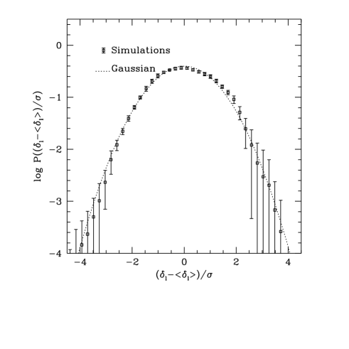
Figure 8: Average reconstructed PDFs. Left panel shows the average reconstructed PDF for ”NOG-unbiased filled with PSCz–unbiased” simulated catalogues. The non-Gaussianity is due to the flattening of high-density peaks. Right panel shows the same PDFs after the correction of peak flattening (with coefficients $c_{1}=1.10$, $c_{2}=5.10$; see table 1). In both panels dotted lines show a Gaussian of zero mean and unit variance.

Figure 9: Scatter-plot of true and reconstructed linear densities for one of the simulated catalogues (NOG unbiased filled with PSCz unbiased), with the best-fit transformation.

Finally, we notice that our procedure is conceptually different from the Gaussianization technique of Weinberg (1992), where a Gaussianity of the PDF is directly forced on a linearly reconstructed density field. We apply our “Gaussianization” procedure only on the high-density peaks (the $\delta<0$ density field is completely untouched) to remove the already analized effect of peak flattening.

3.4 Accuracy of the reconstruction in the Fourier space

Due to the inhomogeneous nature of the smoothing performed on the original catalogues, the initial conditions are not recovered down to a scale which is constant in space. Then, to test the reconstruction in the Fourier space without mixing information from different scales we pad to zero both the true and the reconstructed linear density fields beyond $d_{\rm max}$. We also pad in some cases the ZOA, to test the reconstruction in the region which is not subject to the filling procedure. This padding of course induces some phase correlation at large scales. To be sure that any positive correlation of moduli and phases that we find is due to a true signal, we compare the reconstructed linear density field also with the true one centred in a point which is half the box size away from the centre of the simulated catalogue considered. In this case the reconstructed and true initial conditions are completely independent, and any correlation must be ascribed to the padding procedure. These initial conditions will be referred to as ”random” in the following.

The true, reconstructed and random initial conditions have been FFT-transformed, and the modes $\delta_{\bf k}$ have been compared one by one in terms of modulus $|\delta_{\bf k}|$ and phase $\varphi_{\bf k}$. To quantify the agreement the modes have been binned into intervals of $k$, and for each bin the following statistics have been computed:

$$S_{\rm module} = \sqrt{\left\langle\left[\frac{|\delta_{\bf k}^{\rm sim}|^{2}-|\delta_{\bf k}^{\rm rec}|^{2}}{P^{\rm sim}(k)}\right]^{2}\right\rangle}$$ (21)

$$S_{\rm phase} = \langle(\varphi_{\bf k}^{\rm sim}-\varphi_{\bf k}^{\rm rec})^{2}\rangle$$ (22)

Figure 10 shows as an example these statistics for the unbiased NOG catalogues filled with unbiased PSCz’s. The curves are averages of the statistics over the ten realizations, the 1-$\sigma$ scatter is also shown. Cross points refer to the comparison of true and reconstructed fields, square points to the comparison of random and reconstructed ones. The thick lines show the expectation for two completely uncorrelated fields, which for $S_{\rm module}$ is:

$$\begin{array}[]{lcl}S_{\rm module}^{\rm uncor}&=&2\frac{(P^{\rm sim}(k)^{2}+P^{\rm rec}(k)^{2}-P^{\rm sim}(k)P^{\rm rec}(k))}{P^{\rm sim}(k)^{2}}\\ \\ &\simeq&2\left[\left(1-\exp^{-k^{2}R^{2}}\right)^{2}+\exp^{-k^{2}R^{2}}\right]\\ \end{array}$$ (23)

(the last passage is done assuming $P^{\rm rec}\simeq P^{\rm sim}\exp^{-k^{2}R^{2}}$, which is approximately true). For the phases we obtain:

$$\begin{array}[]{lcl}S_{\rm phase}^{\rm uncor}&=&\int d\phi_{1}\int d\phi_{2}\frac{1}{2\pi^{2}}(\phi_{1}-\phi_{2})^{2}\\ \\ &\simeq&103.92\\ \end{array}$$ (24)

The integral is computed taking into account that $-\pi\leq(\phi_{1}-\phi_{2})\leq\pi$.

The first statistics quantifies the correlation of the fluctuations of the modules of the modes around the average value (i.e. the power spectrum), the second statistics quantifies the correlation of phases. From figure 10 it is clear that both phases and fluctuations of modules are significantly reconstructed at large scales, while the correlation tends to the random value at large $k$-values. The transition happens at a $k$-value similar to $1/R$, so that in this case the worsening of the agreement is mostly due to smoothing. Finally, phases are apparently reconstructed more accurately than the fluctuations of the modules.

Figure 10: Statistic of reconstruction. The left panel shows $S_{\rm module}$. The right panel shows $S_{\rm phase}$. The curves are averages of the statistics over the ten realizations. Cross points refer to the comparison of true and reconstructed fields, square points to the comparison of random and reconstructed ones. Continuous lines represent the 1-$\sigma$ scatter from the average value for the comparison of true and reconstructed fields, dashed lines for the comparison of random and reconstructed ones. The thick lines show the expectation value of the statistics.

It is important to quantify the $k$-value at which the correlation is lost. We have tried many possible definitions for this $k_{\rm lim}$ quantity, mostly based on the agreement between the phases, which we consider more important than the fluctuations of the modules. Namely, we have defined $k_{\rm lim}$ as the value at which the correlated curve is for the first time within (or for the last time beyond) 2$\sigma$ of the uncorrelated curve, with $\sigma$ that relative of either of the two curves, or the value at which the average correlated curve is at a fixed fraction (say 90 per cent) of the value relative to uncorrelated fields (equation 24). All these definitions give similar values for $k_{\rm lim}$. In particular, the last definition is the most stable one, as it is not based on the noisy curves relative to the scatter. In the following only the results based on the last definition will be presented.

Table 4: Results for $k_{lim}$; $d_{max}=60Mpc/h$

Catalogues	$R_{\rm max}(Mpc/h)$	$k_{\rm lim}(h/Mpc)$	$k_{\rm lim}R_{\rm max}$	$k_{\rm lim}(h/Mpc)$	$k_{\rm lim}R_{\rm max}$
				ZOA padded	ZOA padded
PSCz unbiased	5.99	0.36	2.16	–	–
PSCz biased	5.99	0.37	2.22	–	–
NOG unbiased	5.57	0.38	2.12	–	–
NOG biased	5.57	0.38	2.12	–	–
NOG unbiased filled
with PSCz unbiased	5.57	0.37	2.06	0.37	2.06
NOG unbiased filled
with PSCz biased	5.57	0.36	2.01	0.37	2.06
NOG biased filled
with PSCz unbiased	5.57	0.34	1.89	0.36	2.01

Table 5: Results for $k_{lim}$; $d_{max}=30Mpc/h$

Catalogues	$R_{\rm max}(Mpc/h$	$k_{\rm lim}(h/Mpc)$	$k_{\rm lim}R_{\rm max}$	$k_{\rm lim}(h/Mpc)$	$k_{\rm lim}R_{\rm max}$
				ZOA padded	ZOA padded
PSCz unbiased	3.83	0.38	1.45	–	–
PSCz biased	3.83	0.40	1.53	–	–
NOG unbiased	3.17	0.41	1.30	–	–
NOG biased	3.17	0.41	1.30	–	–
NOG unbiased filled
with PSCz unbiased	3.17	0.38	1.20	0.40	1.27
NOG unbiased filled
with PSCz biased	3.17	0.38	1.20	0.38	1.20
NOG biased filled
with PSCz unbiased	3.17	0.38	1.20	0.38	1.20

Table 4 and 5 give the resulting $k_{\rm lim}$ for the seven sets of simulated catalogues, the two choices of $d_{\rm max}$ and $R_{\rm max}$ and the two cases of no padding or padding of the ZOA. For reference, we give also the quantity $k_{\rm lim}R_{\rm max}$, which is a good indicator of the goodness of the reconstruction. We conclude that: (i) for $d_{\rm max}=60$ $h^{-1}\ Mpc$ the reconstruction is valid up to $k_{\rm lim}R_{\rm max}\simeq 2$, i.e. at scales as small as half of the (Gaussian) smoothing radius; (ii) in the ideal case of no ZOA and no bias, the denser sampling of NOG with respect to PSCz gives a tiny improvement to the reconstruction in terms of $k_{\rm lim}$, with a decreasing $k_{\rm lim}R_{\rm max}$; (iii) the correction of the ZOA makes the advantage of NOG almost vanish; (iv) the gain in $k_{\rm lim}$ obtained by smoothing at a smaller scale (with $d_{\rm max}=30$ $h^{-1}\ Mpc$) is modest, corresponding to a decrease of $k_{\rm lim}R_{\rm max}$, which confirms that scales smaller than $\simeq$ 5 $h^{-1}\ Mpc$ are dominated by highly non-linear dynamics; (v) in the case of biased catalogues the reconstruction works to a smaller $k_{\rm lim}$ value, because the onset of non-linearity is anticipated, while the opposite is true in the case of antibiased catalogues.

3.5 The distribution of the phases

It is useful to check the Gaussianity of the reconstructed initial conditions directly in terms of distribution of the phases.

Figure 11: Distribution of the phases of true (dotted lines) and reconstructed (continuous lines) initial conditions for $k<k_{\rm lim}$. The distributions are averages over 10 simulated catalogues. We show the case for unbiased NOG catalogues filled with unbiased PSCz.

Figure 11 shows, for the unbiased NOG catalogues filled with unbiased PSCz, the average distribution of phases for $k<k_{\rm lim}$, together with the average distribution of the phases of the true initial conditions padded beyond $d_{\rm max}$. We have checked that both distributions are consistent with flat by FFT-transforming them and comparing their spectrum with a white-noise one. We conclude that the flatness of the distribution of the reconstructed phases is preserved by the reconstruction. The same conclusions hold for the other cases.

3.6 Correction of the power spectrum for smoothing

Figure 12 shows the power spectra of the padded true, padded true smoothed (over $R_{\rm max}$) and reconstructed initial density fields averaged over the ten realizations in the case of unbiased NOG catalogues filled with unbiased PSCz. The reconstructed power spectrum is similar to the smoothed one, confirming that the adaptive smoothing scheme adopted by ZTRACE is very similar to smoothing in the (Lagrangian) space of initial conditions. Similar results are obtained in other cases. However, the small discrepancies visible in the figure and present also in the other cases are sometimes larger than the typical error associated to the power spectrum (i.e. the rms over the ten realizations).

To restore the power lost by smoothing, it is possible as a first approximation to simply multiply the FFT-transformed field by the inverse of the Gaussian smoothing kernel, i.e. by $\exp[(kR_{\rm max})^{2}/2]$. This turns out to be a good approximation for the two NOG catalogues. In the PSCz case the correction is improved by multiplying the Gaussian kernel by the ratio of the reconstructed and true (smoothed) padded power spectra, as those shown in figure 12. To check the accuracy of these corrections we discard from the FFT-transformed reconstructions all the modes with $k>k_{\rm lim}$. The density fields are then completed with Gaussian random fields with power spectra truncated below $k_{\rm lim}$. The so-completed fields are then transformed them back to the real space, padded beyond $d_{\rm max}$ and FFT-transformed again to compute the power spectra. We obtain smooth spectra in all the three cases, without any jump at $k_{\rm lim}$.

Figure 12: Power spectra. Dashed line refers to the spectrum of true padded initial density field; dotted line refers to the spectrum of true padded initial density field smoothed over 6 $Mpc/h$; continuous line refers to the average spectrum of reconstructed initial density fields over 10 simulated catalogues. We show the case for unbiased NOG catalogues filled with unbiased PSCz.

4 Results

The three catalogues (PSCz and the two NOG completions with either $b_{\rm rel}=1$ or 1.2) have been processed as described in section 3; for sake of clarity we sum up the procedure again. (i) The relaxed groups have been collapsed to spheroids; (ii) the catalogues have been adaptively smoothed, with reference smoothing radius kept constant within either 60 or 30 $h^{-1}\ Mpc$; (iii) the density fields have been processed by ZTRACE to generate the initial conditions; (iv) the flattening of the peaks has been fixed as described in section 3.3; (v) the power lost by smoothing has been restored as described in section 3.6.

4.1 The PDF of the initial conditions from the NOG catalogue

It is interesting to check the Gaussianity of the initial conditions reconstructed from the NOG catalogue, as done by Monaco et al. (2000) for the PSCz.

Figure 13: Reconstructed PDFs. The upper panels (a,b) show the reconstructed PDFs for the NOG catalogues filled assuming $b_{\rm rel}=1.2$ (continuous line) compared with the average PDFs computed from the biased NOG catalogues filled with unbiased PSCz simulated catalogues (points with errorbars). The left panel (a) shows the case for $d_{\rm max}=60$ $h^{-1}\ Mpc$, the right panel (b) shows the case for $d_{\rm max}=30$ $h^{-1}\ Mpc$. The lower panels (c,d) show the reconstructed PDFs for the NOG catalogues filled assuming $b_{\rm rel}=1$ (continuous line) compared with the average PDFs computed from the unbiased NOG catalogues filled with unbiased PSCz simulated catalogues (points with errorbars). The left panel (c) shows the case for $d_{\rm max}=60$ $h^{-1}\ Mpc$, the right panel (d) shows the case for $d_{\rm max}=30$ $h^{-1}\ Mpc$. Dotted lines show a Gaussian with zero mean and unit variance. In each panel the residuals of the reconstructed PDFs with respect to that of simulations, rescaled to the variance among the simulations, are shown below.

Figure 13 shows the reconstructed PDFs for the two NOG catalogues (filled assuming either $b_{\rm rel}=1$ or 1.2) for $d_{\rm max}=30$ or 60 $h^{-1}\ Mpc$; at this stage the flattening of the peaks and the restoration of power lost by smoothing have not been applied yet. The curves are compared with the average PDFs computed from the simulated catalogues. Consistently with Monaco et al. (2000), no distortion of the PDF is detected beyond that induced by ZTRACE. There is a small discrepancy at $\delta\sim 0$, but it is valid only for one or at most two points, and does not resemble any of the patterns induced by realistic bias schemes (see Monaco et al. 2000); we do not consider this feature as significant.

Figure 14: Distribution of the phases of reconstructed initial conditions for the two completions of NOG (continuous lines), compared with the initial condition from one simulated catalogue (dotted lines). Fields are padded to zero beyond $d_{\rm max}=60$ $h^{-1}\ Mpc$. Right panel refers to the case $b_{\rm rel}=1$, left panel refers to the case $b_{\rm rel}=1.2$.

Finally, figure 14 shows the phase distribution of the two sets of initial conditions padded to zero beyond $d_{\rm max}=60$ $h^{-1}\ Mpc$, for $k<k_{\rm lim}$, where $k_{\rm lim}$ is taken from the corresponding case of table 4. For sake of comparison we show also the phase distribution of the initial conditions padded beyond $d_{\rm max}$ for one of the simulated catalogue centres. It is apparent that the weak difference from flatness of the reconstructed phases is consistent with it being an effect of padding (see also figure 11). A similar result holds for the PSCz reconstruction.

4.2 Simulations of the local Universe

The three reconstructions of the initial conditions of our local Universe have been fixed for flattened peaks, as described in section 3.3, and for smoothing, as described in section 3.6. They have then been FFT-transformed and truncated at $k_{\rm lim}$. Finally, the modes at $k>k_{\rm lim}$ have been extracted assuming a $\Lambda$CDM power spectrum with the parameters given in section 3.1 and random phases.

The so obtained density field can be used to generate displacements for a set of particles, so as to produce initial conditions for a constrained N-body simulation of our local Universe. A more refined way to do it relies on the Hoffmann & Ribak (1991, 1992) approach to generate constrained realizations. This would produce a Gaussian density field that is not oversmoothed at large distances. However, in a multi-grid simulation the density field at large distance would anyway be sampled by rather massive particles, thus removing the intermediate scale recovered by the Hoffmann-Riback method.

A comparison of a full-blown simulation with the properties of our local Universe, like the analysis of Narayanan et al. (2001), would require a careful assessment of the bias relation between dark matter and galaxies, and is considered beyond the scope of this paper. However, to perform a “quick and dirty” check of the goodness of the reconstruction, we follow the evolution of 30 different realizations of the initial field (ten for each different reconstructed catalogue) using the PINOCCHIO tool, recently proposed by Monaco et al. (2002). This gives a very fast and accurate approximation of the final distribution of dark matter halos in terms of masses, positions, velocities and merger histories, and has the advantage of running in a very short time compared to a standard N-body code. We are interested in the reconstruction of the large-scale structure, so high resolution is not required for this test. For this reason we run PINOCCHIO on 128³ grids, for a mass resolution of $\sim 10^{12}\ M_{\odot}$ ($h=0.7$). In this case, the smallest reliable halo reconstructed by PINOCCHIO (as well as by an equivalent simulation) is as massive as $\sim 3-5\times 10^{13}\ M_{\odot}$; this mass scale is still dominated by the small-scale power which is randomly added to the ZTRACE reconstruction.

Figure 15: Reconstruction of structures along (left panels) and perpendicular (right panels) to the supergalactic plane. Upper panels show 3 realizations based on NOG with $b_{\rm rel}=1.2$; mid panels show 3 realizations based on NOG with $b_{\rm rel}=1$; lower panels show 3 realizations based on PSCz. Stars indicate halos more massive than $4\times 10^{13}\ M_{\odot}$.

Figure 16: Observed structures along the supergalactic plane. Panel show the location of NOG galaxies.

Figure 15 shows the reconstruction of the NOG volume along the super-galactic plane. Upper panels show 3 realizations based on the NOG catalogue with $b_{rel}=1.2$; mid panels show the same for $b_{rel}=1.2$; lower panels show the same for the PSCz catalogue. Stars indicate the positions of halos reconstructed by PINOCCHIO, with mass grater than $8\times 10^{13}$. For sake of comparison we report in figure 16 the location of NOG galaxies. The main structures observed in the supergalactic plane are correctly reconstructed. In particular, we find that the locations of the main neighbour clusters, like Virgo, Perseus, Pisces, Centaurus and Hydra, are recovered in most if not all cases within a few $h^{-1}\ Mpc$. We have also checked that the sheet-like overdensity corresponding to the supergalactic plane is well reproduced. We find that, as expected, the NOG reconstruction is better than PSCz at high galactic latitude, while it is worse in the optical ZOA.

We conclude that the two catalogues provide comparable reconstructions of the local Universe.

5 Summary and Conclusions

In this paper we have applied the ZTRACE algorithm (Monaco & Efstathiou, 1999) to the NOG (Giuricin et al., 2000) and PSCz (Saunders et al. 2000) catalogues to reconstruct the initial condition of our Local Universe. The use of two different catalogues allows us to test and improve the reconstruction; in particular, the optical catalogue presents the advantages of denser sampling and better relation between optical light and galaxy mass, while the infra-red catalogue benefits from more homogeneous selections and larger sky coverage.

We have studied the relative bias between these catalogues, finding a good linear relation between the density fields traced by them, corresponding to a relative bias of $b_{\rm rel}=1.1\pm 0.1$, in agreement with the expectation based on the ratio of the $\sigma_{8}$ parameters for optical and infra-red galaxies. The scatter around this relation is found to be larger than that implied by shot noise. This may be a sign of stochastic bias; in this hypothesis we obtain a value $\sim 0.25$ for the parameter $\sigma_{b}$ defined by Dekel & Lahav (1999).

We have quantified the accuracy of the reconstruction through extensive testing with simulated galaxy catalogues. The analysis has been performed in the Fourier space. The initial conditions reconstructed by ZTRACE reproduce on large scales both the fluctuations of the modules of the Fourier modes around the mean (the power spectrum) and their phases. The accuracy of the reconstruction drops at a scale corresponding to $k_{\rm lim}\simeq 0.4\ h/Mpc$, beyond which all information is lost. This $k_{\rm lim}$ depends only weakly on catalogue, bias scheme, filling of the ZOA and smoothing scale. In particular, while for a smoothing radius of $\sim 5-6$ $h^{-1}\ Mpc$ the loss of information is determined mainly by smoothing, the reconstruction at smaller scales is limited by non-linearity. Moreover, the denser sampling of the NOG catalogue gives only a modest improvement to the reconstruction, which is anyway compensated by the errors induced by the procedure to fill the ZOA.

Consistently with the PSCz case (Monaco et al. 2000), the initial conditions of the NOG catalogue are found to be consistent with the Gaussian, with no convincing distortion beyond the flattening of the high peaks induced by ZTRACE. We have also checked the distribution of the phases, which is found to be consistent with a uniform one both for PSCz and NOG.

The reconstructed initial conditions have been corrected for smoothing and peak flattening, using corrections calibrated on the simulated catalogues. From these we have generated sets of initial conditions suitable for N-body simulations by randomly generating the modes beyond $k_{\rm lim}$ with a power spectrum given by the cosmology in section 3.1. We have used the PINOCCHIO tool to run three sets of 10 low-resolution simulations, one set from the PSCz and two sets for the NOG (with the ZOA filled assuming two different values for the relative bias between NOG and PSCz, namely $b_{\rm rel}=1$ and 1.2). In all cases the large-scale structure observed in our local Universe is correctly reproduced. The locations of the main neighbouring clusters are also reproduced within a few $h^{-1}\ Mpc$. We notice that the NOG-based realizations are more accurate than PSCz at high galactic latitude, while the opposite is true when the optical ZOA is approached.

With respect to previous works, we improve in many regards. We use different galaxy catalogues, NOG and PSCz, in place of the smaller 1.2 Jy one (Fisher et al. 1995), used by Kolatt et al. (1996) and Mathis et al. (2002); Klypin et al. (2001) used the MARK III catalogue of peculiar velocities (Willick et al., 1997), which allows a reconstruction based on linear theory, but at the cost of a much noisier set of data. Moreover, we use ZTRACE to self-consistently obtain the initial density field from the redshift-space catalogues, and then correct for peak flattening and smoothing with procedures carefully calibrated on simulations.

References

- [] Bertschinger E., 2001, ApJ, 137, 1
- [] Branchini E., Carlberg R.G., 1994, ApJ, 434, 37
- [] Branchini E., Teodoro L., Frenk C.S. et al., 1999, MNRAS, 308, 1
- [] Canavezes A., et al., 1998, MNRAS, 297, 777
- [] Coles P., Sahni V., 1996, 19960bs, 116, 25
- [] Croft R.A.C., Gatzañaga E., 1997, MNRAS, 285, 793
- [] Davis M., Peebles P.J.E., 1983, ApJ, 267, 465
- [] Fisher K.B., Huchra J.P., Davis M. et al., 1995, ApJS, 100,69
- [] Frisch U., Matarrese S., Mohayaee R., Sobolevski A., 2002, Nature, 417, 260
- [] Garcia A.M., 1993, A&AS, 100, 47
- [] Girardi M., Giuricin G., 2000, ApJ, 540, 45
- [] Girardi M., Manzato P., Mezzetti M., Giuricin G., Limboz F., ApJ, 569, 720
- [] Giuricin G., Marinoni C., Ceriani L., Pisani A., 2000, ApJ, 543, 178
- [] Giuricin G., Samurovic S., Girardi M., Mezzetti M., Marinoni C., 2001, ApJ, 554, 857
- [] Gramann M., Cen R., Gott J.R., 1994, ApJ, 425, 382
- [] Hoffman Y., Ribak E., 1991, ApJ, 380L, 5
- [] Hoffman Y., Ribak E., 1992, ApJ,396,448
- [] Huchra J.P., Geller M.J., 1982, ApJ, 257, 423
- [] Joint IRAS Science Working Group, 1988, IRAS Point Source Catalogue, Version 2. US Government Printing Office, Washington DC
- [] Klypin A., Hoffman Y., Kravtsov A.V., Gottlober S., submitted (astro-ph/0107104)
- [] Kolatt T., Dekel A., Ganon G., Willick, J.A. 1996, ApJ, 458, 419
- [] Marinoni C., Monaco P., Giuricin G., Costantini B., 1999, ApJ, 521, 50
- [] Marinoni C., PhD thesis, 2000 (http://astron.berkeley.edu/ m̃arinoni/Thesis/tesibe.ps)
- [] Marinoni C., Hudson M.J., Giuricin G., 2002, ApJ, 569, 91
- [] Materne J., 1978, AUS, 79, 93
- [] Mathis H., Lemson G., Springel V.et al., 2002, MNRAS, 333, 739
- [] Monaco P. & Efstathiou G., 1999, MNRAS, 308, 763
- [] Monaco P., Efstathiou G., Maddox S.J., 2000, MNRAS, 318, 681
- [] Monaco P., Theuns T., Taffoni G., 2002, MNRAS, 331, 587
- [] Narayanan K.V., Croft R.A.C., 1999, ApJ, 515, 471
- [] Narayanan K.V., Weinberg D.H., Branchini E., Frenk C.S., Maddox S., Oliver S., Rowan-Robinson M., Saunders W., 2001, ApJS, 136, 1
- [] Nusser A., Dekel A., 1992, ApJ, 391, 443
- [] Nusser A., Dekel A., Yahil A., 1995, ApJ, 449, 439
- [] Nusser A., Branchini E., 2000, MNRAS, 313, 587
- [] Paturel G. et. al., 1997, A&AS, 124, 109
- [] Peebles P.J.E., 1989, ApJ, 344L, 53
- [] Peebles P.J.E., 1990, ApJ, 362, 1
- [] Rowan-Robinson M., Saunders W., Lawrence A., Leech K., 1991, MNRAS, 253, 485
- [] Saunders W., Sutherland W.J., Maddox S.J. et al., 2000, MNRAS, 317, 55
- [] Saunders W., Rowan-Robinson M., Lawrence A. et al., 1990, MNRAS, 242, 318
- [] Santiago B.X., Strauss M.A., Lahav O. et al., 1995, ApJ, 446, 457
- [] Seaborne M.D. et al., 1999, MNRAS, 309, 89
- [] Somerville R., Lemson G., Sigad Y., Dekel A., Kauffmann G., White S.D.M., 2001, MNRAS, 320, 289
- [] Springel V., Yoshida Y., White M., 2001, NewA, 6, 79
- [] Strauss M.A. & Willick J.A., 1995, Physics Reports, 261, 271
- [] Sutherland W. et al., 1999, MNRAS, 308, 289
- [] Szalay A.S., Jain B., Matsubara T. et al., submitted (astro-ph 0107419)
- [] Taffoni G., Theuns T., Monaco P., 2002 MNRAS, 333, 623
- [] Tully R.B., Nearby galaxies catalog, Cambridge University Press, 1988
- [] Weinberg D.H., 1992, MNRAS, 254, 315
- [] Willick J.A., Courteau S., Faber S.M. et al., 1997, ApJS, 109, 333
- [] Zel’dovich Y.B., Shandarin S.F., Rev. Mod. Phys., Vol 61, No. 2, April 1989