Blobby accretion in magnetic cataclysmic variables

Abstract

The processes of accretion of the gaseous blobs with different masses and densities onto strongly magnetized white dwarfs in the systems of polars have been modeled. We have proved that shot noise in blue wavelengths represents accretion of the smaller and denser blobs than in redder wavelengths. Using combined ”smooth particle hydrodynamics - drag force” model, we have predicted a shape of the accretion stream and active regions on the white dwarf surface.

Department of Astronomy, Odessa National University, T.G.Shevchenko park, 65014, Odessa, Ukraine, halevin@astronomy.org.ua

Crimean Astrophysical Observatory, Nauchny 98409 Crimea, Ukraine

Astronomical Observatory, Odessa National University, T.G.Shevchenko park, 65014, Odessa, Ukraine

1. Introduction

The idea about the blobby accretion in magnetic cataclysmic variables had appeared as an attempt to explain the flickering and the soft X-ray excess in such systems. The fast variability at a time-scale of dozens of seconds is well described by the “shot noise” model with an exponential decay of its auto-correlation function (ACF, Andronov 1994). The “shot noise” is interpreted as a result of accretion of large diamagnetic blobs (Beardmore & Osborne 1997; Kuijpers & Pringle 1982; Panek 1980).

Such blobs originate due to the Rayleigh-Taylor instabilities, when a heavy fluid (matter) is opposed in the gravitation field to a light fluid (magnetic field).

The dynamical properties of such blobs were investigated by King (1993). The drag force, which has an influence on the trajectories of the blobs in magnetic field is expressed as follows:

$$f_{drag}=-k[\vec{\nu}^{\prime}-(\vec{\nu}^{\prime}\cdot\vec{b}^{\prime})\vec{b}^{\prime}]$$ (1)

The drag coefficient

$$k=\frac{B^{2}l^{2}}{c_{A}m}$$ (2)

is dependent on such parameters, as the magnetic field strength $B$, blob size $l$, blob mass $m$ and Alfvén velocity in interblob plasma $c_{A}$. Because the Alfvén velocity and the mass of the blob are expressed as

$$c_{A}=\frac{B}{\sqrt{4\pi\rho_{i}}},~{}~{}~{}m=\frac{4}{3}\pi l^{3}\rho_{b}$$ (3)

where $\rho_{b}$ and $\rho_{i}$ are the densities of the blob and interblob plasma in the flow, respectively, the drag coefficient is expressed as

$$k=\frac{3B\rho^{1/2}}{2\pi^{1/2}\rho_{b}l}$$ (4)

In the models of accretion, the dipolar field configuration is usually assumed, although, it is not a precise approach.

Varying the parameters of density and size, we can achieve a good approach to the observations, comparing blob velocities with existing Doppler tomograms (e.g. Heerlein et al. 1999).

Possible differences between the blob parameters, such as mass and size (Wynn & King 1995), could lead the differences in locations of the active regions on the white dwarf surface and in the variability of the shot noise decay time.

If we calculate the blob trajectories with the range of sizes between $10^{8}$ to $10^{10}$ cm, then in the case of HU Aqr, we can obtain the next ideal dependence of the initial blob size on the azimuth on white dwarf surface (Fig.1).

Figure 1.: Dependence of the initial size of the accreted blobs on the longitude at the white dwarf surface.

Having such a clear picture of distribution of the blob sizes at the white dwarf surface, we can expect the smooth variability of the shot noise decay time. If we remove the orbital variability from our observations, we can calculate the biased ACF and, using the method described by Andronov (1994), we can calculate the exponential decay time for unbiased ACF.

During the fall onto the white dwarf’s surface, the blobs are deformed owed to tidal forces. The undisturbed size of a blob is expressed by Halevin et al.(2002b) as

$$l=\frac{\tau}{4}\left(\frac{2GM_{wd}}{r_{coup}}\right)^{1/2}$$ (5)

where $r_{coup}$ is the coupling distance and $M_{wd}$ is a mass of the white dwarf. One can see that the falling time of the blobs does not depend on the stopping height.

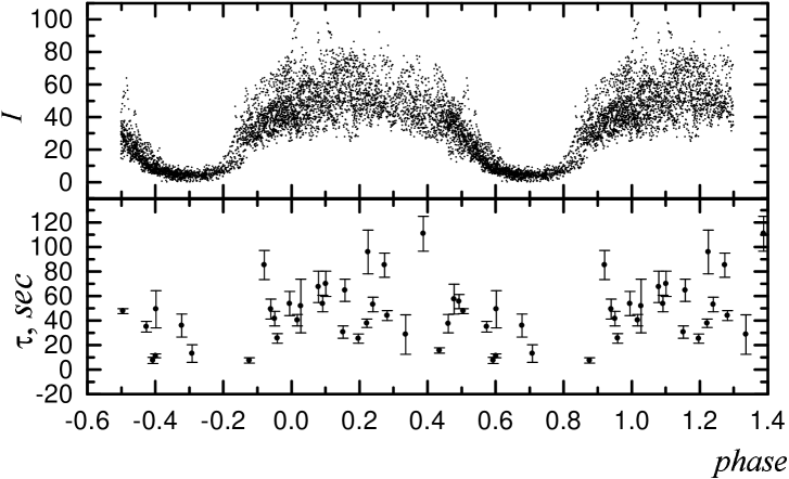
Figure 2.: Phase curves for count rate and $\tau$ for Ginga satellite observations of AM Her. Period is 0.128927041 days (Greeley et al. 1999).

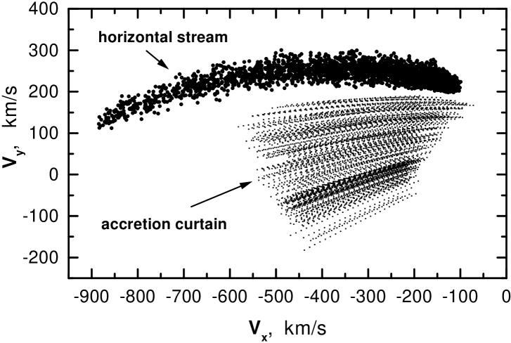
Figure 3.: Positions of the SPH points in velocity space for HU Aqr.

In the Fig.2, one can see the phase variability of the shot noise decay time for X-ray Ginga observations of AM Her. Although the data are significant, we do not see smooth variations, as expected.

To make more realistic model of blobby accretion in polars, we have used the SPH method. The pure hydrodynamical model was made by Cach & Howell (2002). Dynamical positions of the flow points at the Doppler tomogram is shown in Fig.3.

In our model, we have used the hydrodynamical parameters of the flow to make comparison between the gas pressure (not the ram one) and the magnetic pressure. When the magnetic pressure becomes larger than the gas pressure, we convert our SPH points into blobs.

Here we used computed from our model parameters of the flow with the formula of Hameury, King, & Lasota (1986) for the minimum scale of the structures which are unstable to the Rayleigh-Taylor mechanism

$$l=\frac{B^{2}_{b}r^{2}_{b}}{2GM_{wd}\rho_{b}}$$ (6)

where $B_{b}$ is magnetic field and $r_{b}$ is the distance of blob appearance. Substituting (6) to the (4), we obtain the expression for the drag force in the next form:

$$k=\frac{4\pi^{1/2}GM_{wd}B\rho^{1/2}_{i}}{r^{2}_{b}B^{2}_{b}}$$ (7)

The very interesting result is that, under such assumptions, the drag force does not depend neither on the blob sizes nor on the blob density, but only on the magnetic field and the interblob plasma density, which we assumed to be a constant.

The modeled Doppler tomogram for HU Aqr is shown in Fig.4.

Figure 4.: Doppler tomogram for combined SPH-”drag force” model in the case of HU Aqr.

First of all, one can see that this model cannot explain the observed accretion curtain features. It will be possible, if we take into account the disruption of the blobs by the Kelvin-Helmholtz instability. In the next Fig.5, one can see the distribution of the accretion blob sizes on the white dwarf surface for the case of AM Her. There is already no strong dependence. However, possible effect is that large blobs can originate in outer parts of the accretion stream, and, hence, they will fall into outer parts of the active region on white dwarf surface.

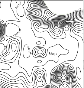
Figure 5.: Initial size (cm) distribution of the accreted blobs on the white dwarf surface in the case of AM Her.

Let analyze again the decay scale variability curves. The composite curves do not show strong dependencies. But some individual curves (as in the case of BY Cam) can show them.

Much more simpler can be the picture for the soft X-ray shot noise, because the source of this radiation is expected have a zero (or about) height.

Take a look at the size distribution (Fig.5). Because the sizes of the blobs are in inverse proportion with the blob density and the density is inversely proportional to the shock height, we can expect that this distribution is about to express also the shock height. Such distribution of the shock heights could explain the observed double humped orbital soft X-ray variability of AM Her (Christian 2000) as absorption by higher shocks.

Under our assumptions, larger blobs have smaller densities. As we know from the work of Fisher & Beuermann (2001), for larger accretion rate per unit area, the maximum of cyclotron radiation shifts to the shorter wavelengths. So we can expect, that in blue wavelengths we can observe accretion of the shorter blobs, that has been already discovered by Beardmore & Osborne (1997).

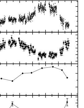
Figure 6.: Phase curves for a magnitude, polarization, shot noise amplitude and $\tau$ for 2.5-m telescope observations of the BY Cam (Halevin et al. 2002a).

So, let me show the final results of investigations of the shot noise decay time in magnetic cataclysmic variables (Table 1). For AM Her and EF Eri, we have analysed the X-ray variability and detected the mean decay times of about 70 s.

Table 1.: Mean decay time estimates.

Star	$\tau$, s	wavelengths	Magn. field, G	ref.∗
AM Her	67.5$\pm$9.2	X-ray, 1.7-10.4 keV	13	H1
AM Her	70	optical I,R bands	13	BO
AM Her	25	optical U band	13	BO
EF Eri	69.0$\pm$11.0	X-ray, 1.7-10.4 keV	16	H1
BY Cam	40.8$\pm$5.1	optical V,R bands	40	H1
QQ Vul	42.8$\pm$5.7	optical V,R bands	35	H2
AR UMa	no shot noise?	optical V,R bands, low state	250	SH

^∗ H1 - Halevin et al. (2002a), H2 - Halevin et al. (2002b), BO - Beardmore & Osborne (1997), SH - Shakhovskoy & Halevin (2000).

From optical observations in V and R band for BY Cam and QQ Vul, the systems with higher magnetic fields, the decay time is smaller. For AR UMa, we could not find the shot noise because the system was in its low state. But it can be the consequence of the high magnetic field and the full disruption of the blobs by the Kelvin-Helmholtz instability.

So, the main our future perspectives are:
$\bullet$Advanced models with Kelvin-Helmholtz disruption.
$\bullet$Investigations of the shot noise behavior in soft X-rays.
$\bullet$Investigations of the systems with different magnetic fields, especially high-field polars.
$\bullet$Analysis of the long term behavior of the shot noise parameters.

References

Andronov, I.L. 1994, Astron.Nachr., 315, 353

Beardmore, A.P., & Osborne, J.P. 1997, MNRAS, 290, 145

Cash, J.L., & Howell, S.B. 2002, ASP Conf Ser. 261, 141

Christian, D.J. 2000, ApJ, 119, 1930

Fisher, A., & Beuermann, K. 2001, A&A, 373, 211

Greeley, B.W., Blair, W.P., Long K.S., & Raymond J.C. 1999, ApJ, 513, 491

Halevin, A.V., Andronov, I.L., Shakhovskoy, N.M., Pavlenko, E.P., Ostrova, N.I. & Kolesnikov, A.V. 2002a, ASP Conf Ser. 261, 155

Halevin, A.V., Shakhovskoy, N.M., Andronov, I.L., & Kolesnikov, A.V. 2002b, A&A, 394, 171

Hameury, J.-M., King, A.R., & Lasota, J.-P. 1986, MNRAS, 218, 695

Heerlein, C., Horne, K., & Schwope, A.D. 1999, MNRAS, 304, 145

King, A.R. 1993, MNRAS, 261, 144

Kuijpers, J., & Pringle, J.E. 1982, A&A, 114, L4

Panek, R.J. 1980, ApJ, 241, 1077

Shakhovskoy, N.M., & Halevin, A.V. 2000, IBVS No. 4858

Wynn, G.A., & King, A.R. 1995, MNRAS, 275, 9