A New approach for a Galactic Synchrotron Polarized Emission Template in the Microwave Range

Abstract

We present a new approach in modelling the polarized Galactic synchrotron emission in the microwave range (20-100 GHz), where this radiation is expected to play the leading role in contaminating the Cosmic Microwave Background (CMB) data. Our method is based on real surveys and aims at providing the real spatial distributions of both polarized intensity and polarization angles. Its main features are the modelling of a polarization horizon to determine the polarized intensity and the use of starlight optical data to model the polarization angle pattern. Our results are consistent with several existing data, and our template is virtually free from Faraday rotation effects as required at frequencies in the cosmological window.

1 Introduction

The polarized component of the diffuse background emission in the microwave range is of great interest for both the Galactic structure and the CMB. Actually, its measurement leads to probing the structure of the interstellar medium (ISM) and the Galactic magnetic field. Moreover, the detection of CMB Polarization (CMBP) allows the investigation of the early Universe.

CMB anisotropies and polarization are powerful tools to determine cosmological parameters (Sazhin & Benitez 1995, Zaldarriaga, Spergel & Seljak 1997, Kamionkowski & Kosowsky 1998). However, although anisotropies have been already detected and space missions (MAP, PLANCK) are expected to make all-sky surveys down to $0^{\circ}.1$ angular resolution, CMBP still represents a challenge for astronomers. The first detection has been just claimed by DASI (Kovac et al. 2002) and several experiments will address it soon (SPOrt (see Carretti et al. 2002, Cortiglioni et al. 2002), MAP, PLANCK, B2K2 (Masi et al., 2002), BaR-SPOrt (Zannoni et al., 2002) and AMiBA (Kesteven et al., 2002) among the others).

Besides the CMBP low emission level (3-4 $\mu$K on sub-degree scales and $<1\,\mu$K on large ones), difficulties in its detection are mainly related to the presence of foreground noise from Galactic and extragalactic sources. Extragalactic foregrounds essentially consist of radio and infrared discrete sources, whereas Galactic foregrounds are generated by synchrotron, free-free, thermal dust and spinning/magnetic dust emissions.

Synchrotron polarized emission should represent the most relevant foreground in the microwave range: free-free is fainter ($<4\,\mu$K at 30 GHz in total intensity, see Reynolds & Haffner 2000) and almost unpolarized, whereas thermal dust has a polarization degree much smaller than synchrotron (Prunet et al. 1998, Tegmark et al. 2000). Evidence for spinning or magnetic dust emission has been found (Kogut et al. 1996, de Oliveira–Costa et al., 2002) but it seems to play an important role only up to $\sim 50$ GHz. Moreover, it should have a low polarization degree (Lazarian & Prunet 2002).

In spite of its importance, synchrotron emission is scarcely surveyed: existing data mainly cover the Galactic Plane area at frequencies up to 2.7 GHz, far away from the cosmological window (Duncan et al. 1997, hereafter D97, Duncan et al. 1999, hereafter D99, Uyaniker et al. 1999, Gaensler et al. 2001, Landecker et al. 2002). The Leiden data (Brouw & Spoelstra 1976, hereafter BS76) cover high Galactic latitudes, but are limited to $<$ 1.4 GHz and are largely undersampled. This situation makes having a reliable synchrotron polarized emission template in the 20-100 GHz range very important. This would allow, for instance, reliable numerical simulations to set-up and test destriping techniques or foreground separation methods (Revenu et al. 2000, Sbarra et al. 2003, Tegmark et al. 2000 and references therein). At present, only toy models exist, which do not account for the real spatial distribution of both polarization intensity and polarization angles (Kogut & Hinshaw 2000, Giardino et al. 2002).

In this paper we present a new approach in modelling the Galactic diffuse synchrotron polarized emission in the 20-100 GHz range. It is based on real surveys and fitted to the real spatial distribution of both polarized intensity and polarization angles. Low frequency data are used to model the polarized intensity and optical starlight is used to model polarization angles. This allows the construction of $Q$ and $U$ maps covering about half of the sky with the SPOrt experiment angular resolution (FWHM $=7^{\circ}$). Although our work is finalized to the SPOrt experiment, the method is general enough to be suitable also for smaller angular scales as soon as complete sets of data with sub-degree angular resolution will be available.

The great advantage of this new approach is to produce $Q$ and $U$ maps free from Faraday rotation, allowing a direct extrapolation to the cosmological window.

The outline of the paper is as follows: the synchrotron polarized emission model and the procedure to build the template are presented in Section 2, results and comparisons with existing data are described in Section 3 and 4, respectively, whereas Section 5 contains the conclusions.

2 THE MODEL

2.1 Ingredients

The aim of our work is to generate template maps of the two linear Stokes parameters $Q$ and $U$ of the Galactic synchrotron polarized radiation in the cosmological window near 100 GHz with the SPOrt angular resolution (FWHM $=7^{\circ}$). We divide the problem in two parts:

1. constructing a polarized intensity ($I_{p}$) map: it can be obtained from existing total intensity ($I$) sky surveys assuming a model linking the polarized to the total intensity synchrotron emission;

2. building a map of polarization angles not affected by the effects of Faraday rotation. At present, only optical starlight data fulfil this requirement.

The Haslam map (Haslam et al. 1982) is the most complete sky survey at radio wavelenghts, where synchrotron emission is dominant. It is a full-sky map at $408$ MHz with a resolution of $51$ arcmin obtained combining observations taken with different radiotelescopes. However, it is not perfect for our aims since the free-free emission is still significant, expecially in the Galactic plane (Reich & Reich 1988, hereafter RR88). Consequently, identification and subtraction of this contribution is mandatory. As described in Section 2.2, we perform this separation using the Dodelson (1997) formalism, which requires a second map at different frequency. We use the Reich (1982) map at 1.4 GHz with an angular resolution of $35$ arcmin, the only other available survey with absolute calibration covering a large part of the sky ($\delta\geq-17^{\circ}$).

The polarization angles are taken from the Heiles starlight polarization catalogue (Heiles 2000). These data have many advantages with respect to those in the radio band: they are free from Faraday rotation and they cover almost all the sky. The catalogue lists polarization degree, position angle and distance of about $9000$ stars from both hemispheres. Further properties of this catalogue and considerations confirming its validity as a polarization angle pattern for our model are described in section 2.4.

2.2 Synchrotron Intensity Map

The different frequency behaviour of free-free and synchrotron emissions allows the application of the Dodelson technique (Dodelson 1997) to Haslam (0.408 GHz) and Reich (1.4 GHz) maps. The original Dodelson formalism is centred on the CMB frequency dependence, so that here a slight modification is introduced to adjust the method to the synchrotron–free-free case. For each pixel $i$ a vector ${\bf T}_{i}$ is defined whose elements are the pixel antenna temperatures at the two frequencies. Its expression in terms of synchrotron and free-free components is given by:

$${\bf T}_{i}={\bf{T}}^{s}_{i}+{\bf{T}}^{f\!f}_{i}+{\bf N}_{i},$$ (1)

where ${\bf{T}}^{s}_{i}$ and ${\bf{T}}^{f\!f}_{i}$ are the synchrotron and free-free contributions, respectively, and ${\bf N}_{i}$ is the noise.

Assuming the noise from the two maps is completely uncorrelated (it comes from different experiments), the correlation matrix

$$C_{ab,i}=\left<N_{a,i}N_{b,i}\right>$$ (2)

is diagonal with pixel variances as elements ($a$ and $b$ indicate the frequencies).

Provided the frequency behaviours (shapes) ${\bf{F}}^{s}_{i}$ and ${\bf{F}}^{f\!f}_{i}$ are known, the estimators ${\bf{\Theta}}^{s}_{i}$ and ${\bf{\Theta}}^{f\!f}_{i}$ of ${\bf{T}}^{s}_{i}$ and ${\bf{T}}^{f\!f}_{i}$ can be expressed as:

$${\bf\Theta}^{s}_{i} = \theta^{s}_{i}{\bf{F}}^{s}_{i}$$ (3)

$${\bf{\Theta}}^{f\!f}_{i} = \theta^{f\!f}_{i}{\bf{F}}^{f\!f}_{i}$$ (4)

where $\theta^{s}_{i}$ and $\theta^{f\!f}_{i}$ are the unknown amplitudes of synchrotron and free-free, respectively.

In the range $0.408-1.4$ GHz free-free and synchrotron are known to follow power laws, so that their shapes are

$${F}^{s}_{i,a} = \nu_{a}^{-\beta_{i}}$$ (5)

$${F}^{f\!f}_{i,a} = \nu_{a}^{-\alpha}$$ (6)

with the free-free spectral index $\alpha=2.1$ (RR88). The frequency behaviour of synchrotron radiation depends on the energy distribution of relativistic electrons and is spatially varying across the sky.

We define a scalar product between vectors as

$${\bf R}\cdot{\bf S}=\sigma^{(0)^{2}}_{\theta}\sum^{2}_{a,b=1}R_{a}C^{-1}_{ab}S_{b}.$$ (7)

This expression is similar to that of Dodelson, apart from the normalization factor

$$\sigma^{(0)^{2}}_{\theta}=\frac{1}{\sum^{2}_{a,b=1}F^{f\!f}_{a}F_{b}^{f\!f}C^{-1}_{ab}},$$ (8)

which here is based on the free-free shape rather than on that of CMB. Again following Dodelson, the best estimate of the amplitudes is given by

$$\theta^{s}_{i} = \sum_{j}K^{-1}_{1j}{\bf{F}}^{j}_{i}\cdot{\bf T}_{i},$$ (9)

$$\theta^{f\!f}_{i} = \sum_{j}K^{-1}_{0j}{\bf{F}}^{j}_{i}\cdot{\bf T}_{i}\hskip 28.45274pt\mbox{with }j=s,f\!f,$$ (10)

where the matrix K is defined as

$$K_{ij}={\bf F}^{i}\cdot{\bf F}^{j}.$$ (11)

As a result, the two components are separated providing the two maps of synchrotron ($\theta^{s}_{i}$) and free-free ($\theta^{f\!f}_{i}$).

The spectral index $\beta_{i}$ has been modelled using the analysis of RR88 who compared data at $408$ MHz and $1.4$ GHz obtaining the following results:

• $\beta\sim 2.85$ toward the Galactic anticentre at $b=0^{\circ}$ of Galactic latitude, with a flattening with incresing $z$ ($z$ is the height above the Galactic plane);

• $\beta\sim 3.1$ in the inner disk (Galactocentric distance $<8$ kpc and $|z|<2$ kpc). In this region the spectral index is nearly constant, beginning to decrease from $|b|\simeq 10^{\circ}$ until reaching the value of $\beta\sim 2.65$ at $|b|\simeq 30^{\circ}$;

• $\beta\sim 2.65$ for $|b|>30^{\circ}$ independently of the Galactic longitude $l$.

The transition from the inner disk region to the rest of the Galactic plane occurs between $l=45^{\circ}$ and $l=55^{\circ}$, where a flattening from $\beta=3.1$ to $\beta=2.85$ is observed. From spectral index profiles (cfr. Figure 5 in RR88) we find the linear behaviour to be a good approximation for $\beta$ in the transition regions. From these considerations, we model the distribution of synchrotron spectral indeces as follows (see Figure 1):

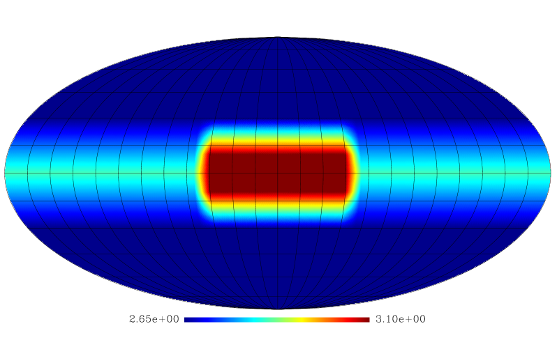
Figure 1: Synchrotron spectral index map in the 0.408–1.4 GHz range (see text and RR88 for details). The map is in Galactic coordinates with the Galactic Centre in the middle and Galactic longitudes increasing toward left.

1) a region towards the Galactic centre ($|b|<10^{\circ}$ and $l<45^{\circ}$, $l>315^{\circ}$) with $\beta=3.1$;

2) a region towards the Galactic anticentre on the Galactic plane ($b=0^{\circ}$ and $55^{\circ}<l<305^{\circ}$) with $\beta=2.85$;

3) a region at high Galactic latitude ($|b|>30^{\circ}$) with $\beta=2.65$.

4) the spectral index follows a linear behaviour in the transition regions and continuity is imposed at borders. Figure 2 shows the spectral index behaviour in three special cases.

Figure 2: Spatial behaviour of the synchrotron spectral index $\beta$ for three special cases: $l=0^{\circ}$ (a), $l=180^{\circ}$ (b) and $b=0^{\circ}$ (c).

2.3 From Total to Polarized Intensity Map

A common result of radio-surveys in polarization is the identification of two main components: a strong emission from discrete sources (Supernova Remnants - SNRs - and several sources with no $I$-counterpart) and a weaker, diffuse emission from a background component (D97, D99, Landecker et al. 2002, Gaensler et al. 2001) that appears to be rather constant with the longitude independently of both angular resolution and frequency. This isotropic background suggests the presence of a polarization horizon, a local screen beyond which the polarized emission is cancelled out (D97, Gaensler at al. 2001, Landecker et al. 2002). The horizon can be imagined as a sort of bubble centred in the observer position (see Figure 3): the net polarized signal is only that integrated along the line of sight out to the horizon, whereas signals beyond the horizon are depolarized by variations of polarization angles (changes and turbulence in the Galactic magnetic field).

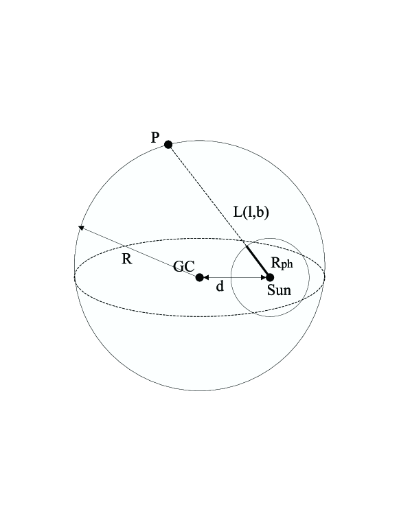
Figure 3: Contributions to the Galactic polarized radiation are limited by a polarization horizon, a local bubble of radius $R_{ph}$ centred on the Sun (see text for details). The thickness $L(l,b)$ of the synchrotron emitting region of our simple spherical model (the distance of the halo point $P$ from the Sun position) is also shown.

A further element suggesting the existence of such a horizon comes from Landecker et al. (2002), who show that only the closest SNRs are well visible also in polarized emission, whereas the most distant ones completely disappear.

The size of the horizon is not yet known: it depends on several effects along the line of sight, like Galactic magnetic field turbulence and electron density variations. However, it has been suggested that it can range from $2$ kpc (Gaensler et al. 2001) up to 7 kpc (D97, Landecker et al. 2002), so that a few kpc appeares to be a quite acceptable estimate.

The polarization horizon allows us to model the relation between polarized and total intensity synchrotron emissions. Given the mean total synchrotron emissivity $J^{s}(\nu,l,b)$ at Galactic coordinates $(l,b)$ and the thickness $L(l,b)$ of the synchrotron emitting region (see Figure 3) in the same direction, the brightness temperature $T^{s}(\nu,l,b)$ at frequency $\nu$ is:

$$T^{s}(\nu,l,b)=\frac{c^{2}}{2K\nu^{2}}J^{s}(\nu,l,b)\,L(l,b),$$ (12)

where $K$ is the Boltzmann constant. The thickness $L(l,b)$ depends on the geometrical model describing the space distribution of the relativistic–electron gas responsible for synchrotron emission. As a first step in modelling the polarized synchrotron radiation we consider the simplest case where the gas is uniformly distributed in the Galactic halo. This is represented by a sphere of radius $R=15$ kpc centred into the Galactic Centre (GC). Thus, in our simple case the line of sight $L(l,b)$ is the distance between the Sun and the edge of this sphere:

$$L(l,b)=d\,\cos(b)\,\cos(l)\,\left[1+\sqrt{1+\frac{(R^{2}/d^{2}-1)}{\cos^{2}(b)\,\cos^{2}(l)}}\right],$$ (13)

where $d=9$ kpc is the Sun distance from GC (See Figure 3 and Appendix A for details).

The polarized brightness temperature $T_{p}^{s}$ can be similarly defined provided the emission is integrated out to the polarization horizon $R_{ph}$ and a polarization degree $p$ is introduced:

$$T^{s}_{p}(\nu,l,b)=\frac{c^{2}}{2K\nu^{2}}\,p\,J^{s}(\nu,l,b)\,R_{ph}.$$ (14)

Finally, equations (12) and (14) provide the relation between polarized and total intesity emissions:

$$T^{s}_{p}(\nu,l,b)=p\frac{R_{ph}}{L(l,b)}T^{s}(\nu,l,b)$$ (15)

The quantity $p\,R_{ph}$ is unknown and represents a free parameter to be calibrated with real data.

2.4 Polarization angle map

The propagation of an electromagnetic wave of wavelength $\lambda$ through a plasma in presence of a magnetic field ${\bf B}$ is affected by Faraday rotation. The net effect is a change in the polarization angle $\phi$ by

$$\Delta\phi = \mbox{RM}\,\lambda^{2}$$ (16)

RM $$= 812\int n_{e}(\mbox{cm}^{-3})\,{\bf B}(\mu\mbox{G})\cdot d{\bf l}({\rm kpc})\,\mbox{rad m}^{2}$$

where RM is the rotation measure, $n_{e}$ is the plasma electron density and $d{\bf l}$ is the infinitesimal path along the line of sight.

Estimates of RM from extragalactic radio sources give typical values ranging from tens to hundreds rad/m² at medium and high Galactic latitudes, and from tens to thousands rad/m² in the Galactic plane (Simard-Normandin & Kronberg 1980, Sofue & Fujimoto 1983, hereafter SF83, Brown & Taylor 2001, hereafter BT01). In particular, the behaviour along the Galactic plane is well fitted by (BT01)

$$\mbox{RM}(l) = \mbox{RM}_{0}\cos(l-l_{0})$$ (17)

$$\mbox{RM}_{0} = -183\pm 14\mbox{ rad/m}^{2}$$

$$l_{0} = 84^{\circ}\pm 4^{\circ}.$$

Brown & Taylor suggest that the modulation in RM occurs because of a local constant magnetic field.

Equation (17) gives, in the frequency range of the cosmological window ($20-100$ GHz), negligible Faraday rotation effects ($\pm 2.5^{\circ}$ at 20 GHz): all we need is a template of intrinsic polarization angles. When used at $2.7$ GHz, which is the highest frequency of present polarization surveys, equation (17) results in angular rotations up to $\pm 160^{\circ}$. This means that radio polarization data cannot be used to build a reliable template of intrinsic polarization angles.

To overcome this problem we use the Heiles catalogue on starlight polarization, the optical frequency being unaffected by Faraday rotation.

The polarization vector of starlight is parallel to the Galactic magnetic field $\bf B$ because of selective absorption by interstellar dust grains, whose minor axis is aligned with $\bf B$ (Fosalba et al., 2001). Since the synchrotron polarization vector is perpendicular to $\bf B$, starlight polarization angles can be used as a template provided a $90^{\circ}$ rotation is performed.

Most of the Heiles catalogue stars ($\simeq 87\%$) are within $2$ kpc (see Figure 4), tracking the local magnetic field. Their distance is in the order of the polarization horizon size (see Section 2.3) confirming that the Heiles catalogue can be safely used as a template for the polarization angles of synchrotron emission. The main problems to face with when using Heiles polarization angles are the irregular distribution of data and the variable sampling distance. However, if the uniformity scale of the angles is compatible with the sampling distance of the catalogue, the lack of data can be filled by linear interpolation.

An estimate of the uniformity scale can be obtained from Figures 9 and 10 of D97, showing that background emission regions have a polarization angle pattern varying slowly on scales of $5^{\circ}-10^{\circ}$. Only areas with strong sources show a more complex structure, but their modellization is out of the purposes of this paper.

The sampling distance of the Heiles catalogue (Figure 6) is compatible with the uniformity scale everywhere but in the region centred in ($l=135^{\circ},b=40^{\circ}$) where it is greater than $10^{\circ}$. We exclude this region from the interpolation procedure as well as from final template maps.

We perform the interpolation by generating $Q$, $U$ pairs corresponding to the Heiles polarization angles $\theta$:

$$Q_{\theta} = \cos\,(2\theta);$$ (18)

$$U_{\theta} = \sin\,(2\theta).$$ (19)

Then, for each pixel of the template map under construction we linearly interpolate the $Q_{\theta}$ and $U_{\theta}$ values of the three closest stars and compute the corresponding polarization angle. The interpolation methods uses parallel transport as described in Bruscoli et al. (2002).

Figure 4: Number of Heiles stars versus Sun distance.

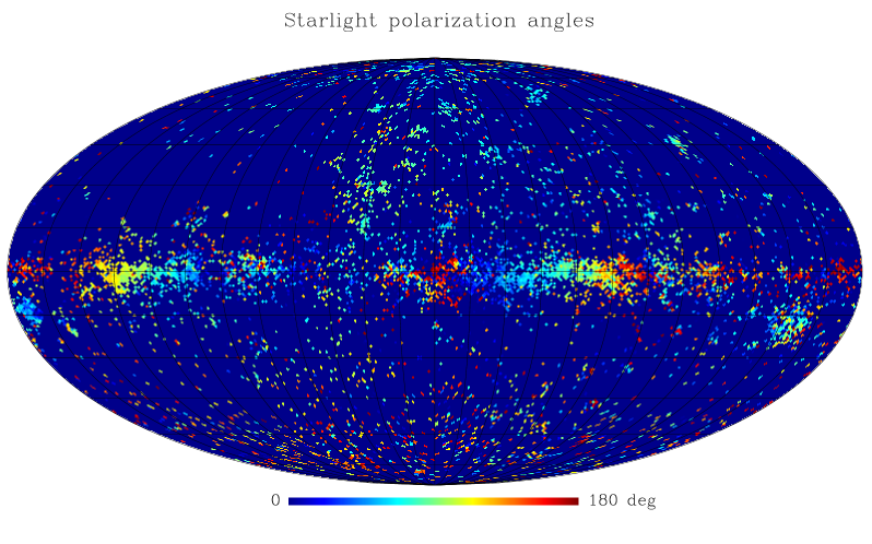
Figure 5: Polarization angles of stars in the Heiles catalogue (degrees): each star is represented by a pixel in a HEALPix format map with $Nside=128$ (pixel size $\simeq 0^{\circ}.5$)). The map is in Galactic coordinates.

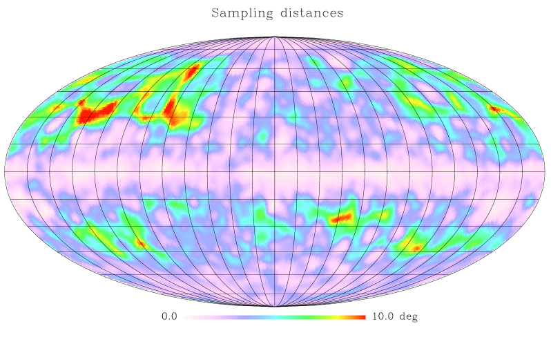
Figure 6: Map of sampling distances (degrees) of the Heiles catalogue. The map is in Galactic coordinates.

2.5 The Procedure

The polarized synchrotron emission template is built as follows:

1. the CMB emission and the absolute calibration error are removed from both the Reich and the Haslam maps using values suggested in RR88 ($3.7$ K and $2.8$ K for Haslam and Reich maps, respectively);

2. the resulting maps are resampled in HEALPix format with $N_{side}=128$, corresponding to a pixel size of about half a degree;

3. Reich map data are smoothed to the Haslam resolution (FWHM $=51$ arcmin);

4. the technique for component separation described in Section 2.2 is applied by using the synchrotron spectral index pattern previously described. This results in the $I$ synchrotron emission map;

5. the relation between $I$ and $I_{p}$ described by equation (15), which introduces the effects of the polarization horizon, is used to provide the shape of the $I_{p}$ map, the parameter $p\,R_{ph}$ being still free. Its calibration is performed a posteriori on BS76 data and a detailed discussion is presented in Section 3;

6. from the $I_{p}$ map and from the angle map obtained from starlight data, $Q$ and $U$ maps are computed;

7. the $Q$ and $U$ maps produced in this way are convolved with a FWHM $=7^{\circ}$ Gaussian filter to match the SPOrt angular resolution. The smoothing procedure applies the parallel transport method described in Bruscoli et al. (2002)

3 The Polarized Synchrotron Template

Our results are shown in Figure 7, where the $Q$ & $U$ templates at 1.4 GHz are presented. Figure 8 shows a comparison between the polarized intensity $I_{p}$ of our model and the $I_{p}$ map obtained from BS76 data. The comparison is performed only for $I_{p}$ because polarization angles are strongly affected by Faraday rotation at 1.4 GHz (see Section 2.4).

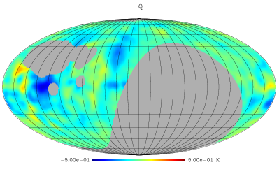
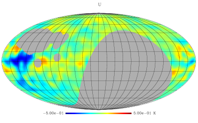
Figure 7: $Q$ (left) and $U$ (right) maps of our synchrotron polarized emission template (Kelvin). The maps are at 1.4 GHz convolved with a FWHM$=7^{\circ}$ Gaussian filter.

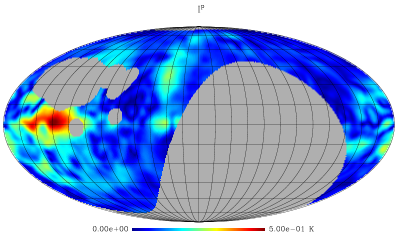
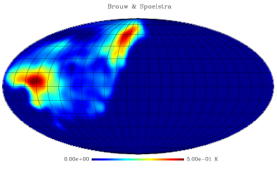
Figure 8: Same of Figure 7 but for $I_{p}$. Our template (left) is compared with 1.4 GHz BS76 data (right).

Areas not covered by our template are in grey: they correspond to the Southern sky not surveyed by Reich and the region around the North Celestial Pole where starlight angle data are too sparse.

The well known feature of real data, i.e. that Galactic plane and high Galactic latitudes having comparable emissions, is well reproduced in our template.

Our template is also able to reproduce the brightest structures in BS76 data, namely:

1. the Fan region (the region situated in the Galactic plane at $120^{\circ}\leq l\leq 150^{\circ}$);

2. the North Galactic Spur;

though the latter is fainter than in real data. On the other hand, in our template a feature appears in the Galactic Plane towards $l=30^{\circ}$-$40^{\circ}$, which is not present in BS76. One reason might be the sparse sampling of BS76 in this area, where the sampling distance is $\sim 4^{\circ}$ versus an angular resolution of $0.6^{\circ}$, and a source might well have been missed. Another possibility could be due to Faraday depolarization effects. A qualitative analysis of the whole BS76 data set (0.408-1.4 GHz) suggests that at 1.4 GHz only the Fan region and the North Galactic Spur are free from depolarization effects. This seems to be confirmed by Junkes et al. (1990) who find the polarized intensity decreasing from $l\sim 50^{\circ}$ towards the Galactic Centre with a relevant minimum around $l\sim 30^{\circ}$. They argue this behaviour might be due to depolarization effects: in particular, at $l\sim 30^{\circ}$, thermal material in the foreground (Scutum arm) might be responsible for the observed low polarization.

The good agreement between the map obtained from BS76 data and our model allows us to calibrate our template (the parameter $p\,R_{ph}$ is still free) by matching the $I_{p}$ emission of the two maps in a well defined area. We use the Fan region, the most defined and morphologically similar area in both the two maps. The calibration is performed with the 820 MHz BS76 data (see Figure 2 in Bruscoli et al. 2002) rather than with those at 1.4 GHz, because of their better sampling, providing

$$p\,R_{ph}=0.9\pm 0.09~{}{\rm kpc},$$ (20)

where the error is dominated by the $\sim 10$% uncertainty on BS76 data calibration. Assuming the polarization $p$ on $7^{\circ}$ is in the range $\sim 0.15$–0.3 (Tegmark et al. 2000) we obtain for the polarization horizon:

$$3\,\mbox{kpc}<R_{ph}<6\,\mbox{kpc},$$ (21)

in good agreement with present estimates (D97, Gaensler et al. 2001, Landecker et al. 2002). This is a further confirmation provided by our model of the relation between synchrotron $I$ and $I_{p}$ including a polarization horizon.

We extrapolate the $Q$ and $U$ templates at 1.4 GHz to the cosmological window, and in particular to the SPOrt frequencies: 22, 32, 60, 90 GHz. We use a power law with the mean synchrotron spectral index $\beta=3.0$ found by Platania et al. (1997) in the $1-19$ GHz range. We do not show the resulting maps being the same at 1.4 GHz apart from the normalization. Instead, we report the emission of the most important structure (the Fan region) and the mean polarization level

$$P_{\rm rms}=\sqrt{\left<Q^{2}\right>+\left<U^{2}\right>)}$$ (22)

of the low emission areas (the faintest 50% pixels) in Table LABEL:prmsTab for all the SPOrt frequencies.

Table 1: Peak emission (Fan region) and $P_{\rm rms}$ of our template at the four SPOrt frequencies. The $P_{\rm rms}$ is computed on the low emission areas (the faintest 50% pixels).

$\nu$ (GHz)	$I_{p}$ peak ($\mu$K)	$P_{\rm rms}$($\mu$K)
1.4	$5\times 10^{5}$	$6.6\times 10^{4}$
22	130	17
32	43	5.6
60	6.5	0.84
90	1.9	0.25

4 Comparisons with existing data

4.1 Power spectra

As a first check we compute the Angular Power Spectra (APS) of our model and compare them with APS obtained from BS76 maps at 1.4 GHz (Bruscoli et al. 2002).

To account for the irregular sky coverage of our template we use the method described by Sbarra et al. (2003) and based on $Q$ and $U$ two-point correlation functions.

These are estimated directly on our maps as

$$\tilde{C}^{X}(\theta)=\Delta^{X}_{i}\Delta^{X}_{j}\hskip 28.45274ptX=Q,U,I_{p}$$ (23)

where $\Delta^{X}_{i}$ is the pixel $i$ content of map $X$, $i$ and $j$ identify pixel pairs at distance $\theta$.

The polarized power spectra $C^{E,B}_{\ell}$ and $C^{I_{p}}_{\ell}$ are obtained by integration

$$C^{E}_{\ell} = W_{\ell}\int^{\pi}_{0}[\tilde{C}^{Q}(\theta)F_{1,\ell 2}(\theta)+\tilde{C}^{U}(\theta)F_{2,\ell 2}(\theta)]\sin(\theta)d\theta$$

$${C}^{B}_{\ell} = W_{\ell}\int^{\pi}_{0}[\tilde{C}^{U}(\theta)F_{1,\ell 2}(\theta)+\tilde{C}^{Q}(\theta)F_{2,\ell 2}(\theta)]\sin(\theta)d\theta$$

$${C}^{I_{p}}_{\ell} = {2\pi}W_{\ell}\int^{\pi}_{0}\tilde{C}^{I_{p}}(\theta)P_{\ell}(\cos\theta)d\theta,$$ (24)

where the functions $F_{1,\ell m}$ and $F_{2,\ell m}$ are described by Zaldarriaga (1998), $P_{\ell}$ are the Legendre polynomials, and the function

$$W_{\ell}=e^{{\ell(\ell+1)\sigma^{2}}}$$ (25)

with $\sigma={\rm FWHM}/\sqrt{8\ln 2}$ accounts for beam smearing effects. Finally, the total polarization spectrum $C^{P}_{\ell}$ is simply defined as

$$C^{P}_{\ell}=C^{E}_{\ell}+C^{B}_{\ell}.$$ (26)

The resulting power spectra show significant fluctuations also at high multipoles (see Figures 9 and 10). We find that the errors $\sigma(C_{\ell})$ are significantly smaller than these fluctuations, suggesting that they are intrinsic. Nevertheless, the overall behaviour of the power spectra can be represented by power laws

$$C^{Y}_{\ell}=A_{Y}\ell^{-\alpha_{Y}}\hskip 28.45274ptY=E,B,P,I_{p}$$ (27)

Linear fits to the quantities $\ln C^{Y}_{\ell}$ provide the values $\alpha_{Y}$ listed in Table LABEL:fit.

Bruscoli et al. (2002) find consistent values in their analysis of large portions of the BS76 maps, namely $1.2<\alpha_{Y}<2$ ($1\sigma$ C.L.) in the $10<\ell<70$ range.

The angular behaviour of real polarized synchrotron emission is thus well reproduced by our template.

Table 2: Best fit APS slopes and amplitudes as obtained from our template at 1.4 GHz in the $2\leq\ell\leq 20$ range.

$C^{Y}_{\ell}$	$\alpha_{Y}$	$A_{Y}\,(K^{2})$
$C^{E}_{\ell}$	$2.1\pm 0.3$	$0.020\pm 0.01$
$C^{B}_{\ell}$	$1.6\pm 0.2$	$0.007\pm 0.005$
$C^{P}_{\ell}$	$1.9\pm 0.2$	$0.210\pm 0.04$
$C^{I_{p}}_{\ell}$	$1.9\pm 0.3$	$0.008\pm 0.005$

Figure 9: $C^{E}$ (top) and $C^{B}$ (bottom) power spectra computed from our synchrotron polarized emission template. Best fit curves are also shown.

Figure 10: The same as Figure 9 but for $C^{I_{p}}$ (top) and $C^{P}$ (bottom) power spectra.

4.2 Free-free Emission Map

To understand if we are subtracting the right free-free contribution from low frequency total intensity data, we compare our free-free map with the Galactic H II region catalogue of Kuchar & Clarke (1997).

This is an all-sky flux compilation at $4.85$ GHz of 760 objects, representing the most comprehensive H II region catalogue to date. However, a quantitative comparison is not straightforward because the catalogue does not take into account the diffuse component: only overall patterns can be compared.

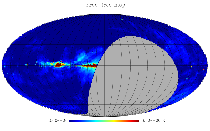
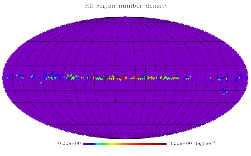
Figure 11: Map of free-free emission at $1.4$ GHz resulting from our procedure (top). Map of Galactic H II region number density taken from the Kuchar & Clarke catalogue (bottom).

Figure 12: Free-free emission at 1.4 GHz along the Galactic plane ($b=0^{\circ}$) as obtained from our procedure (solid). The data are smoothed on $2^{\circ}$ angular scale. The number density of the H II region of the Kuchar & Clarke catalogue is shown for comparison (dashed).

In our free-free map (see Figure 11) the emission is concentrated on the Galactic plane, in particular towards both the Galactic Centre and the area between $75^{\circ}<l<90^{\circ}$. Furthermore, it is very low at mid and high Galactic latitudes. Figure 11 also shows the distribution of the Kuchar & Clarke H II regions: they too are concentrated on the Galactic plane and their number is larger where our map shows the largest and strongest structures. This is also suggested by Figure 12, which compares the free-free emission from our map with the H II region number-density along the Galactic plane. Our map is well traced by the free-free emitting sources, making us confident that we are subtracting thermal contributions properly.

A further test is allowed by the study of thermal emission along the Galactic plane described in RR88.

A relevant contribution (up to $15\%$ at $408$ MHz) is found in the $15^{\circ}<l<50^{\circ}$ area as well as a concentration of H II regions at $l\simeq 75^{\circ}$ in the Cygnus, where a spectral-index flattening reveals the presence of a strong thermal component. These areas correspond to the most evident structures in our map, showing the template is also able to reproduce important free-free diffuse emission sources.

Finally, a comparison of our free-free map at 1.4 GHz with the Reich map at the same frequency shows that in some areas on the Galactic plane the estimated free-free contribution is 50% or more of the total emission. This is an a posteriori confirmation that the free-free contribution in the Haslam and Reich maps is not negligible.

4.3 The Impact of Faraday Rotation

A check of our polarization angle map is performed by comparing Heiles angles with the data of the Parkes Southern Galactic Plane survey at 2.4 GHz (D97).

However, as pointed out in Section 2.4, Parkes data cannot be representative of intrinsic polarization angles because of their high RM values. To account for them we introduce a compensation by using equation (17). As shown by SF83, this behaviour is correct in the Parkes area but in the region around $l\sim 300^{\circ}$, where a strong deviation is observed and a typical value of RM cannot be defined.

The Parkes survey covers the Galactic plane in the $l<6^{\circ}$, $238^{\circ}<l<360^{\circ}$ and $|b|<5^{\circ}$ area with a resolution of $\simeq 10\arcmin$ at $2.4$ GHz.

We smooth both maps on $4^{\circ}$ angular scale to limit the impact of local RM variations. Larger scales cannot be addressed since they are marginally compatible with the $10^{\circ}$ width of the Parkes survey. Furthermore, as already discussed, starlight data are rotated by $90^{\circ}$ to match the synchrotron polarization angles orientation.

Figure 5 shows that Heiles angles vary smoothly with the Galactic longitude. Parkes data are slowly varying as well but in correspondence of extended sources (D97). Here data show peculiar features (discontinuities, inversions, sudden rotations) which even the smoothing procedure is not able to remove, the sources extending over several degrees. These regions are excluded from our comparison since the RM model synthesized by equation (17) just describes the general behaviour of background emission. In details, following the D97 identification we exclude the regions $260^{\circ}<l<272^{\circ}$ (Vela SNR), $272^{\circ}<l<285^{\circ}$ (a bright source with no total intensity counterpart), $320^{\circ}<l<340^{\circ}$ (SNR), $0^{\circ}<l<6^{\circ}$ (Galactic centre with several peculiar structures).

We divide the rest of the Parkes surveys in six patches, of at least $8^{\circ}\times 4^{\circ}$, characterized by a small variation of the polarization-angle pattern.

For each selected patch we average the difference between Parkes and Heiles polarization angles, the latter being rotated by $90^{\circ}$. Should Heiles angles describe the magnetic field responsible for synchrotron emission, these differences would match the polarization angle variations induced by RM. These two quantities are reported in Figure 13, whereas their difference, expected to be zero, is shown in Figure 14.

The general agreement between Parkes-Heiles differences and RM effects confirms that Heiles data provide a reliable template for the polarization angles of Galactic synchrotron emission.

Figure 13: Differences between polarization angles in the Parkes survey and in our template (filled). Faraday rotation values at 2.4 GHz as resulting from equation (17) are shown for comparison (open).

Figure 14: Differences between the two quantities plotted in Figure 13. The dashed line shows the expected value.

Finally, we stress that the evident disagreement at approximatively $l\sim 300^{\circ}$ is not surprising, being RM data in this area not well fitted by equation (17).

Both SF83 and D97 note that this region presents a complex situation where a sudden inversion of polarization angles takes place, probably due to the transition from the Carena to the Centaurus arms ($l\simeq 302^{\circ}$). Here a $180^{\circ}$ rotation of magnetic field occurs generating large changes in RMs.

5 Conclusions

In this paper we have presented a new approach for a template of the polarized Galactic synchrotron emission which, free from Faraday rotation effects, can be better extrapolated to the cosmological-window frequency range (20–100 GHz). Differing from previous spatial models (Giardino et al. 2002, Kogut & Hinshaw 2000), it is intended to provide the real spatial distribution of both polarized intensity and polarizationn angles. We notice that most previous works adopted a complementary approach based on angular frequency rather than real space (Tucci et al. 2000, 2002; Baccigalupi et al. 2001; Giardino et al. 2001; Bruscoli et al. 2002). In fact, angular spectra are commonly used for scale separation in the case of CMB, since they are suitable for cosmological parameters fitting. However, the shape of polarization angular spectra found at frequencies $\sim 1$ GHz, being affected by Faraday rotation, cannot be confidently extrapolated to the cosmological window. This point was raised up by Tucci et al. (2001) and Bruscoli et al. (2002), who noticed different behaviours in $C_{l}^{P}$ and $C_{l}^{I_{p}}$ spectra at all scales in the range $l\simeq 10\div 10^{4}$, suggesting the latter be less affected by Faraday rotation. In particular, the analysis of the ATCA Test Region at 1.4 GHz (Tucci et al. 2002) shows strong changes of slope at small angular scales for $C_{l}^{X}$ with $X=E,B,P$, but not for $C_{l}^{I_{p}},$ and this seems to be the most dramatic effect of Faraday screens. At present, no method is known for correcting such effects directly on angular spectra. The present model is intended to overcome such a problem too: polarization angular spectra in the cosmological window should be computed on the spatial template rather than simply extrapolated from the direct analysis of low-frequency maps.

The model construction consists in three steps:

1)

The synchrotron total intensity $I$ is estimated from the low-frequency radio surveys, cleaned from free-free emission (see Section 2.1 and 2.2).

2)

The polarized intensity $I_{p}$ is estimated from $I$ by assuming that the Galactic polarized synchrotron emission is local because of the existence of a polarization horizon (see Section 2.3).

3)

The polarization angle map is built up from starlight polarization data (see Section 2.4).

Step 3 is of great importance for building a pattern of Stokes parameters. The available RM measurements suggest in fact that the effects of Faraday rotation on polarization angles are still too relevant in the radio-surveys at 2.7 GHz, the highest available frequency, so that the intrinsic position angles cannot be estimated even with RM corrections in large portions of the sky. In our approach we simply overcome the problem using the starlight optical data (Heiles 2000). The local origin of this catalogue ($\sim$87% of the stars within 2 kpc) and its frequency unaffected by Faraday rotation effects make it a reliable template for polarization angle of the Galactic synchrotron. Our analysis shows also that the sampling of the catalogue is compatible with the SPOrt angular resolution in all the sky but in the North Galactic Pole where it is too sparse.

A set of checks provides the consistency of the model with existing data:

• The free-free map obtained with our procedure well traces the HII region distribution from the Kuchar & Clarke (1997) catalogue. This makes us confident about the validity of step 1.

• The estimate provided for the distance of the polarization horizon (3-6 kpc) is in good agreement with the values obtained by observations, and the polarized intensity $I_{p}$ well reproduces the main structures observed in the BS76 data at 1.4 GHz. Both facts support the reliability of steps 1 and 2.

• The slopes of polarized angular power spectra $C_{\ell}^{E}$, $C_{\ell}^{B}$, $C_{\ell}^{P}$ and $C_{\ell}^{I_{p}}$ agree with those measured for large areas of the 1.4 GHz BS76 survey, within the large error bars declared by Bruscoli et al. (2002); discrepancies appear in the comparison with results at frequencies below 800 MHz.

• The polarization angles of the template are in good agreement with those measured at 2.4 GHz (D97) and corrected for Faraday rotation effects in those regions where the D97 position angles show a smooth dependence on coordinates.

The last two items prove the validity of step 3. In this connection, we wish to stress that a perfect agreement is not expected at all for angular power spectra, even in the case of the 1.4 GHz BS76 survey. Since a conspicuous flattenig of polarization power spectra is attributed to Faraday rotation, we expect the power spectra derived from our template to be somewhat steeper than those of Bruscoli et al (2002). This effect is not so clear due to the large error bars and different sky coverages, but perhaps it is already marginally significant. The results in Table 2 can be compared to the weighted averages of the 1.4 GHz angular slopes provided by Bruscoli et al. (2002), namely $\alpha_{E}=1.8\pm 0.3$ and $\alpha_{B}=1.4\pm 0.3.$ We note also that we are unable to find differences between $\alpha_{P}$ and $\alpha_{PI}$ in our template. It is an open question, whether such slopes will be eventually found to be equal in synchrotron spectra for vanishing Faraday effects.

In conclusion, our method results in a template of the polarized Galactic synchrotron emission at 1.4 GHz free from Faraday rotation effects, which can thus be directly extrapolated to the cosmological window frequencies. In this range the Galactic synchrotron emission is expected to play the leading role in the foreground contamination of CMBP data. Following Platania et al. (1998), the extrapolation can be performed using a power law with spectral index $\beta\sim 3.0$. As mentioned in Section 1 this template, together with the simulated CMBP data, provides a more reliable source map to test data processing and foreground separation algorithms for CMBP experiments in the 20-100 GHz range. The model has been developed so far for a FWHM = $7^{\circ}$ angular resolution, matching the needs of large scale CMBP experiments like SPOrt, and allows to build angular spectra only up to $\ell\simeq 20$. At present, the position angle data represent the major constraint, the Heiles data being sampled on a few degree distance. However, we believe that the method can be applied at subdegree scales as well, when a complete set of data on these scales will be available.

Appendix A Distance $L(l,b)$ between the Sun and a Galactic Halo point

The point $P$ on the Galactic halo (radius $R=15$ kpc) at Galactic coordinate ($l$, $b$) is the intersection between the sphere representig the halo and the line starting from the Sun position. In the Sun reference frame (see Figure 15) this intersection can be expressed as:

$$\left\{\begin{array}[]{ccc}(x-d)^{2}+y^{2}+z^{2}&=&R^{2}\\ \\ \displaystyle{\frac{x}{\cos(b)\cos(l)}}&=&\displaystyle{\frac{y}{\cos(b)\sin(l)}}\\ \\ \displaystyle{\frac{x}{\cos(b)\cos(l)}}&=&\displaystyle{\frac{z}{\sin(b)}}\end{array}\right.$$

where $d$ is the Sun distance from the Galactic Centre (GC). The solution of the system provides the $P$ coordinates

$$\left\{\begin{array}[]{lll}x\!\!\!\!&=&\!\!\!\!d\cos^{2}(b)\cos^{2}(l)\left[1\pm\sqrt{1+\left(\displaystyle{\frac{R^{2}/d^{2}-1}{\cos^{2}(b)\cos^{2}(l)}}\right)}\right]\\ y\!\!\!\!&=&\!\!\!\!x\tan(l)\\ \\ z\!\!\!\!&=&\!\!\!\!x\tan(b)/\cos(l)\end{array}\right.$$

Therefore, the distance $L(l,b)$ is given by

$$L(l,b)=d\,\cos(b)\,\cos(l)\,\left[1+\sqrt{1+\frac{(R^{2}/d^{2}-1)}{\cos^{2}(b)\,\cos^{2}(l)}}\right]$$ (28)

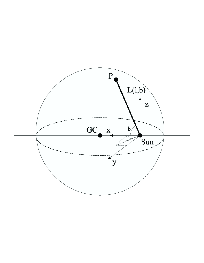
Figure 15: Thickness of synchrotron emitting region $L(l,b)$ along the line of sight ($l$, $b$) for our simple spherical model: it is the distance of the point $P$ on the halo from the Sun.

References

- [1] Baccigalupi C., Burigana C., Perrotta F., De Zotti G., La Porta L., Maino D., Maris M., Paladini R., 2001, A&A, 372, 8
- [2] Brouw W.N., Spoelstra T.A.T. 1976, A&AS, 26, 129 (BS76)
- [3] Brown J.C., Taylor A.R., 2001, AJ, 563, L31 (BT01)
- [4] Bruscoli M., Tucci M., Natale V., Carretti E., Fabbri R., Sarra C., Cortiglioni S., 2002, NewA. 7, 171
- [5] Carretti E. et al., 2002, in S. Cecchini, S. Cortiglioni, R. Sault, C. Sbarra, eds., AIP Conf. Proc. 609, Astrophysical Polarized Backgrounds, New York, p. 109
- [6] Cortiglioni S. et al., 2002 in L.W. Chen, C.P. Ma, K.W. Ng, U.L. Pen, eds., ASP Conf. Ser. 257, AMiBA 2001: High-Z clusters, missing barions, and CMB polarization, p. 243
- [7] de Oliveira - Costa A., Tegmark M., Guti rrez Carlos M., Jones Aled W., Davies R.D., Lasenby A.N., Rebolo R., Watson R.A., ApJ, 527, L9.
- [8] Dodelson S., 1997, ApJ, 482, 577
- [9] Duncan A.R., Haynes R.F., Jones K.L., Stewart R.T., 1997, MNRAS, 291,279 (D97)
- [10] Duncan A.R., Reich P., Reich W., Fürst E., 1999, A&A, 350,447 (D99)
- [11] Fosalba P., Lazarian A., Prunet S., Tauber J.A., 2002, ApJ, 564, 762
- [12] Gaensler B.M., Dickey J.M., McClure-Griffiths N.M., Green A.J., Wieringa M.H., Haynes R.F., 2001, ApJ, 549, 959
- [13] Giardino G., Banday A.J., Bennet K., Fosalba P., Gorski K.M., O’Mullane W., Tauber J., Vuerli C., 2001, in A.J. Banday, S. Zaurobi, M. Bartelmann, eds., Springer-Verlag Series Proc. of the MPA/ESO/MPE Conference, Heidelberg, p. 458
- [14] Giardino G., Banday A.J., Gorsky K.M., Bennet K., Jonas J.L., Tauber J.A., 2002, A&A, 387, 82
- [15] Haslam C.G.T., Stoffel H., Salter C.J., Wilson W.E., 1982, A&AS, 47, 1
- [16] Heiles C., 2000, AJ, 119, 923
- [17] Junkes N., Fürst E., Reich W., 1990, eds, Proc. IAU Symp. 140, Galactic and intergalactic magnetic fields. Kluwer Academic Publishers, Dordrecht, p. 63
- [18] Kamionkowski M., Kosowky A., 1998, PRD, 57, 685
- [19] Kesteven M., 2002, in S. Cecchini, S. Cortiglioni, R. Sault, C. Sbarra, eds., AIP Conf. Proc. 609, Astrophysical Polarized Backgrounds, New York, p. 156
- [20] Kogut A., Banday A.J, Bennett, C.L., Górski K.M., Hinshaw G., Smooth G.F., Wright E.L., 1996, ApJ, 464, L5
- [21] Kogut A., Hinshaw G., 2000, ApJ, 543, 530
- [22] Kovac J., Leitch E.M., Pryke C., Carlstrom J. E., Halverson N. W., Holzapfel W. L., 2002, preprint astro-ph/0209478
- [23] Kuchar T., Clark F.O., 1997, ApJ, 488, 224
- [24] Landecker T.L., Uyaniker B., Kothes R., 2002, in S. Cecchini, S. Cortiglioni, R. Sault, C. Sbarra, eds., AIP Conf. Proc. 609, Astrophysical Polarized Backgrounds, New York, p. 9
- [25] Lazarian A., Prunet S., 2002, in S. Cecchini, S. Cortiglioni, R. Sault, C. Sbarra, eds., AIP Conf. Proc. 609, Astrophysical Polarized Backgrounds, New York, p. 32
- [26] Masi S. et al., 2002 in S. Cecchini, S. Cortiglioni, R. Sault, C. Sbarra, eds., AIP Conf. Proc. 609, Astrophysical Polarized Backgrounds, New York, p. 122
- [27] Platania P., Bensadoun M., Bersanelli M., De Amici G., Kogut A., Levin S., Maino D., Smooth G.F., 1998, ApJ, 505, 473
- [28] Prunet S., Sethi S.K., Bouchet F.R., Miville-Deschenes M.-A., 1998, 339, 187
- [29] Reich P., Reich W., 1988, A&AS, 74, 7
- [30] Reich W., A&A Suppl. Series, 1982, 48, 219
- [31] Revenu B., Kim A., Ansari R., Couchot F., Delabrouille J., Kaplan J., A&AS, 1982, 142, 499
- [32] Reynolds R.J., Haffner L.M., 2000, IAU Symposium N. 201 ASP conf. Proc. Ser. in press
- [33] Sazhin M.V., Benitez N., Astrophys. Lett. Commun., 1995, 32, 105
- [34] Sbarra C., Carretti E., Cortiglioni S., Zannoni M., Fabbri R., Macculi C., Tucci M., 2003, submitted to A&A
- [35] Simard-Normandin M. & Kronberg P.P., 1980, ApJ, 242, 74
- [36] Sofue Y., Fujimoto M., 1983, AJ, 265, 722 SF83
- [37] Tegmark M., Eisenstein D.J., Hu W., de Oliveira-Costa A., 2000, ApJ, 530, 133
- [38] Tucci M., Carretti E., Cecchini S., Fabbri R., Orsini M., Pierpaoli E., 2000, NewA, 5, 181
- [39] Tucci M., Carretti E., Cecchini S., Nicastro L., Fabbri R., Gaensler B.M., Dickey J.M., McClure-Griffiths N.M., 2002, in S. Cecchini, S. Cortiglioni, R. Sault, C. Sbarra, eds., AIP Conf. Proc. 609, Astrophysical Polarized Backgrounds, New York, p. 60
- [40] M. Tucci, E. Carretti, S. Cecchini, L. Nicastro, R. Fabbri, B.M. Gaensler, J.M. Dickey, N.M. McClure-Griffiths, 2002, ApJ 579, 607
- [41] Uyaniker B., Fürst E., Reich W., Reich P., Wielebinski R., 1999, A&AS, 138, 31
- [42] Zaldarriaga M., 1998, PhD Thesis, M.I.T.
- [43] Zaldarriaga M., Spergel D. N., Seljak U., 1997, ApJ, 488, 1
- [44] Zannoni M. et al., 2002, in S. Cecchini, S. Cortiglioni, R. Sault, C. Sbarra, eds., AIP Conf. Proc. 609, Astrophysical Polarized Backgrounds, New York, p. 115