A robust algorithm for sky background computation in CCD images

In this paper we present a non-interactive algorithm to estimate a representative value for the sky background on CCD images. The method we have devised uses the mode as a robust estimator of the background brightness in sub-windows distributed across the input frame. The presence of contaminating objects is detected through the study of the local intensity distribution function and the perturbed areas are rejected using a statistical criterion which was derived from numerical simulations. The technique has been extensively tested on a large amount of images and it is suitable for fully automatic processing of large data volumes. The implementation we discuss here has been optimized for the ESO-FORS1 instrument, but it can be easily generalized to all CCD imagers with a sufficiently large field of view. The algorithm has been successfully used for the $UBVRI$ ESO-Paranal night sky brightness survey (Patat patat (2003)).

1 Introduction

The study of the night sky brightness is fundamental to monitor the quality of very dark astronomical sites and sets the stage for the study of a whole series of effects which take place in the upper layers of Earth’s atmosphere (Leinert et al. leinert98 (1998) and references therein).

With the exception of a very few cases, all night sky brightness surveys are executed with photoelectric devices coupled to small telescopes and usually span a limited number of nights (Benn & Ellison benn (1998)), distributed across several years. For these reasons, the data are usually rather scanty and suffer from the inclusion of bright stars ($V\geq$13; see for example Walker walker88 (1988)).

Nowadays, with the availability of large telescopes equipped with CCD imagers and the possibility of reducing the data via dedicated pipelines, the paradigm is changing and different approaches become feasible.

In this spirit, during the beginning of year 2000 we have started a project to monitor the $UBVRI$ night sky brightness at ESO-Paranal Observatory (Chile) as part of the quality control (QC) procedures implemented for the FOcal Reducer/low dispersion Spectrograph (hereafter FORS1). This multi-mode optical instrument, which is mounted at the Cassegrain focus of ESO-Antu/Melipal 8.2m telescopes (Szeifert szeifert (2002)), has two remotely exchangeable collimators, which give an imaging field of view of 6′. 8$\times$6′. 8 (standard resolution, SR) and 3′. 4$\times$3′. 4 (high resolution, HR) respectively.

FORS1 is offered during dark time both in Visitor Mode (VM) and Service Mode (SM). Imaging data obtained during SM runs are bias and flat-field corrected by the pipeline and undergo a series of quality checks before they are finally distributed to the users. Due to the high number of imaging frames produced by this instrument (more than 4500 from April 2000 to September 2001) and the variety of scientific cases which drive it, it is clear that a complete and systematic study of the night sky brightness can be performed only by means of a robust and automatic procedure, capable of identifying and rejecting all the cases which are not suitable for sky background measurements (e.g. large galaxies, crowded stellar fields and so on).

In this work we present and discuss the algorithm we have specifically designed for this purpose, while the results of the night sky brightness survey are reported in Patat (patat (2003)).

The paper is organized as follows. In Sec. 2 we discuss the problems connected with the sky background measurement in digital images, while Sec. 3 deals with the technique we have adopted to compute the mode of the image intensity distribution. The algorithm we have devised to identify the presence of contaminating objects in the field and the tests we have performed on real FORS1 data are presented in Sec. 4 and 5 respectively. Finally, in Sec. 6 we summarize our conclusions.

2 Problems in estimating the sky background

Widely available programs for object detection and photometry like DAOPHOT (Stetson 1987) and Sextractor (Bertin & Arnouts 1996) use the mode of the image intensity distribution to estimate the local background or to construct the background map of a two-dimensional frame. In fact, besides its robustness, the mode is a statistically powerful estimator, being the most probable value of the background brightness in a given region of the image.

The use of the mode as the maximum-likelihood estimator for the sky background implicitly assumes that the image has some regions which are not seriously contaminated by any astronomical object. Of course distant and faint galaxies (and stars) will always be present, but we will consider them as part of the global background throughout this paper. Therefore, when we talk about contaminating objects, we mean objects which are detectable in the image, well above the background noise. There is also another assumption that one has to make, i.e. that it is really improbable that the images to be analysed are filled by a single extended object with a roughly constant surface brightness. In fact this is the only case where one would have an overall background increase without having any secondary effects on the intensity distribution function and in that case the process would lead to an overestimate of the sky background. In the case of FORS1 frames, especially with the commonly used SR collimator field of 6′. 8$\times$6′. 8, this assumption seems reasonable.

Due to the field of view of FORS1 and the wide variety of scientific projects which are carried out by this multi-mode instrument, one expects to deal with very different astronomical objects, which would perturb in a different way the local sky background. Possible examples are comets, clusters of galaxies, outskirts of big spirals, large ellipticals, diffuse nebulosities, crowded stellar fields and so on. In all these cases there still might exist parts of the image which are suitable for a sky background measurement. For this reason it is clear that the analysis has to be performed using sub-windows distributed on a grid across the input image. The choice of the sub-window size has to be done in such a way that this is neither too small, because in that case the fraction of uncontaminated pixels might become statistically insignificant, nor too big, otherwise the probability of including large diffuse objects becomes large. After running some tests we have seen that a 300$\times$300 px sub-window (which corresponds to 1 arcmin² for the SR collimator) gives satisfactory results. Since the guide probe of FORS1 is sometimes vignetting the outer parts of the images, we have decided to use the central 1800$\times$1800 px region of the detector only. This allows one to analyse the images in a 6$\times$6 sub-windows grid including 9$\times$10⁴ px each.

Of course there is always the possibility that none of the sub-windows is clean enough to allow for a reliable measurement. A few examples are galactic stellar fields with heavily saturated stars, outer parts of globular clusters, nearby interacting galaxies and close-by comets, just to cite a few real examples we encountered during this analysis.

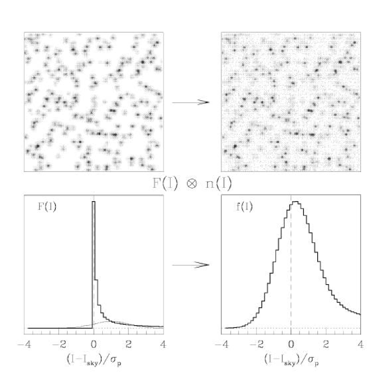
Figure 1: Illustration of the effect on the intensity distribution when a Poissonian noise is added to a stellar field with a constant background $I_{sky}$. The vertical scale in the lower plots is arbitrary, while the intensity $I$ is counted from the input $I_{sky}$ value and normalised to $\sigma_{p}=\sqrt{I_{sky}}$. The solid thin curve in the lower left plot depicts the contribution to the final intensity distribution by the value of $F(I)$ at $I=I_{sky}+\sigma_{p}$.

The difficulties one faces in estimating the background are easily understood from the following considerations. If the images to be analysed were noiseless and the sky background constant and equal to $I_{sky}$, the solution of the problem would be trivial. In fact, in this case, the corresponding intensity distribution function $F(I)$ would be 0 for $I<I_{sky}$, would then suddenly peak at $I=I_{sky}$ and finally show an extended tail, whose shape depends on the number and intensity of contaminating objects. This is illustrated in the left part of Fig. 1, where we have presented an artificial stellar field and its intensity distribution. As usual, Nature behaves in a more subtle way and due to the photon statistics (and marginally to detector read-out) the images we are going to deal with are always affected by noise. From a mathematical point of view it is very easy to predict the noise effect on the intensity distribution. In fact, if $n(I)$ is the noise distribution, the observed intensity distribution is simply given by:

$$f(I)=\int_{-\infty}^{I}F(I-z)\;n(I,z)\;dz$$ (1)

i.e. the convolution $F\otimes n$ of the signal $F(I)$ with a variable response function $n(I,z)$, which can be expressed as $n(I,z)=1/\sqrt{2\pi\;z}\;\;exp[-\frac{1}{2}(z^{2}/(I-z)]$, provided that the read-out noise is negligible. From these simple considerations it is clear that what really matters for the degradation of the resulting peak sharpness and the consequent uncertainty in the estimate of its original position is the shape of the input distribution function $F(I)$ within $\sim$5$\sqrt{I_{sky}}$ from its peak, while the behaviour at higher intensities is unrelevant (see Fig. 1, right plots). With respect to these effects, it is quite instructive to look at the results of some numerical simulations. In Fig. 2 we have plotted the relative intensity distributions of three 300$\times$300 px artificial frames with a fixed value of the sky background ($I_{sky}$=5000 electrons) on which we have randomly injected 10, 200 and 500 stars respectively. We have used a Moffat profile for the stars with $\beta$=4 and a FWHM of 5.3 px. In the case of FORS1 and SR collimator this would correspond to a field of 1 arcmin² and a seeing of 1^′′. The peak intensity of the stars was randomly generated in the range 0-10⁴ electrons.

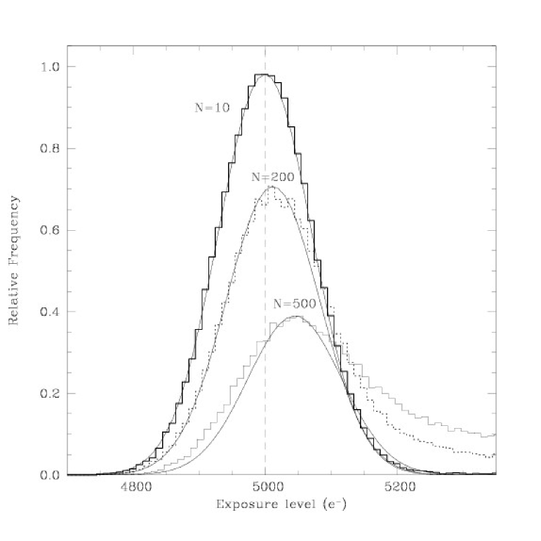
Figure 2: Intensity distributions for three simulated images obtained injecting 10, 200 and 500 stars (from top to bottom) on a background $I_{sky}$=5000 e^- with a Poissonian noise distribution. The solid curves are Gaussian profiles centred on the distribution mode and having the $\sigma$ expected for a Poissonian noise (see text for more details).

Basically three effects are visible as the number of stars grows: A) the mode $\langle I\rangle$ of the distribution steadily increases; B) the distribution core width increases; C) the distribution becomes more and more skewed, with a tail appearing at the highest intensities. Clearly effect A and B will respectively lead to overestimates of the sky background $I_{sky}$ and the noise, which in the case of an uncontaminated field is expected to be $\sigma_{p}=\sqrt{I_{sky}}$, according to the Poissonian statistics. One possible solution to this problem is achieved by reconstructing the intensity distribution one would have if no contamination effects were present. A good example of such a solution is represented by the asymmetric clipping algorithm developed by Ratnatunga & Newell (ratna (1984)), which computes the background distribution via an iterative clipping of the right wing of the perturbed intensity distribution.

Due to the high number of available FORS1 frames and the purpose of this work, we can afford a different approach. Instead of attempting to reconstruct the underlying sky background intensity distribution in contaminated regions, we rather try to identify these regions and exclude them from all further calculations. For this purpose we have devised a simple and robust test that can be used to estimate the degree of contamination in an image and operated in an automatic way on large amounts of data.

The first step in the application of our method is the mode estimate, which we describe in the next section.

3 Mode estimate

The mode $\langle I\rangle$ of a distribution $f(I)$ is defined as the most probable value of $I$ (see for example Lupton 1993) or, in other words, the value of $I$ where $f(I)$ takes its maximum value. For moderately skewed distributions the mode can be approximately computed as $\langle I\rangle\simeq 3\times median-2\times mean$ (Kendall & Stuart 1997). Unfortunately, the observed intensity distributions in FORS1 images often show very extended tails, due to several effects like saturated stars, cosmic-ray events and so on. While this tail usually does not affect the mode, it does perturb the mean and the above formula would lead to wrong results. A possible solution is given by the application of this approximation after an iterative clipping of the distribution around its median, as it is done for example in Sextractor (Bertin & Arnouts 1996). In practice one is forced to use this method when one has to compute the background map of an image using small sub-windows. In fact in that case the statistics would be too poor to compute the mode in a reliable way directly using the distribution shape.

This is not the case here, since we are more interested in an average value rather than in a map of the background within the same image. For this reason we can perform our analysis in much larger sub-windows so that we can build up a very good signal-to-noise distribution function. This allows us to compute the mode just using its definition, without any loss of generality and in a very robust way.

3.1 Introducing the Optimal Binning Technique (OBT)

Since we are dealing with discrete distribution functions, finding the mode implies that the data have to be binned and the maximum of the distribution has to be found. To reduce the noise due to the finite (and possibly large) bin size $\Delta I$, we have chosen to refine the direct mode estimate using a quadratic interpolation on the modal bin and the two adjacent bins (see for instance Spiegel 1988). If $I_{m}$ and $f_{m}=f(I_{m})$ are the values of the intensity and intensity distribution in the modal bin and $(I_{r},f_{r})$,$(I_{l},f_{l})$ are the corresponding values in the two adjacent bins respectively, then the mode $\langle I\rangle$ is estimated as the value of $I$ where the interpolating parabola reaches its maximum. One can show that this is given by the following expression:

$$\langle I\rangle=I_{m}+\frac{f_{l}-f_{r}}{f_{l}-2f_{m}+f_{r}}\;\frac{\Delta I}{2}$$ (2)

This correction has the effect of moving the estimated mode $\langle I\rangle$ within the whole bin $\Delta I$ according to the local shape of the distribution function. The modal bin boundaries are reached when $f_{m}=f_{l}$ or $f_{m}=f_{r}$ (provided that $f_{l}\neq f_{r}$). Numerical simulations have shown that the parabolic interpolation is very effective in reducing the error on the mode estimate (see below), at least for the kind of distributions considered here. For more general cases, the interpolation option will improve the mode accuracy only if the asymmetry of the distribution around the mode perturbs $(f_{l}-f_{r})$ significantly less than the average value of the correction corresponding to an offset of the central bin.

The choice of bin size is critical. If the bin $\Delta I$ is too small the resulting histogram will be too noisy to give a robust estimate of $\langle I\rangle$. On the other hand, if $\Delta I$ is too large, then the mode estimate will be affected by a large uncertainty due to the small signal-to-noise in the two outer bins. For this reason we need to find an optimal value for $\Delta I$ which minimises the error on the mode.

For this purpose we have run a series of numerical simulations of uncontaminated windows with a known sky level on top of which we have added a Poissonian noise and a typical read-out noise (6 electrons). For each of the simulated frames the mode was estimated using the parabolic interpolation described above. This has been done for different values of the bin size $\Delta I$ and the number of pixels $N=n_{pix}^{2}$ included in each testing window. For each pair ($\Delta I$,$n_{pix}$) we have performed 5000 simulations. What one sees is that for a given value of $n_{pix}$, the RMS deviation of the estimated mode from the known input value $I_{sky}$ decreases as $\Delta I$ increases, reaches a minimum and then grows again, as expected from the above considerations (see also Fig. 4). For this reason it makes sense to adopt the value of $\Delta I$ where the RMS error $\epsilon_{RMS}$ reaches its minimum as the optimum bin size for the mode estimate.

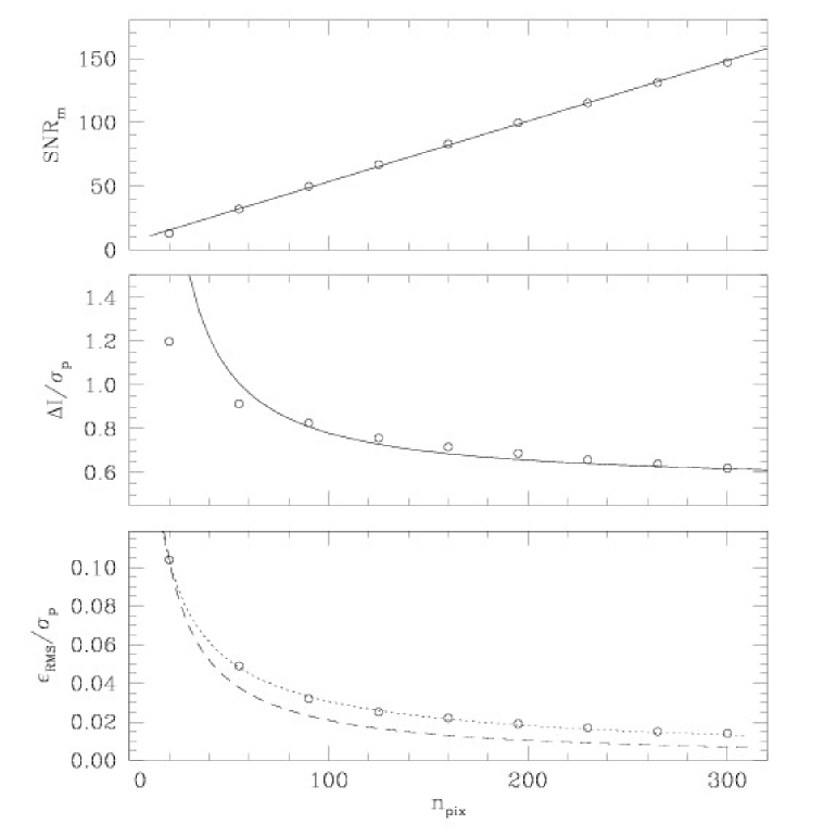
Figure 3: Upper panel: Signal-to-noise ratio $SNR_{m}$ reached in the modal bin for the optimal value of $\Delta I$ as a function of $n_{pix}$. The solid line represents a linear fit to the data with $n_{pix}\geq$90. Middle panel: normalised optimal bin width. The solid line traces Eq. 8. Lower panel: optimal values of the RMS error on the mode. The dotted line is a best fit to the data ($\epsilon_{RMS}\propto n_{pix}^{-0.75}$) while the dashed line traces the law $\epsilon_{RMS}\propto n_{pix}^{-1}$. In all panels each point is the result of 5000 simulations.

Before we proceed with the presentation of the results, we want to discuss a few more points. The pixel counts in the intensity distribution bins obey Poissonian statistics. This implies that if $f(I)$ is the number of pixels falling in a given bin, the RMS uncertainty on $f(I)$ is simply given by $\sqrt{f(I)}$ and hence we can define a signal-to-noise ratio $SNR=\sqrt{f(I)}$. In particular, we can introduce $SNR_{m}$, i.e. the signal-to-noise ratio reached in the modal bin. If $f$ is the fraction of pixels falling in the modal bin, we have obviously

$$f=(SNR_{m}/n_{pix})^{2}$$ (3)

Having this in mind, we can now have a look at the behaviour of $SNR_{m}$ as a function of $n_{pix}$ when the optimal bin size is used to estimate the mode in our simulations. This is portrayed in the upper panel of Fig. 3, where one can easily see that $SNR_{m}$ depends almost linearly on $n_{pix}$. In the range $90\leq n_{pix}\leq 300$, the best fit to the simulated data (see Fig. 3, upper panel) gives

$$SNR_{m}\simeq 6.2+0.48\;n_{pix}$$ (4)

For large values of $n_{pix}$ this relation can be approximated as $SNR_{m}\approx n_{pix}/2$, which means that optimal results are obtained when $\sim$25% of the pixels fall in the modal bin.

Having this result, it is easy to compute the optimal fraction $f$ of pixels by means of Eq. 3 and Eq. 4 (or its approximate expression). Then, assuming the underlying distribution $f(I)$ to be a Gaussian with $\sigma=\sigma_{p}$, one can derive the corresponding bin size in terms of $\sigma_{p}$ as

$$\Delta I=2\;k(f)\;\sigma_{p}$$ (5)

where $k$ is implicitly defined by the following equation:

$$f=\frac{1}{\sqrt{2\pi}\sigma_{p}}\int_{\langle I\rangle-k\sigma_{p}}^{\langle I\rangle+k\sigma_{p}}\exp\left[{-\frac{(I-\langle I\rangle)^{2}}{2\sigma_{p}^{2}}}\right]\;dI$$ (6)

This equation can be solved numerically and the solution fitted by a low order polynomial. For $f\leq$0.33 ($n_{pix}>$60), the solution can be approximated rather accurately by the following expression:

$$k(f)\simeq 1.28\;f$$ (7)

Finally, using Eqs. 5 and 7 one can easily compute the optimal bin width. For $n_{pix}\geq 90$ we can approximate the expression for the optimal bin as follows:

$$\frac{\Delta I}{\sigma_{p}}\simeq 2.6\;\left(0.48+\frac{6.2}{n_{pix}}\right)^{2}$$ (8)

while, for very large values of $n_{pix}$, the ratio between the optimal bin size $\Delta I$ and $\sigma_{p}$ approaches asymptotically the value 0.6. The result is shown in the central panel of Fig. 3, where we have normalised the optimal bin to $\sigma_{p}$ to remove the dependency on the sky level. The comparison between the predicted values (solid line) and the results of the simulations are in good agreement across all the $n_{pix}$ explored range.

Finally, the RMS deviation from the input value in our simulations clearly decreases for increasing values of $n_{pix}$, as shown in the lower panel of Fig. 3. For comparison we have overplotted the $n_{pix}^{-1}$ law (dashed line) expected if the error would scale proportionally to the overall signal-to-noise ratio. It is interesting to note that the RMS error in the simulations decreases at a slower rate, approximately as $n_{pix}^{-0.75}$ (dotted line). We will come back to this point in the next section, when discussing the efficiency of the method in reducing the error; for the time being, we only notice that with $n_{pix}$=20 the expected RMS error for $I_{sky}$=100 electrons is about 1%, which reduces to 0.2% for $n_{pix}$=300.

3.2 Application of OBT to the real case

As we have discussed in Sec. 2, the real data show a variety of contaminating effects, which tend to skew the intensity distribution and affect in different ways the mode estimate. In that section we have also mentioned that the optimal window size for the mode estimate is $n_{pix}$=300. Both simulations and tests with real data show that with such a number of pixels we can achieve RMS errors on the mode smaller than 1% for $I_{sky}\geq$100 electrons, which we believe is a sufficient accuracy for our purposes. For this reason, from now on we will concentrate on the specific case of $n_{pix}$=300 and discuss several aspects of the method application.

In the previous section we have seen that, for a sufficiently large value of $n_{pix}$, the optimal bin size can be expressed as:

$$\Delta I=2.6\;\frac{SNR^{2}_{m}}{N}\;\sqrt{I_{sky}}$$ (9)

Of course this requires to know the value of $I_{sky}$, or at least to have a rough estimate of it. For this purpose, one can approximate it with the median of the distribution $I_{med}$, and $SNR_{m}$ can be computed using Eq. 4. For $n_{pix}$=300 we have $SNR_{m}\simeq$150.

Once this guess value for the bin is computed, the histogram of the intensity distribution between $I_{min}$ and $I_{max}$ is built and the mode is found. Since in the case of skewed distributions the median is only a rough approximation of the mode and the distribution is definitely not Gaussian, the actual signal-to-noise ratio $SNR^{\prime}_{m}$ in the modal bin is measured and from this value a new bin is recomputed as $\Delta I^{\prime}=\Delta I\;(SNR_{m}/SNR^{\prime}_{m})^{2}$. The histogram is recalculated and a new mode value is estimated. This procedure has a clear effect: if the distribution is skewed (and hence less peaked), then a larger bin size is required to achieve the same $SNR_{m}$.

The method has been tested using numerical simulations of uncontaminated 300$\times$300 px windows with a known sky level $I_{sky}$ on top of which we have added a Poissonian noise and a typical read-out noise (6 electrons). For each simulated field, we have then computed the mode $\langle I\rangle$ and the deviation from the input sky background value defined as

$$\epsilon=\frac{\langle I\rangle-I_{sky}}{I_{sky}}$$ (10)

In Fig. 4 we present the results we have obtained for a very low sky background (100 electrons). The RMS deviation $\epsilon_{RMS}$ (solid line) reaches its minimum value (0.2%) for $SNR_{m}$=150, as expected, and so does the maximum error $\epsilon_{max}$ (dotted line). In the same figure we have also plotted the RMS error one obtains without using the refinement given by Eq. 2 ($\epsilon^{\prime}_{RMS}$, dashed line). This shows that the two methods give optimal results at two different bin sizes. In such conditions the interpolation reduces the RMS error by about a factor of 6. For comparison we have also plotted the bin half width (long-dashed line), which can be assumed as an estimator of the maximum deviation when the parabolic interpolation is not used.

On the basis of these results one would tend to adopt $SNR_{m}$=150, but there is a caveat that we have to keep in mind. These results are valid for uncontaminated distributions, where the signal-to-noise ratio $SNR_{m}$ in the modal bin is reached using the bin size given by Eq. 9. Since real distributions are contaminated, a larger bin size is required in order to achieve the same $SNR_{m}$ and this in turn generates larger errors. The simulations and extensive tests with real data have shown that a good compromise is reached using $SNR_{m}$=120 which, for mildly contaminated distributions gives maximum errors smaller than 1% for a background level of 100 electrons (see Tab. 1).

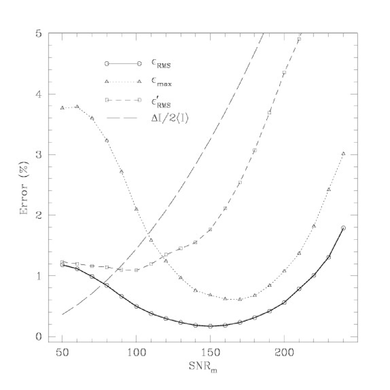
Figure 4: Estimated RMS mode errors (solid line) from simulated 300$\times$300 px un-contaminated windows as a function of $SNR_{m}$. The maximum error is traced with a dotted line, while the dashed line indicates the RMS error when the parabolic interpolation is not used. Finally, the long-dashed line indicates the percentage bin half width. The values for each $SNR_{m}$ level are the result of 5000 simulations.

To see how the error behaves as a function of the sky background, we have performed another set of similar simulations, where we have adopted $SNR_{m}$=120 and we have varied the input sky level from 10² to 10⁴ electrons. A total of 5000 simulations per level were executed. The results are presented in Fig. 5 and summarized in Tab. 1.

Table 1: Estimated errors from numerical simulations of 300$\times$300 px uncontaminated windows for three different values of the sky background. Maximum errors are indicated within parenthesis. A total of 5000 simulations per sky level and $SNR_{m}$ value were performed.

$SNR_{m}$	f (%)	$n_{b}(\pm\sigma)$	$\Delta I$/$\langle I\rangle$(%)				RMS error (%)
			$10^{2}$	$10^{3}$	$10^{4}$		$10^{2}$	$10^{3}$	$10^{4}$
120	16.0	5	4.7	1.3	0.4		0.25 (1.00)	0.07 (0.27)	0.02 (0.11)
150	25.0	3	7.5	2.1	0.7		0.17 (0.60)	0.04 (0.16)	0.02 (0.06)

In the upper panel of Fig. 5 we have plotted the percentage errors $\epsilon$ as a function of the background level. As expected, the percentage RMS error, traced with a solid line, decreases for increasing values of $\langle I\rangle$, following very well the usual law for the standard error of the average:

$$\sigma_{\langle I\rangle}=\sqrt{\frac{\langle I\rangle}{N_{eff}}}$$ (11)

with the difference that $N_{eff}$ is smaller than the total number $N$ of pixels. For this reason, $N_{eff}$ can be considered as the effective number of data points drawn from the original set one would have to use to get the same RMS error when adopting the average as background estimator. As we have seen at the end of Sec. 3.1, the RMS error scales as $n_{pix}^{-0.75}$, and hence we have $N_{eff}=N^{0.75}$ when the optimal $SNR_{m}$ is adopted. Since we have chosen to use $SNR_{m}$=120, we expect $N_{eff}$ to be even smaller. In fact, fitting Eq. 11 to the simulated data, we get $N_{eff}\sim 1970$. Combining Eq. 9 and Eq. 11 one gets the following relation between the bin size $\Delta I$ and the expected RMS error $\sigma_{\langle I\rangle}$ on the mode:

$$\sigma_{\langle I\rangle}=\frac{N}{\sqrt{N_{eff}}}\;\frac{\Delta I}{2.6\;SNR_{m}^{2}}$$ (12)

Substituting the proper values in this expression, we obtain simply $\sigma_{\langle I\rangle}\simeq 0.05\;\Delta I$, which means that for $SNR_{m}$=120 and moderately contaminated distributions, the expected RMS error on the mode is of the order of 5% of the bin size. This is clearly shown in the lower panel of Fig. 5, where we have plotted the measured error as a function of the relative bin size derived from the same set of simulations previously described. The match between the expected RMS (dotted line) and the observed RMS (dashed line) is fairly good.

In both panels of Fig. 5 we have plotted the maximum errors encountered during the simulations. As one can see, they are well confined within the 5$\sigma$ level (dashed line), which was computed using the RMS error given by the simulations. More precisely, maximum errors lie with a good approximation on the 4$\sigma$ level. From Fig. 5 we can conclude that the expected RMS errors on the mode estimate are below 0.3% at all sky background levels larger than 100 electrons, while maximum errors are always smaller than 1%.

The introduction of artificial stars has the effect of systematically increasing the mode of the distribution with respect to the real value of the sky background (see Sec. 2). For this reason, in the general case of contaminated distributions, we can talk about two different errors. While the former is a random measurement error intrinsic to the adopted method and to the quality of the data, the latter is a systematic error which depends on the intensity distribution of the contaminating objects. As we have said in Sec. 2, we want to use only the cases where the systematic error is smaller than some threshold value. The approach to this problem is described in Sec. 5, while here we focus only on the random errors related to the way the mode is estimated.

To evaluate the effect of contamination on the method error, we have performed several sets of simulations injecting a fixed number of stars $N_{*}$ with random positions on a sky background of intensity $I_{sky}$. The stars intensities $I_{*}$ were uniformly generated in the range $0<I_{*}\leq(I_{sat}-I_{sky})$, where $I_{sat}$ is the detector’s numerical saturation level ($I_{sat}\sim$ 106,000 electrons for the FORS1 detector, high gain). Finally, a Poissonian noise was added to the artificial 300$\times$300 px frames to simulate the photon shot noise and the mode was measured with the OBT using $SNR_{m}$=120. Numerical tests using a more realistic intensity distribution, drawn from observed star counts, show that very similar contamination effects are achieved. The only difference is that one needs to generate much more artificial stars in the non-uniform case, and this makes it numerically less efficient.

As expected, the simulations show that the systematic error grows with $N_{*}$, while the random error keeps obeying to Eq. 12 with a good approximation, at least for $N_{*}<$200 and $\langle I\rangle\geq$ 500 electrons. More precisely, in the case of $N_{*}=200$, the simulations give $\sigma_{\langle I\rangle}\simeq 0.08\;\Delta I$ in the range 10${}^{2}\leq\langle I\rangle\leq$ 10⁴ electrons. We can safely conclude that the RMS errors introduced by the mode determination method we have described in this section are smaller than 0.3% for $\langle I\rangle\geq$ 5$\times$10²-10⁴ electrons. Finally, the RMS error can be conservatively assumed to be 8% of the bin size $\Delta I$ in the same intensity range, which corresponds to $N_{eff}\sim$1000. These values have been used in the remaining sections of this work and for all sky brightness measurements discussed in Patat (patat (2003)).

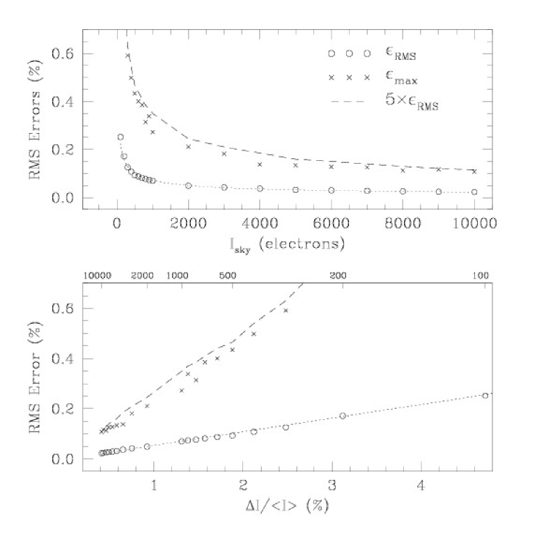
Figure 5: Relative errors on the mode estimate as a function of the sky background (upper panel) and the relative bin size (lower panel). The circles represent the measured RMS deviations, while the dotted line indicates the expected RMS (see Eq. 12). In both panels, the crosses indicate the maximum deviation encountered during the simulations, while the dashed line traces the 5$\sigma$ level. Simulations were performed using $SNR_{m}$=120 and RON=6 electrons.

4 The $\Delta$-test

Once the mode $\langle I\rangle$ of the sky background distribution and the corresponding error $\sigma_{\langle I\rangle}$ have been computed, one is left with the task of recognizing and rejecting contaminated sub-windows, which is the topic of this section.

As we have already mentioned, in an uncontaminated image the intensity distribution $f(I)$ obeys the photon shot noise distribution and hence the expected RMS noise is given by $\sigma_{p}=\sqrt{\langle I\rangle}$. Since the left wing of $f(I)$ is much less disturbed than the right wing (cfr. Fig. 2), we can estimate the underlying background noise using only the $N_{l}$ pixels for which $I\leq$ $\langle I\rangle$. As a robust estimator we have chosen to use the Median Absolute Deviation ($MAD$) from the mode $\langle I\rangle$ applied to the left wing of the distribution:

$$MAD_{l}=median\{\mid I-\langle I\rangle\mid I\leq\langle I\rangle\}$$ (13)

We note that the use of the standard deviation instead of MAD has the effect of over-estimating the noise in the real cases. In fact, the lower tail of the intensity distribution is always affected by defects like bad pixels and possible vignetting. While this fact has a rather strong influence on the standard deviation, it leaves the MAD unperturbed, which is much less sensitive to the presence of outliers.

One can easily show that for a Gaussian distribution the ratio between the standard deviation and the $MAD$ is $\sim$1.483 (Huber 1981). Hence, to have an estimator which has the same meaning of the standard deviation in the normal case, we define $\sigma_{l}=1.483\;MAD_{l}$. This allows one to compare directly $\sigma_{p}$ and $\sigma_{l}$ which, for an uncontaminated distribution, should be approximately the same. To quantify possible deviations from the Poissonian behaviour, we introduce the parameter $\Delta$:

$$\Delta=\frac{\sqrt{\sigma_{l}^{2}-RON^{2}}-\sigma_{p}}{\sigma_{p}}$$ (14)

which equals 0 in the Poissonian case, whilst it gets larger and larger as the deviation from the Poissonian distribution grows. The idea is to try to estimate the unknown systematic error from $\Delta$, which is a measurable parameter. To illustrate this concept we use a real example, where we have performed the analysis on a 300$\times$300 px sub-window centred on the outer parts of the large spiral galaxy NGC 3521, as shown in Fig. 6. The corresponding intensity distribution is shown in Fig. 7, where the mode (indicated by the vertical dashed line) was computed with the Optimal Binning Technique (OBT) we have described in Sec. 3.

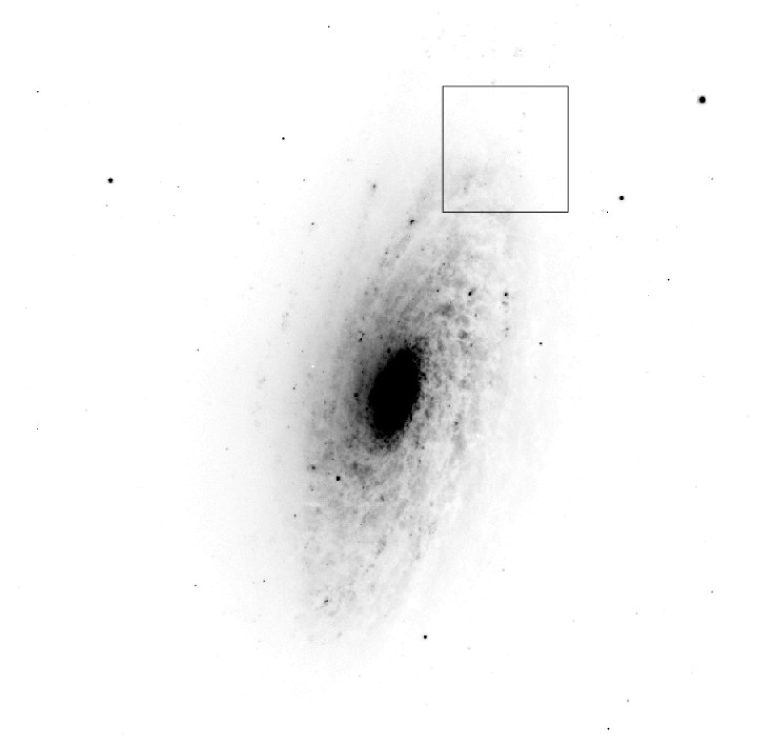
Figure 6: An image of NGC 3521 obtained by FORS1 on 04-04-2000 (R, 30 seconds, standard resolution collimator). The box indicates the test sub-window used for the example described in the text. It includes 300 $\times$ 300 pixels, which correspond to 1^′$\times$1^′ on the sky.

A superficial inspection of the input image shows already that this sub-window is strongly contaminated by diffuse emission from the galaxy’s spiral arms. The mode of the intensity distribution is in fact $\sim$34% higher than the background level manually measured on an object-free area of the same image close to the upper left corner. However, the presence of strong fluctuations within the sub-windows produces a significant increase in the distribution core width, which becomes $\sim$80% larger than the expected photon shot noise ($\Delta$=0.78). This suggests that $\Delta$ may provide a tool to estimate the systematic error induced by contaminating sources and this, coupled with some threshold criterion, would allow us to recognise and disregard the critical cases. To study this possibility, we have executed a series of simulations of contaminated distributions of the same type of those described in Sec. 3.2 for several values of the input sky background intensity $I_{sky}$. For each simulation one can then compute the error $\epsilon$ of the mode estimate (see Eq. 10) and measure $\Delta$. The resulting range in the $\Delta$ parameter can be binned to some suitable value and the corresponding average error $\langle\epsilon\rangle$ computed. In Fig. 8 we have plotted the results one obtains for three different values of the sky background, i.e. 10², 10³ and 10⁴ electrons. The circles represent $\langle\epsilon\rangle$, while the dashed and dotted lines indicate two different estimates of the random error $\sigma_{\langle I\rangle}$; one is the RMS deviation directly computed from the simulated data and the other is estimated using Eq. 11. While the systematic error is clearly due to the presence of contaminating objects, the random error $\sigma_{\langle I\rangle}$ is related to the accuracy of the method one adopts to estimate the mode $\langle I\rangle$ (see Sec. 3).

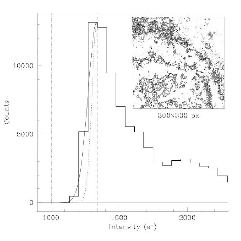
Figure 7: Intensity distribution for the sub-window placed on a outer region of NGC 3521 (see Fig. 6). The vertical lines are placed at the distribution mode (dashed) and the real sky background (dashed-dotted). The latter was manually measured in the upper left corner of the input image, in an object-free area. The solid and dotted lines plotted on the left side of the distribution are two Gaussians with $\sigma=\sigma_{p}$ and $\sigma=\sigma_{l}$ respectively. The figure insert shows an intensity contour plot of the region.

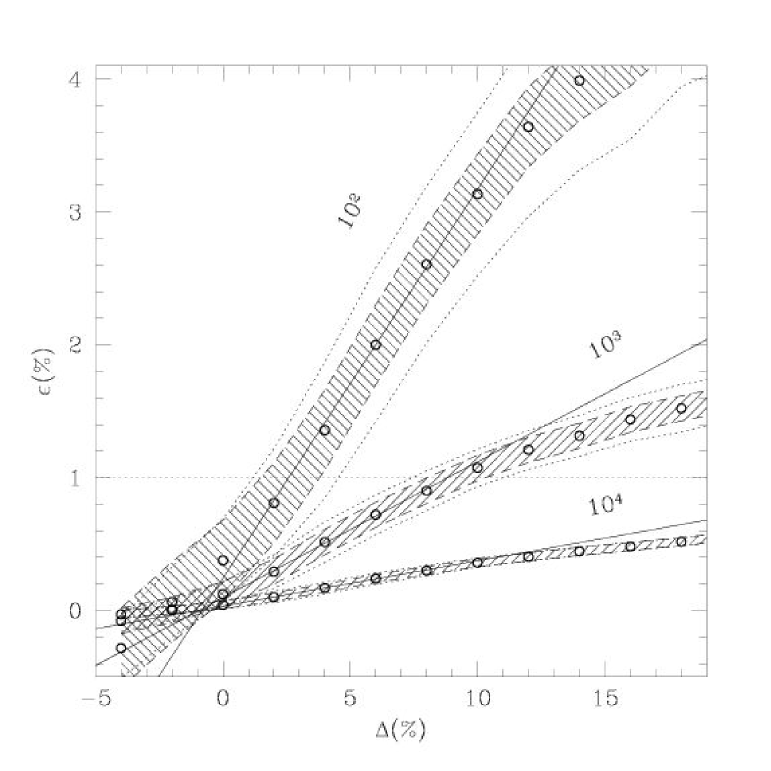
Figure 8: Errors on the estimated sky background $I_{sky}$ as a function of $\Delta$ (see text) from numerical simulations for three different sky background levels (10², 10³ and 10⁴ electrons). The continuous lines represent linear least squares fits in the range $0\leq\Delta\leq 10$, while the circles are the average (systematic) errors. Each point is the result of 5000 simulations. The dashed and dotted lines indicate the RMS random errors computed from the simulations and Eq. 11 ($N_{eff}=1000$) respectively. The horizontal dotted line is placed at $\epsilon_{max}$=1%.

A clear result emerges from Fig. 8: the $\Delta$ parameter is effective in estimating the systematic error and hence gives a statistically significant criterion to decide whether a sub-window can be considered as unperturbed or not. In order to have a simple description of the behaviour of $\langle\epsilon\rangle$ as a function of $\Delta$, we have performed a linear fitting of the simulated results in the range $0\leq\Delta\leq 10$ (see Fig. 8, continuous lines). Actually $\langle\epsilon\rangle$ tends to bend for larger values of $\Delta$ and this has the effect that our linear fitting slightly overestimates the value of $\langle\epsilon\rangle$. This is not a problem, since in this sense the criterion we are going to establish is just more restrictive. As expected, the slope of the $\Delta,\langle\epsilon\rangle$ relation is inversely proportional to the signal-to-noise ratio of the sky background. The best fit gives the following result:

$$\langle\epsilon\rangle=\frac{3.3}{\sqrt{I_{sky}}}\;(\Delta+0.96)$$ (15)

where $I_{sky}$ is given in electrons and $\Delta,\epsilon$ are expressed as percentage values. The fact that for $\Delta$=0 $\langle\epsilon\rangle\neq$0 is due to the following effect. When the sky background is contaminated by faint stars, whose maximum intensity is comparable to $\sqrt{I_{sky}}$, the mode and the width of the intensity distribution increase in such a way that $\Delta$ tends to be small, while the effective error is not.

We can now use the total maximum error $\epsilon_{max}$ to fix a limit on $\Delta$ below which we can consider a given intensity distributions as practically unperturbed. Since the distribution of random errors around the systematic deviation is Gaussian, we can conservatively assume $\epsilon_{max}\simeq\mid\langle\epsilon\rangle\mid+3\sigma_{\langle I\rangle}$. Using Eq. 15 for $\Delta$ one gets

$$\Delta_{max}=0.9\;\sqrt{\langle I\rangle}\;\left[\frac{\epsilon_{max}}{3}-\sigma_{\langle I\rangle}\right]-0.96$$ (16)

where $\sigma_{\langle I\rangle}$ is given by the adopted mode estimator. As it is shown in Sec. 3, this can be approximated by Eq. 11 with $N_{eff}$=1000, which gives the following expression:

$$\Delta_{max}=\frac{\sqrt{\langle I\rangle}}{3.3}\;\epsilon_{max}\;-1.9$$ (17)

The critical value for $\Delta$ depends of course on the accuracy one wants to reach in the estimate of the background intensity. For a typical value of $\epsilon_{max}$=1%, $\Delta_{max}$ is 1.1, 7.7 and 28.4% for sky levels of 10², 10³ and 10⁴ electrons respectively.

Once all sub-windows in an input image have been analysed with the criterion we have just discussed, a first sky brightness guess can be obtained using the median of all selected values. This has the effect of excluding cases like those produced by occulting masks inserted in the focal plane. In fact, to avoid strong saturation effects, FORS instruments allow the user to place a number of movable blades on specific positions of the focal plane. The height of these blades is about 20^′′, which correspond to 100 px when the SR collimator is used. When the occulted regions are larger than the adopted sub-window size, there is a chance that such areas pass the $\Delta$-test. Since the counts in those regions are very low, the median always removes them successfully, provided that the occulted fraction of the field of view is not larger than 50%, a condition which is always fulfilled.

After this selection is done, the only background fluctuations which are expected to be left in the remaining sub-windows are due to a non perfect flat-fielding. In fact, as we have mentioned in the introduction, the use of twilight flats introduces large scale gradients, which produce maximum peak-to-peak deviations of 6% from perfect flatness (see also next section). For this reason, we have decided to operate a further refinement, choosing only those $n_{g}$ sub-windows which deviate less than 3% from the median value. The final estimate of the background intensity $I_{sky}$ is eventually obtained computing the weighted mean $I_{sky}=\sum_{j=1}^{n_{g}}\langle I\rangle_{j}\;w_{j}/\sum_{j=1}^{n_{g}}w_{j}$, ($w_{j}=1/\sigma^{2}_{\langle I\rangle}$). To allow for a statistically significant result, we have imposed that $n_{g}\geq$5 in our automatic procedures. If this condition is not met, then the input frame is considered as unsuitable for sky background measures and rejected. This has the effect of operating a first rough filtering on the input data. To be conservative, $n_{g}$ is logged together with the other relevant parameters, and a further and more restrictive selection is always possible.

Intensive tests with real data, as discussed in the next section, have shown that the set of selection criteria we have discussed make the method reliable, robust and suitable to be implemented in a fully automatic procedure.

5 Testing the method on real data

The method we have just outlined has been tested on a sample of 4678 FORS1 reduced frames, obtained with different filters between April 1, 2000 and September 30, 2001. For each input frame the results relative to all 36 sub-windows have been logged and this has allowed us to build-up a sample with more than 168,000 entries, each of which has been flagged according to the results of the $\Delta$-test. The basic results are shown in Fig. 9, where we have plotted the measured noise (corrected for the read-out noise) as a function of the expected Poissonian noise. The solid line traces the locus where the two noises have the same value, while the dashed one indicates the limit on the measured noise imposed by Eq. 17. All sub-windows lying below the latter line would be selected for sky background estimates.

The fraction of selected windows is plotted in the upper panel of the same figure, again as a function of the expected noise. As one can see, for noise values of less than 20 electrons (or background intensities smaller than $\sim$400 electrons), this fraction is very low. For larger intensities, it reaches a roughly constant value of 80%. This means that basically all frames with $\langle I\rangle\leq 400$ electrons will be rejected. In the adopted test sample, this however accounts for 11% of total number of frames only. From the test sample we can conclude that, on average, 86.5% of FORS1 frames are suitable for sky-background measurements, 95% of which have $n_{g}\geq$12.

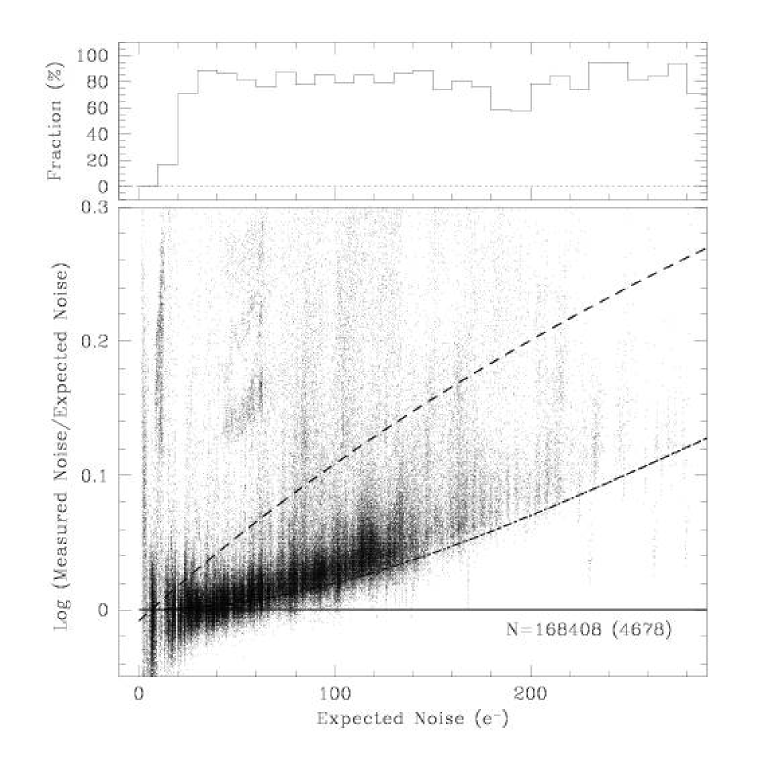
Figure 9: Comparison between the expected and measured noises on a sample of more than 4600 FORS1 images. Each point refers to a single sub-window. The solid line indicates the locus where the expected noise equals the measured one, while the dashed line traces the limit set by Eq. 17. The dashed-dotted line indicates the expected global noise generated by the photon statistics and the flat-fielding correction for a typical FORS1 configuration (see text for more details). The upper panel shows the fraction of sub-windows which passed the $\Delta$-test as a function of the expected noise.

An interesting feature visible in Fig. 9 is the systematic trend shown by the minimum measured noise. In fact, this tends to deviate more and more from the expected Poissonian noise for background values larger than $\sim$10⁴ electrons. This effect is explained by the following considerations. FORS1 master sky flat-fields are usually obtained by the combination of $N_{F}$=3 twilight sky flats, which have typical exposure levels of $I_{F}\sim$3.5$\times$10⁴ electrons. The resulting noise on the combined frame is usually negligible with respect to the noise present in the science frame to be corrected. When the background exposure level reaches high values, this is no longer true and the noise added by the flat-fielding process becomes significant. The expected global noise is in fact given by $\sigma^{2}=\sigma_{p}^{2}+I_{sky}^{2}/(N_{F}\;I_{F})$, where $I_{sky}$ is the background level in the input science frame. This law gives a fair reproduction of the observed behaviour, as it is shown in Fig. 9 (dashed-dotted line), where we have used the typical values of $I_{F}$ and $N_{F}$ quoted above. The few data points lying below this line are generated by observations obtained with the low gain mode ($\sim$0.3 ADU electron^-1), for which $I_{F}$ is about a factor of 2 larger than in the high gain mode ($\sim$0.6 ADU electron^-1) , which is also the standard for FORS1 imaging. In principle, when computing $\Delta$, one could correct the measured noise for the flat-fielding effect. In practice, at an exposure level of 5$\times$10⁴ electrons the correction on the measured noise is of the order of 20% and hence a very small number of sub-windows which are rejected by the $\Delta$ criterion would move to the safe region (see Fig. 9). Furthermore, 90% of all sub-windows included in the test sample have a background intensity smaller than 2$\times$10⁴ electrons. At this level, the correction amounts to about 10% only. For this reason we have decided to ignore the flat-fielding effect when evaluating the deviation from the pure Poissonian noise.

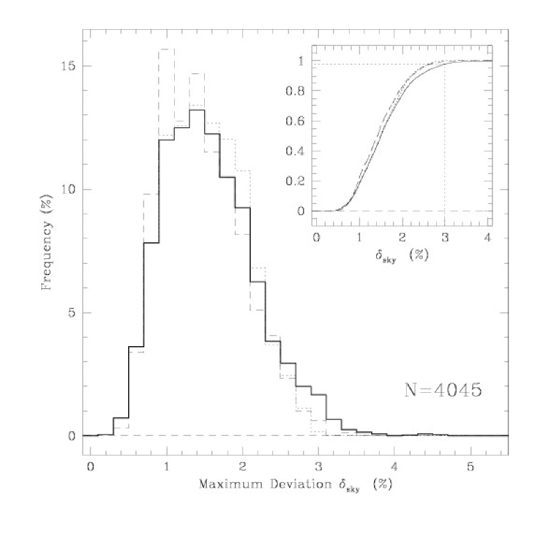
Figure 10: Maximum deviations from the sky background weighted mean in all frames which passed the $\Delta$-test. Solid line indicates the data from all sub-windows, the dotted line refers to the selected windows and the dashed line corresponds to the cases where $n_{g}$=36. The upper right insert shows the cumulative functions with the same line codings.

As we have mentioned (see also Sec. 3 for more details), the maximum formal errors on the mode estimate within the sub-windows are always smaller than 1%. Therefore it is clear that the major contribution to the uncertainty on the final background estimate is due to the non perfect flat-fielding, which introduces smooth large scale gradients in the reduced images. Due to the systematic nature of the effect, it does not make any statistical sense to adopt the formal error on the weighted mean to estimate this uncertainty and for this reason we have preferred to use the maximum deviation $\delta_{sky}$ measured in the $n_{g}$ selected windows. Of course, when $n_{g}\ll$36 and all the accepted sub-windows are concentrated in a portion of the frame, the use of $\delta_{sky}$ can lead to an error underestimate. In the case of our test sample, this effect is present for $n_{g}\lesssim$10, where the estimated error is a factor of two smaller than for larger $n_{g}$ values. Since the large majority of our data had $n_{g}>$12, this does not affect significantly our error estimates. This effect can be anyway reduced adopting larger values for the minimum number of sub-windows that must survive the $\Delta$-test.

The results produced applying our method to the test sample are shown in Fig. 10, where we present the distribution of $\delta_{sky}$ derived from the 4045 images which passed the $\Delta$-test. The solid line refers to the results one obtains using all windows which passed the $\Delta$-test, while the dotted line corresponds to the values obtained from the $n_{g}$ selected windows only. While the latter by definition drops to 0 at $\delta_{sky}$=3%, the former shows also the deviating cases at larger $\delta_{sky}$ which are, however, less than 3% of total. We emphasise that 20% of the measurements have $\delta_{sky}\leq$1%, while this fraction grows to 77.5% for $\delta_{sky}\leq$2%. The median value in the whole sample is 1.5%, which can be regarded as the typical maximum error in our measurements. It is finally interesting to note that the maximum error distribution one obtains using only those cases where all sub-windows are used for the final estimate ($n_{g}$=36, 1594 images, 39.5% of total) is not very different from the one which corresponds to the general case (Fig. 10, dashed line). Since the images for which all 36 sub-windows are selected are bona fide not affected by significant contamination, this confirms that the $\delta_{sky}$ distribution we observe is really due to large scale gradients and not to contaminated sub-windows which escaped the $\Delta$-test.

The efficiency of the method in recognising critical cases has been checked directly, with a visual inspection of a large number of cases included in the test sample. The conclusion is that the method is reliable and does not lead to artificial over-estimates of the sky background. As an example of these capabilities, in Fig. 11 we present a critical case drawn from our data sample: an $R$-band image of interacting galaxies. The boxes indicate the sub-windows which have passed the $\Delta$-test and which would be used for the first estimate. The lowest contour was traced at the 5 sigma level of the sky background (manually measured on a star-free area in the right upper corner). All selected sub-windows lie outside this contour, which reasonably defines the region where the galaxies certainly contribute to the background. As a matter of fact, there is a gradient within the accepted sub-windows, but the peak-to-peak difference is about 3% only, a value which is still consistent with the flat-fielding accuracy. As expected, all critical regions are disregarded. The final sky brightness is computed using the weighted mean on 23 sub-windows. It is interesting to note that even though some sub-windows include outer parts of the galaxies, the background value computed using our algorithm is fully consistent with that of visually selected object-free regions.

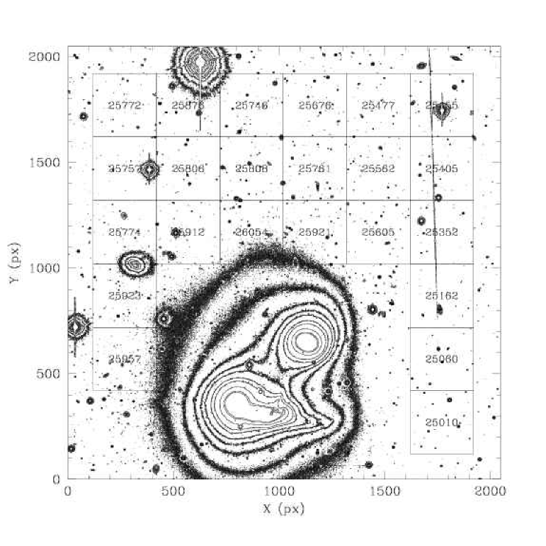
Figure 11: An example of a critical case: a group of interacting galaxies. The original 660 seconds image was taken in the R band on 03-05-2000, using the SR collimator (0″. 2 pixel^-1). The lowest contour was set at a 5 sigma level above the minimum sky background (measured in the upper right corner). Marked boxes indicate the sub-windows which were automatically judged as suitable for sky background determination according to our method; the number in each box shows the estimated sky background in electrons. The strip on the right side is a satellite trail.

6 Conclusions

In this paper we have presented a numerical algorithm to estimate the sky background in CCD imaging data. Due to the practical purpose this technique was designed for, we have optimized its implementation for FORS1; however, the algorithm is based on very general assumptions and it can be used for any CCD imager with a sufficiently wide field of view ($\geq$ 5${}^{\prime}\times$5^′).

The fulfilment of this requirement, coupled to the large size of the detectors currently available, allows one to estimate the mode of the image intensity distribution directly from its histogram, with a typical accuracy of 1% or better (Sec. 3). In order to identify suitable regions within the image, the analysis is performed in smaller sub-windows which, in the case of FORS1, have a size of 1${}^{\prime}\times$1^′ and include 9$\times$10⁴ pixels. The possible presence of contaminating objects within these areas is detected studying the shape of the intensity distribution.

The criterion to reject such regions from the final sky background estimate, that we have indicated as $\Delta$-test, has been established via numerical simulations and it is based on the effects that perturbing objects have on the left wing of the local intensity distribution (Sec. 4).

The method has been designed to be robust and reliable under a large variety of conditions. The tests have shown that it can be safely used in fully automatic procedures (Sec. 5) and therefore it is suitable for processing large data volumes. The tests on real images have also shown that the final accuracy is determined mostly by the flat-fielding quality on large scales. In the specific case of FORS1 this is typically of the order of 2$-$3% (peak-to-peak) across the whole field of view. This sets a lower limit for the study of night sky brightness variations on the arcminutes scale, since they cannot be disentangled from those artificially induced by the flat-fielding process.

As far as the contribution of faint stars to the sky background is concerned, the simulations show that our algorithm is undisturbed by the presence of stellar objects with peak intensity $I_{*}\geq 5\sigma_{p}$. In the case of sky background dominated images, the magnitude of those sources is given by the following expression:

$$m_{f}=m_{0}-2.5\;log\left[5.7\;\frac{FWHM^{2}}{p^{2}}\right]-1.25\;log\left[\frac{r_{sky}}{t}\right]$$ (18)

where $m_{0}$ is the photometric zero point in a given passband, $p$ is the pixel scale (in arcsec px^-1), $r_{sky}$ is the sky background rate (in e^- s^-1), $t$ is the exposure time (in seconds) and $FWHM$ is the seeing (in arcsec). For example, FORS1 $V$ frames obtained through the SR collimator ($p$=0.2 arcsec px^-1) become sky background dominated in about 25 seconds (see Patat patat (2003)). With this exposure time, a seeing of 1^′′ and the typical FORS1 zero point in the $V$ passband ($m_{0}\simeq$28), Eq. 18 gives $m_{f}\sim$22.8, which is about 10 magnitudes fainter than the value for typical photoelectric sky brightness surveys (Walker walker88 (1988)). Such faint objects contribute to less than 1% to the total brightness (Roach & Gordon roachgordon (1973)) and therefore we can conclude that our method is practically free from being biased by the inclusion of faint foreground point sources.

Finally, to asses the speed performance of our algorithm, we have compiled and executed a C coded version on a moderately fast Linux PC (Penthium III 500 MHz, 256 MB RAM). On such a machine, the analysis of a 2048$\times$2048 px image requires less than 6 seconds, making it suitable for on-line processing.

The method we have presented here has been extensively used in the ESO-Paranal night sky brightness survey, which made use of more than 3900 $UBVRI$ FORS1 frames collected from April 2000 to September 2001. The results are presented and discussed in Patat (patat (2003)).

- (1) Benn, C. R. & Ellison, S. L. 1998, La Palma Technical Note n.115
- (2) Bertin, E. & Arnouts, S. 1996, A&A, 117, 393
- (3) Roach, F.E. & Gordon, J.L. 1973, The light of the Night Sky, D. Reidel Publ. Company, Dordrecht
- (4) Huber, P. J. 1981, Robust statistics, John Wiley & Sons, p. 107
- (5) Kendall, M. & Stuart, K. 1977, The Advanced Theory of Statistics, Vol. 1. (Charles Griffin & Co., London)
- (6) Leinert, Ch., Bowyer, S., Haikala, L.K., et al. 1998, A&AS, 127, 1
- (7) Lupton, R. 1993, Statistics in Theory and Practice, p. 6, Princeton University Press
- (8) Patat, F. 2003, A&A, in press, astro-ph/0301115
- (9) Ratnatunga, K. U. & Newell, E. B. 1984, AJ, 89, 176
- (10) Spiegel, M. R. 1988, Statistics, 2nd. ed., McGraw-Hill
- (11) Stetson, P.B., 1987, PASP, 99, 191
- (12) Szeifert, T. 2002, FORS1+2 User’s Manual, VLT-MAN-ESO-13100-1543, Issue 2.3
- (13) Walker, M. F. 1988, PASP, 100, 496