Galactic Halos of Fluid Dark Matter

Abstract

Dwarf spiral galaxies – and in particular the prototypical DDO 154 – are known to be completely dominated by an unseen component. The putative neutralinos – so far the favored explanation for the astronomical dark matter – fail to reproduce the well measured rotation curves of those systems because these species tend to form a central cusp whose presence is not supported by observation. We have considered here a self–coupled charged scalar field as an alternative to neutralinos and investigated whether a Bose condensate of that field could account for the dark matter inside DDO 154 and more generally inside dwarf spirals. The size of the condensate turns out to be precisely determined by the scalar mass $m$ and self–coupling $\lambda$ of the field. We find actually that for $m^{4}/\lambda\sim$ 50 – 75 eV⁴, the agreement with the measurements of the circular speed of DDO 154 is impressive whereas it lessens for larger systems. The cosmological behavior of the field is also found to be consistent – yet marginally – with the limits set by BBN on the effective number of neutrino families. We conclude that classical configurations of a scalar and self–coupled field provide a possible solution to the astronomical dark matter problem and we suggest further directions of research.

I Introduction

After many years of global consensus on the fact that dark matter consists in Weakly Interacting Massive Particles (WIMPs) – like, for instance, the lightest neutralino in the Minimal Supersymmetric Standard Model (MSSM) – there is still no strong evidence in favor of WIMPS, neither from bolometer experiments designed for direct detection, nor from the observation of cosmic rays, a fraction of which could consist in WIMPs annihilation products. This absence of experimental constraints on dark matter from the particle physics side leaves the door wide open for alternative descriptions of the hidden mass of the Universe.

Moreover, in the past three years, there has been a lot of controversy concerning the small–scale inhomogeneities of the WIMPs density. Indeed, many recent N–body simulations of structure formation in the Universe suggested that any dark matter component modelized as a gas of free particles – such as WIMPs – tends to cluster excessively on scales of order 1 kpc and smaller. This would result in cuspy density profiles at galactic centers, while most rotation curves indicate a smooth core density [1]. Many galaxies even seem to be dominated by baryons near their center, with a significant dark matter fraction only at large radii. This clearly contradicts the results from current N–body simulations, in which the dark matter density is strongly enhanced at the center of the halo with respect to its outskirts.

This argument was attacked by Weinberg and Katz [2], who stressed the importance of including the baryon component in N–body simulations. Indeed, the baryon dissipative effects could be responsible for a smoothing of the central dark matter cusp in the early Universe. This possible solution to the dark matter crisis was discarded later by Sellwood [3], who found opposite results in his simulation.

Apart from the central cusp problem, N–body simulations raised some secondary issues [1]. First, a clumpy halo could generate some tidal effects that could break the spatial coherence of the disk. Second, the predicted number of satellite galaxies around each galactic halo is far beyond what we see around the Milky Way. Third, the dynamical friction between dark matter particles and baryons should freeze out the spinning motion of baryonic bars in barred galaxies. All these arguments are still unclear, because they seem to depend on the resolution under which simulations are carried [4, 5], and also because of our ignorance of what could be the light–to–mass ratio inside small dark matter clumps. In addition, the predicted number of satellite galaxies doesn’t seem to be in contradiction with constraints from microlensing [6].

Should these various problems be confirmed or not, it sounds reasonable to explore alternatives to the WIMPs model, or more generally speaking, to any description based on a gas of free particles. This can be done in various ways: for instance, one can introduce some deviations from a perfect thermal phase–space distribution [7], or add a self–coupling between dark matter particles [8]. A more radical possibility is to drop the assumption that dark matter is governed by the laws of statistical thermodynamics. This would be the case if dark matter consisted in a classical scalar field, coherent on very large scales, and governed by the Klein–Gordon equation of motion.

This framework should be clearly distinguished from other models of bosonic dark matter, like those based on heavy bosons – for instance, sneutrinos – or axions. In the first case, the Compton wavelength $\hbar/(mc)$ of an individual particle is much smaller than the typical interparticle distance while in the second case, for axion masses of order $10^{-6}$ eV, it is still much smaller than the typical size of a galaxy. So, in these examples, the bosons can be described on astronomical scales like a gas of free particles in statistical equilibrium. It follows that the halo structure cannot be distinguished from that of standard WIMPs.

A coherent scalar field configuration governed by the Klein–Gordon and Einstein equations is nothing but a self–gravitating Bose condensate. Such condensates span over scales comparable to the De Broglie wavelength, $L=\hbar/p$. In the case of free bosons – i.e., with a quadratic scalar potential – the momentum $p$ is of order $mv_{\rm esc}$ where $v_{\rm esc}$ is the escape velocity from the system. Typical examples are boson stars [9, 10, 11, 12], for which the characteristic orders of magnitude discussed in the literature are, for instance, $m\sim 10$ GeV and $v_{\rm esc}\sim c$, leading to a radius as tiny as $L\sim 10^{-14}$ cm. Even for axions, which have a much smaller mass and an escape velocity given by the motion of stars in a galaxy – $v_{\rm esc}\sim 100$ km/s – the De Broglie wavelength is only of order $L=100$ km, so that on galactic scales, the medium can be treated as a gas. In order to obtain a galactic halo described by the Klein–Gordon equation, one should consider masses of order $m=\hbar/(Lv_{\rm esc})$ where $v_{\rm esc}\sim 100$ km/s and $L\sim 10$ kpc. This yields $m\sim 10^{-23}$ eV. Such an ultra–light scalar field was called “fuzzy dark matter” by Hu [13], who discussed its overall cosmological behavior. In some previous works, we focused on a variant of this model in which the ultra–light scalar field is complex – then, the conserved number associated with the $U(1)$ global symmetry helps in stabilizing the condensate against fragmentation [10, 12]. In [14] – thereafter Paper I – we compared the rotation curves predicted by this model with some data from spiral galaxies. In [15] – thereafter Paper II – we simulated the cosmological evolution of the homogeneous background of such a field. The model seems to be quite successful in explaining the rotation curves, but it has two caveats. First, such a low mass is very difficult to implement in realistic particle physics models. The second problem is related to the fact that because of the $U(1)$ symmetry, the field carries a conserved quantum number. As explained in Paper II, the value derived from cosmological considerations for the density of this quantum number does not seem consistent with that inferred from astrophysical arguments.

These caveats motivate the introduction of a quartic self–coupling term in the scalar potential. In that case, it is already known from boson stars that for the same value of the mass, the self–coupling constrains the field to condensate on much larger scales [16, 12] – the size of the self–gravitating configurations is still given by $L=\hbar/p$, but in presence of a self–coupling, the momentum cannot be identified with $mv_{\rm esc}$. Then, without recurring to ultra–light masses, we may still describe the galactic halos with a Bose condensate. A massive scalar field with quartic – or close to quartic – self–coupling was proposed as a possible dark matter candidate by Peebles, who called it “fluid dark matter” [17]. In this paper, we will study a variant of fluid dark matter in which the quartically self–coupled massive scalar field is complex, still for stability reasons. Some cosmological properties of such a field were already discussed in [19].

We will focus mainly on galaxy rotation curves, assuming that the dark matter halos are the self–gravitating, aspherical and stable equilibrium configurations of our scalar field in the presence of a baryonic matter distribution – stellar disk, HI gas, etc… We will present here the first solution of this problem. However, we should stress that some different models in which the rotation curves are also seeded by a coherent scalar field were studied previously by Schunk [20] – with a vanishing scalar potential, Goodman [21] – with a repulsive self-interaction, Matos et al. [22], Nucamendi et al. [23], Wetterich [24], Urena-Lopez and Liddle [25]. In some of these papers, and also in many other recent proposals – see for instance [26] – the main goal is to try to solve simultaneously the dark energy and dark matter problems, assuming that a quintessence field can cluster on galactic scales. This raises some subtle issues, like the existence of a scale–dependent equation of state. At the present stage, we do not have such an ambition, and we will focus only on the dark matter problem.

In section II, we write the Einstein and the Klein–Gordon equations which govern the scalar field and the gravitational potential distributions in the presence of a given baryonic matter density. We will see that these equations can be combined into a single non–linear Poisson equation. The solutions are technically difficult to find, first, due to the non–linearity, and second, because some boundary conditions are given at the center, some others at infinity. So, it is not possible to follow a lattice approach, in which one would start from a particular point and integrate numerically grid point by grid point. However we present in section III a recursive method which allows to find all the exact solutions after a few iterations. In section IV, we compare the galaxy rotation curves obtained in this way with some observational data. We lay a particular emphasis on the dwarf spiral galaxy DDO 154, for which the rotation curve is among the most difficult to explain with usual dark matter profiles. We will see that a mass–over–self–coupling ratio $m^{4}/\lambda\simeq 50$ $({\rm eV})^{4}$ provides a very good fit to the DDO 154 rotation curve – however at the expense of poor fits to the largest spiral galaxies. Because the scalar field condensates inside the gravitational potential wells of baryons and strengthens them, the question of its effects on the inner dynamics of the solar system naturally arises. We derive in section V the modification of the solar attraction in the presence of the self–interacting scalar field under scrutiny and show that an anomalous acceleration appears that is constant and that points towards the Sun. We investigate the limit set on our model by the Pioneer radio data. In Paper II, we studied the cosmological behavior of a homogeneous scalar field that was assumed to play the role of dark matter at least from the time of matter–radiation equality until today. This analysis is updated in section VI where we specifically assume $m^{4}/\lambda\simeq 50$ $({\rm eV})^{4}$. Such a large value point towards a large total density of the Universe during radiation domination which is at the edge of the current bounds set in particular by BBN on cosmological parameters. The last section is devoted to a discussion of the strong and weak aspects of our alternative dark matter model. We finally suggest some further directions of investigation beyond the simple but restrictive framework of isolated bosonic configurations.

II Gravitational behavior

The complex scalar field $\phi$ under scrutiny in this article is associated to the Lagrangian density

$${\cal L}\;=\;g^{\mu\nu}\,\partial_{\mu}\phi^{\dagger}\,\partial_{\nu}\phi\;-\;V\left(\phi\right)\;\;,$$ (1)

where the $U(1)$ invariant potential $V$ includes both quadratic and quartic contributions

$$V\left(\phi\right)\;=\;m^{2}\,\varphi^{\dagger}\phi\;+\;\lambda\,\left\{\phi^{\dagger}\phi\right\}^{2}\;\;.$$ (2)

The gravitational behavior of the system follows the standard GR equations whilst the field $\phi$ satisfies the Klein–Gordon equation

$${\displaystyle\frac{1}{\sqrt{-g}}}\;\partial_{\mu}\left\{\sqrt{-g}\,g^{\mu\nu}\,\partial_{\nu}\phi\right\}\;+\;{\displaystyle\frac{\partial V}{\partial\phi^{\dagger}}}\;=\;0\;\;,$$ (3)

where $g_{\mu\nu}$ denotes the metric. We would like to investigate to which extent the scalar field $\phi$ may account for the dark matter inside galaxies. The problem simplifies insofar as the gravitational fields at stake are weak and static. In this quasi–Newtonian limit of general relativity, deviations from the Minkowski metric $\eta_{\mu\nu}=diag\left\{1,-1,-1,-1\right\}$ are accounted for by the perturbation tensor $h_{\mu\nu}$ – from now on, we use the convention $c=1$. The Newtonian gravitational potential $\Phi=h_{00}/2$ is actually a small quantity of order $v_{\rm esc}^{2}\sim 10^{-7}-10^{-6}$, where $v_{\rm esc}$ denotes the escape velocity. Our analysis is based on an expansion up to first order in $\Phi$. The baryonic content of galaxies is described through the energy–momentum tensor

$$T^{\mu\nu}\;=\;\left(\mbox{$\rho_{\rm\,b}$}+\mbox{$P_{\rm\,b}$}\right)U^{\mu}U^{\nu}\;-\;\mbox{$P_{\rm\,b}$}\,g_{\mu\nu}\;\;,$$ (4)

where $U^{\mu}=\{1,\vec{v}\}$. Baryons behave as dust with non–relativistic velocities. Actually, because galaxies are virialized systems – hence the assumption of static gravitational fields – the spatial velocity $v$ is a small quantity of order $v_{\rm esc}\sim\sqrt{\Phi}$. The kinetic pressure–to–mass density ratio is even more negligible since $\mbox{$P_{\rm\,b}$}/\mbox{$\rho_{\rm\,b}$}\sim v^{2}\sim v_{\rm esc}^{2}\sim\Phi\ll 1$. We are interested in classical configurations where the field $\phi$ is in a coherent state such as

$$\phi\left\{\vec{x},t\right\}\;=\;{\displaystyle\frac{\sigma\left(\vec{x}\right)}{\sqrt{2}}}\,\exp\left(-\,i\,\omega\,t\right)\;\;.$$ (5)

Indeed, one can prove that all stable spherically symmetric configurations can be parameterized in that way [10]. The time–derivative $\partial_{0}\phi$ equals $-i\,\omega\,\phi$, whereas the space–derivative $\partial_{i}\phi$ is of order $\phi/L$ where $L$ is the physical length of the configuration. That length – which is related to the parameters $m$ and $\lambda$ of the potential – is required to be $\sim$ 1 – 100 kpc to account for the galactic dark matter. On the other hand, we shall see later that $\omega$ is very close to the mass $m$, which is numerically found to be in the ballpark of a fraction of eV. We readily infer a ratio

$${\displaystyle\frac{\partial_{i}\phi}{\partial_{0}\phi}}\sim{\displaystyle\frac{1}{m\,L}}\;=\;6.4\times 10^{-27}\;\left\{{\displaystyle\frac{1\,{\rm eV}}{m}}\right\}\;\left\{{\displaystyle\frac{1\,{\rm kpc}}{L}}\right\}\;\;.$$ (6)

So, the space derivative $\partial_{i}\phi$ of the scalar field can be safely neglected throughout the analysis.

In its weak–field limit, general relativity becomes a gauge theory. By conveniently choosing the gauge of harmonic coordinates in which the metric perturbation $h_{\mu\nu}$ satisfies the condition

$$\partial_{\mu}h^{\mu}_{\;\;\alpha}\;=\;\frac{1}{2}\,\partial_{\alpha}\left\{h^{\mu}_{\;\;\mu}\right\}\;\;,$$ (7)

the GR equations simplify into

$$\Box h_{\mu\nu}\;=\;-\,16\,\pi\,G\,S_{\mu\nu}\;\;.$$ (8)

The effective source $S_{\mu\nu}$ is related to the energy–momentum tensor $T_{\mu\nu}$ through

$$S_{\mu\nu}\;=\;T_{\mu\nu}\,-\,\frac{1}{2}\,g_{\mu\nu}\,T^{\lambda}_{\;\;\lambda}\;\;.$$ (9)

In the propagation eq. (8), the source $S_{\mu\nu}$ is computed in flat space while the metric perturbation $h_{\mu\nu}$ is of order $\Phi$. If the dark matter inside galaxies is understood as some classical configuration of the field $\phi$, $S_{\mu\nu}$ should take into account both baryonic population – stars and gas – and scalar condensate. In the Newtonian limit where gravito–magnetic effects are disregarded, the non–relativistic velocities of baryons can be neglected. The only non–vanishing components of the baryonic source tensor are

$$S^{\rm\;b}_{00}\;=\;{\displaystyle\frac{\mbox{$\rho_{\rm\,b}$}}{2}}{\hskip 28.45274pt}{\rm and}{\hskip 28.45274pt}S^{\rm\;b}_{ij}\;=\;-\,\eta_{ij}\,{\displaystyle\frac{\mbox{$\rho_{\rm\,b}$}}{2}}\;\;.$$ (10)

Assuming that eq. (5) describes the scalar field configuration and disregarding the space–derivatives $\partial_{i}\phi$ leads to the source components

$$S^{\;\varphi}_{00}\;=\;\omega^{2}\sigma^{2}\,-\,V{\hskip 28.45274pt}{\rm whilst}{\hskip 28.45274pt}S^{\;\varphi}_{ij}\;=\;-\,\eta_{ij}\,V\;\;,$$ (11)

where the potential is

$$V\left(\sigma\right)\;=\;{\displaystyle\frac{m^{2}}{2}}\,\sigma^{2}\;+\;{\displaystyle\frac{\lambda}{4}}\,\sigma^{4}\;\;.$$ (12)

The well–known solution of the Lienard and Wiechert retarded potentials satisfies the propagation eq. (8). We readily conclude that the metric does not contain any space–time component $h_{0i}$ and may be expressed at this stage as

$$d\tau^{2}\;=\;\left(1\,+\,2\Phi\right)dt^{2}\;-\;\left(1\,-\,2\Psi\right)\delta_{ij}\,dx^{i}dx^{j}\;\;,$$ (13)

where the static potentials $\Phi$ and $\Psi$ are given by integrals over the source distribution ${\cal D}$ of the baryonic and scalar mass densities

$$\Phi(\vec{x})\;=\;-\,G\,{\displaystyle\int_{\cal D}}\,{\displaystyle\frac{d^{3}\vec{y}}{|\vec{x}-\vec{y}|}}\,\left\{\mbox{$\rho_{\rm\,b}$}(\vec{y})+\mbox{$\rho^{\prime}_{\phi}$}(\vec{y})\right\}\;\;,$$ (14)

and

$$\Psi(\vec{x})\;=\;-\,G\,{\displaystyle\int_{\cal D}}\,{\displaystyle\frac{d^{3}\vec{y}}{|\vec{x}-\vec{y}|}}\,\left\{\mbox{$\rho_{\rm\,b}$}(\vec{y})+\mbox{$\rho^{\prime\prime}_{\phi}$}(\vec{y})\right\}\;\;.$$ (15)

The densities $\rho^{\prime}_{\phi}$ and $\rho^{\prime\prime}_{\phi}$ are respectively defined by

$$\mbox{$\rho^{\prime}_{\phi}$}\;=\;2\,\omega^{2}\sigma^{2}\,-\,m^{2}\sigma^{2}\,-\,{\displaystyle\frac{\lambda}{2}}\,\sigma^{4}\;\;,$$ (16)

and

$$\mbox{$\rho^{\prime\prime}_{\phi}$}\;=\;m^{2}\sigma^{2}\,+\,{\displaystyle\frac{\lambda}{2}}\,\sigma^{4}\;\;.$$ (17)

The potentials $\Phi$ and $\Psi$ are different a priori. A careful inspection of the Klein–Gordon equation will eventually show that they are actually equal. The latter may be written as

$$\left(1\,-\,2\Phi\right)\,\ddot{\phi}\;-\;\left(1\,+\,\Phi\,-\,3\Psi\right)^{-1}\,\partial_{i}\left\{\left(1\,+\,\Phi\,-\,\Psi\right)\,\partial_{i}\phi\right\}\;+\;{\displaystyle\frac{\partial V}{\partial\phi^{\dagger}}}\;=\;0\;\;.$$ (18)

The space–dependent term is some 53 orders of magnitude smaller than its time–dependent counterpart and we can safely disregard it so that relation (18) simplifies into

$$\lambda\sigma^{2}\;=\;\left(1\,-\,2\Phi\right)\omega^{2}\,-\,m^{2}\;\;,$$ (19)

where the configuration (5) has been assumed. The scalar field is in a classical state that may be pictured as a Bose condensate on the boundaries of which the gravitational potential is

$$\Phi_{0}\;=\;\frac{1}{2}\left(1\,-\,{\displaystyle\frac{m^{2}}{\omega^{2}}}\right)\;\;.$$ (20)

Because the potential $\Phi_{0}$ is a small quantity, the pulsation $\omega$ is very close to the mass $m$. The scalar field essentially vanishes outside the condensate whereas its inner value is directly related to the gravitational potential $\Phi$ through

$$\lambda\sigma^{2}\;=\;2\,\left(\Phi_{0}-\Phi\right)\,\omega^{2}\;\simeq\;2\,\left(\Phi_{0}-\Phi\right)\,m^{2}\;\;.$$ (21)

This relation has important consequences. To commence, the densities $\mbox{$\rho^{\prime}_{\phi}$}=m^{2}\sigma^{2}\,\left\{1\,+\,3\Phi_{0}\,-\,\Phi\right\}$ and $\mbox{$\rho^{\prime\prime}_{\phi}$}=m^{2}\sigma^{2}\,\left\{1\,+\,\Phi_{0}\,-\,\Phi\,-\,2\Psi\right\}$ become both equal to $\mbox{$\rho_{\phi}$}\simeq m^{2}\sigma^{2}$ at lowest order in the potentials. Then $\Phi\equiv\Psi$ and the metric simplifies. It is straightforward to show that it readily satisfies the gauge condition (7). The scalar field density may be expressed as a difference between the gravitational potentials inside and on the boundary of the scalar field condensate

$$\mbox{$\rho_{\phi}$}\;=\;{\displaystyle\frac{2\,m^{4}}{\lambda}}\,\left(\Phi_{0}-\Phi\right)\,{\cal H}\left(\Phi_{0}-\Phi\right)\;\;,$$ (22)

where ${\cal H}(x)=1$ for $x>0$ and ${\cal H}(x)=0$ elsewhere. This leads to the Poisson equation

$$\Delta\Phi\,=\;4\,\pi\,G\,\mbox{$\rho_{\rm\,b}$}\;\;+\,8\,\pi\,G\,{\displaystyle\frac{m^{4}}{\lambda}}\,\left(\Phi_{0}-\Phi\right)\,{\cal H}\left(\Phi_{0}-\Phi\right)\;\;.$$ (23)

Inside the condensate, gravity turns out to be effectively modified by the presence of the scalar density $\rho_{\phi}$ whereas the conventional Poisson equation is recovered outside. Defining the Planck mass through $M_{\rm P}=1/\sqrt{G}$, we derive a typical scale of

$$L^{2}\;=\;{\displaystyle\frac{\lambda}{8\,\pi}}\,{\displaystyle\frac{M_{\rm P}^{2}}{m^{4}}}\;=\;{\displaystyle\frac{\Lambda}{m^{2}}}\;\;,$$ (24)

for the scalar field configurations in which we are interested. The dimensionless constant $\Lambda$ has been introduced by [16] in their analysis of self–interacting boson stars. The scale $L$ is related to the mass $m$ and the quartic coupling $\lambda$ through

$$L\;\simeq\;1.6\;{\rm kpc}\;\left\{{\displaystyle\frac{\lambda}{10^{-2}}}\right\}^{1/2}\;\left\{{\displaystyle\frac{1\,{\rm eV}}{m}}\right\}^{2}\;\;,$$ (25)

so that values of the mass in the ballpark of the eV may well be compatible with a size $L$ of order a few kiloparsecs. As already noticed by [16], the space–dependent term in the Klein–Gordon eq. (18) is actually suppressed by a factor of $\Lambda$ which, in our case, reaches values as large as $\sim 10^{53}$. The key feature of the scalar field configurations at stake is the existence of a unique scale $L$ that depends only on the parameters $m$ and $\lambda$ of the potential $V$.

A pure scalar field configuration may also be seen as a mere fluid with mass density $\rho_{\phi}$. The pressure $P_{\phi}$ may be derived from the space–space component $T_{ij}=-\,\eta_{ij}\,\mbox{$P_{\phi}$}$ of its energy–momentum tensor. This leads to

$$\mbox{$P_{\phi}$}\;=\;{\cal L}\;=\;g^{00}\,\dot{\phi}^{\dagger}\dot{\phi}\,-\,V\;\simeq\;{\displaystyle\frac{m^{4}}{\lambda}}\,\left(\Phi_{0}-\Phi\right)^{2}$$ (26)

inside the condensate where $\Phi\leq\Phi_{0}$. The corresponding equation of state boils down to

$$\mbox{$P_{\phi}$}\;=\;{\displaystyle\frac{\lambda}{4\,m^{4}}}\;\mbox{$\rho_{\phi}$}^{2}\;\;,$$ (27)

and features the generic polytropic form $P\,=\,K\,\rho^{\Gamma}$ where $\Gamma=1+1/n$ and $K={\lambda}/{4\,m^{4}}$ are constants. Spherical symmetric solutions of configurations in hydrostatic equilibrium are searched of the form $\rho/\rho_{C}=\Theta^{n}(z)$ and $P/P_{C}=\Theta^{n+1}(z)$ where $z=r/L$ is the dimensionless radius. The typical scale of the polytrope depends on the central density $\rho_{C}$ and pressure $P_{C}$ through

$$L^{2}\;=\;{\displaystyle\frac{(n+1)P_{C}}{4\,\pi\,G\,\rho_{C}^{2}}}\;\;,$$ (28)

whereas the generic function $\Theta$ satisfies the Lane–Emden equation

$${\displaystyle\frac{1}{z^{2}}}\,{\displaystyle\frac{d}{dz}}\left\{z^{2}\,{\displaystyle\frac{d\Theta}{dz}}\right\}\;=\;-\,\Theta^{n}\;\;,$$ (29)

with the initial conditions $\Theta(0)=1$ and $\Theta^{\prime}(0)=0$. In the scalar field case, the polytropic index is $n=1$ and the solution

$${\displaystyle\frac{\mbox{$\rho_{\phi}$}}{\mbox{$\rho_{\phi}$}_{C}}}\;=\;\Theta(z)\;=\;{\displaystyle\frac{\sin z}{z}}$$ (30)

readily obtains. It describes a spherical symmetric configuration where the scalar field alone is bound by its own gravity. The radius of the pure scalar field condensate is then $R=\pi\,L$ where the scale $L$ has already been derived in relations (24) and (25):

$$R\;=\;\pi\,L\;=\;\pi\left\{{\displaystyle\frac{K}{2\,\pi\,G}}\right\}^{1/2}\;\equiv\;\pi\left\{{\displaystyle\frac{\lambda}{8\,\pi\,G}}\right\}^{1/2}\,{\displaystyle\frac{1}{m^{2}}}$$ (31)

The effect of an aspherical distribution of baryons on the scalar field condensate will be examined in the next section.

III Resolution method

We would like to compute the gravitational potential $\Phi$ associated with any density of baryons $\rho_{b}$ in the galaxy, in the presence of a scalar field condensate. So, we need to solve eq. (23). The Heaviside function renders this equation strongly non–linear: different solutions have different surfaces where

$$\Phi(\vec{x})=\Phi_{0}\,,$$ (32)

so the sum of two solutions is not a solution. Nevertheless, it is possible to solve the equation with a recursive method. The idea is to start from an approximate solution $\Phi^{(0)}$, and to find $\Phi^{(n)}$ from the iterations

$$\Delta\Phi^{(n+1)}=4\pi G\rho_{b}+8\pi G\frac{m^{4}}{\lambda}\left(\Phi_{0}-\Phi^{(n)}\right)\,\,{\cal H}\!\left(\Phi_{0}\!-\!\Phi^{(n)}\right)\;\;.$$ (33)

If, for a judicious choice of $\Phi^{(0)}$, the $\Phi^{(n)}$’s converge towards a limit $\Phi^{(\infty)}$, then the latter will be an exact solution of (23).

We will always work in the approximation in which the baryonic density $\rho_{b}(\vec{x})$ is axially symmetric, continuous and vanishing at infinity. So, the induced gravitational potential should be

$$\left\{\begin{array}[]{l}{\rm axially~{}symmetric,}\\ {\rm continuous~{}and~{}twice~{}derivable,}\\ {\rm vanishing~{}at~{}infinity.}\end{array}\right.$$ (34)

We introduce a spherical coordinate system $(r,\theta,\varphi)$ where $(\theta=0)$ defines the symmetry axis. So, there will be no $\varphi$–dependence in the solutions, and a good way to find them is to perform a Legendre transformation. Let’s first illustrate this for the general Poisson equation:

$$\Delta\Phi(r,\theta)=S(r,\theta)\,,$$ (35)

where $S$ and $\Phi$ possess the properties of symmetry and continuity listed previously. If one decomposes the potential $\Phi$ and the source term $S$ into Legendre polynomials:

$$\Phi(r,\theta)=\sum_{l=0}^{+\infty}P_{l}(\cos\theta)\Phi_{l}(r)\,,$$ (36)

$$S(r,\theta)=\sum_{l=0}^{+\infty}P_{l}(\cos\theta)S_{l}(r)\,,$$ (37)

then the $S_{l}$’s are found from

$$S_{l}(r)=\frac{2l+1}{2}\int_{-1}^{+1}S(r,\theta)P_{l}(\cos\theta)d(\cos\theta)\;,$$ (38)

while the $\Phi_{l}$’s are the solutions of the linear set of equations

$$\frac{1}{r^{2}}\frac{d}{dr}\left(r^{2}\frac{d\Phi_{l}}{dr}\right)-\frac{l(l+1)}{r^{2}}\Phi_{l}=S_{l}\,.$$ (39)

The boundary conditions are given by the properties (34) for all $l$’s,

$$\frac{d}{dr}\Phi_{l}(0)=0\qquad{\rm and}\qquad\lim_{r\to+\infty}\Phi_{l}(r)=0\,.$$ (40)

So, in order to find the solution of eq. (39), one can first compute some Green functions $G_{l}$ that are continuous, null at infinity, with zero derivative at the center, and verifying

$$\frac{1}{r^{2}}\frac{d}{dr}\left(r^{2}\frac{\partial}{\partial r}G_{l}(r,u)\right)-\frac{l(l+1)}{r^{2}}G_{l}(r,u)=\delta(r-u)$$ (41)

where $\delta$ is the Dirac function. The unique answer is

$$G_{l}(r,u)=-\frac{u}{2l+1}\left\{\left(\frac{r}{u}\right)^{l}{\cal H}(u-r)+\left(\frac{r}{u}\right)^{-(l+1)}{\cal H}(r-u)\right\}\,.$$ (42)

Since $\displaystyle\Phi_{l}(r)=\int_{0}^{+\infty}S_{l}(u)G_{l}(u,r)du$, one finally finds

$$\Phi_{l}(r)=-\frac{r^{-(l+1)}}{2l+1}\int^{r}_{0}S_{l}(u)u^{l+2}du-\frac{r^{l}}{2l+1}\int^{+\infty}_{r}S_{l}(u)u^{1-l}du\,.$$ (43)

We can still use this Green function technique in our recursive method. Indeed, if $\Phi^{(n)}$ shares the properties (34), then we can identify the right-hand side of eq. (33) with $S(r,\theta)$, and find $\Phi^{(n+1)}$ using the method described above. Then $\Phi^{(n+1)}$ also shares the properties (34).

So, at each recursion step, we need to expand the right hand-side of eq. (33) in Legendre coefficients. Note that the $\Phi^{(n)}_{l}$’s are known from the previous iteration, while the number $\Phi_{0}$ has to be imposed in some arbitrary way. In fact, looking again at eq. (23), it is clear that there should be different solutions $\Phi$ associated with different values of the free parameter $\Phi_{0}$. Intuitively, this parameter tunes the size of the bosonic halo, since it defines the surface inside of which the scalar field plays a role. In the recursion technique, a possible strategy could be to impose $\Phi_{0}$ once and for all. Proceeding in that way, we found that the solution did not converge properly. In fact, it is much more efficient to choose arbitrarily a point of coordinates $(r_{0},\theta_{0})$, and to impose step by step that this point remains on the boundary; in other words, for each $n$, we define $\Phi_{0}$ as $\Phi^{(n)}(r_{0},\theta_{0})$. For a given $\theta_{0}$, the different possible choices of $r_{0}$ generate a one–parameter family of solutions. However, only a finite range of $r_{0}$ values lead to a solution, from $r_{\rm min}=0$ for no bosonic halo, to

$$r_{\rm max}\;=\;\pi\,\sqrt{\displaystyle\frac{\lambda}{8\,\pi\,G\,m^{4}}}\;=\;\pi\,L$$ (44)

for a pure scalar field configuration – see eq. (31) or the alternative derivation in Appendix A. The choice of $\theta_{0}$ itself is irrelevant and we checked that any other choice gives the same family of solutions.

In summary, for a given baryonic density, the modified non–linear Poisson can be solved by:

1. choosing an arbitrary $\theta_{0}$.

2. choosing a value $r_{0}$ reflecting the size of the scalar field halo.

3. defining a starting function $\Phi^{(0)}$.

4. integrating eq. (33) recursively, with the help of equations (38), (43) and (36).

We show in Appendix B how to define a function $\Phi^{(0)}$ which is close enough to the real solution in order to ensure fast convergence.

Let us illustrate this technique with a particular example, based on a stellar disk plus a bosonic halo. In the following, we will always treat the stellar disk as a thin distribution with exponentially decreasing density. The optical radius is defined in such a way that it encompasses 83% of the total stellar mass, and the thickness of the disk is chosen to be twenty times smaller than its radius, so that

$$\rho_{b}(r,\theta)\propto\exp\left\{-3.2|\cos\theta|\frac{r}{r_{\rm opt}}\right\}\exp\left\{-3.2\gamma|\sin\theta|\frac{r}{r_{\rm opt}}\right\}\;\;,$$ (45)

where $\gamma=20$. Let us choose a case where $r_{0}$ and $r_{\rm opt}$ are comparable, so that baryons and bosons both have an influence, for instance:

$$r_{\rm opt}=\frac{r_{\rm max}}{\pi}\qquad{\rm and}\qquad(r_{0},\theta_{0})=(2\frac{r_{\rm max}}{\pi},\,\frac{\pi}{2})\,.$$ (46)

We plot on figure 1 the function

$$\frac{\Phi^{(n)}(r,\pi/2)}{\Phi^{(n)}(r_{0},\pi/2)}$$ (47)

for $n=0,1,5,10$.

                                     

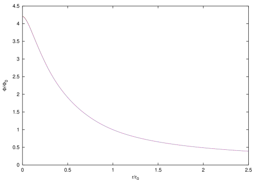
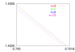
FIG. 1.: Gravitational potential $\Phi^{(n)}$ seen in the direction $\theta=\pi/2$ after $n=0$ (in red), 1 (in green), 5 (in blue) and 10 (in purple) recursions, with $r_{\rm opt}=r_{\rm max}/\pi$, $r_{0}=2r_{\rm max}/\pi$, $\theta_{0}=\pi/2$. The functions are seen to converge quickly.

In this example, the value $\Phi=\Phi_{0}$ is reached at $r=2\,r_{\rm opt}$ in the disk plane, and $r=1.85\,r_{\rm opt}$ in the orthogonal direction. The oblate form of the equipotentials is seen on figure 2.

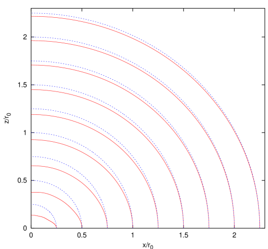
FIG. 2.: Equipotential lines generated by a disk-shaped density and a scalar field halo (in red), compared to spherical equipotentials (in blue). This plot has been computed in the case ($r_{\rm opt}=r_{\max}/\pi$ , $r_{0}=2r_{\rm max}/\pi$, $\theta_{0}=\pi/2$). The cartesian coordinate $(x,z)$ are such that the axis of revolution of the galaxy corresponds to $x=0$.

A good test of the recursive method is to pick up different values of $\theta_{0}$, and to see whether there is always a value $r_{0}(\theta_{0})$ such that: $\Phi_{0}$ is always the same, and the solutions $\Phi(r,\theta)$ are exactly identical. We checked this successfully on various examples.

The rotation curve can be deduced from the gravitational potential:

$$v^{2}=r\frac{\partial}{\partial r}\Phi(r,\theta=\pi/2)\,.$$ (48)

On figure 3, we compare the rotation curve obtained following our method with the one calculated in the approximation of Paper I: namely, replacing the thin disk by a spherical one, with a density such that in absence of any halo, the rotation curve along the stellar plane would be the same as with the true non-spherical disk. In presence of a halo, one can see that the difference becomes important only at large radius.

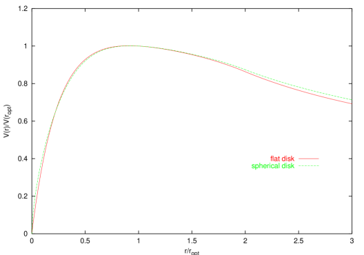
FIG. 3.: Rotation curve due to a disk-shaped density (in red) compared to that obtained in a spherical approximation (in green) as in Paper I. These two examples have been computed in the case ($r_{\rm opt}=r_{\rm max}/\pi$ , $r_{0}=2r_{\rm opt}$, $\theta_{0}=\pi/2$). The difference is seen to be fairly small.

IV The rotation curves of dwarf spirals

Dwarf spiral galaxies are known to be completely dominated by dark matter at all radii. Usual CDM models fail to reproduce the rotation curves of those systems. The purpose of this analysis is to investigate whether a self–interacting massive scalar field halo is able to reproduce such rotation curves. Therefore, we will first scrutinize the typical dwarf spiral galaxy DDO 154 that has been thoroughly studied – see for example the observations by [27] and [28]. Because it is isolated and therefore seems to be protected against any external influence, this dwarf spiral features a prototypical example for our study. Its HI gas contribution is well measured and follows the distribution

$$\rho_{\rm gas}\left(r,\theta\right)\;=\;\rho_{\rm gas}^{c}\,\exp\left\{-0.8\,|\cos\theta|\,{\displaystyle\frac{r}{r_{\rm opt}}}\right\}\,\exp\left\{-5\,|\sin\theta|\,{\displaystyle\frac{r}{r_{\rm opt}}}\right\}\;\;.$$ (49)

Its optical radius $r_{\rm opt}$ is equal to 1.4 kpc. The contribution of its stars is visible and therefore well–known, with a density distribution given by relation (45). Both stars and gas account for a small fraction of the observed circular velocity.

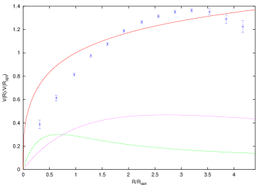
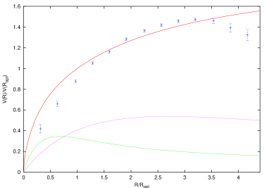
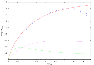
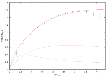
FIG. 4.: From left to right and top to bottom, the best fit of the DDO 154 rotation curve (in red) is featured as well as the observed stellar (in green) and gas (in purple) densities. A dark matter component has been added and various profiles have been assumed : Moore’s density (a), NFW profile (b), isothermal halo (c) and Burkert’s phenomenological distribution (d).

In order to compare the various dark matter models with the observations of DDO 154, we have performed a $\chi^{2}$ test on the 13 data points from ref. [28]. To commence, we have considered models in which the approximate real density of stars and gas has been assumed with $\rho_{\rm gas}^{c}\approx 0.15\,\rho_{\rm stars}^{c}$ and $v_{\rm stars}(r_{\rm opt})\approx 0.3$ – $0.4\;v_{\rm tot}(r_{\rm opt})$ – where $v_{\rm stars}$ is the stellar contribution to the rotation velocity $v_{\rm tot}$. The precise value of the ratio $v_{\rm stars}(r_{\rm opt})/v_{\rm tot}(r_{\rm opt})$ is unknown and has been adjusted here in order to provide the best fit. On top of stars and gas, a dark matter component is added with a density profile that depends on the model at stake. The Moore’s model [1] is featured in the panel (a) of fig. 4 and corresponds to the spherical symmetric density

$$\rho_{\rm M}(r)\;=\;\rho_{\rm M}^{c}\;\left\{{\displaystyle\frac{r_{\rm opt}^{3}}{r^{1.5}\,\left(r+r_{s}\right)^{1.5}}}\right\}\;\;,$$ (50)

where $r_{s}$ is a scale radius parameter that is also adjusted in the fit. Recent CDM N–body simulations point towards such a profile. In the case of DDO 154, the best fit corresponds to $\rho_{\rm M}^{c}\,\left(r_{\rm opt}/r_{s}\right)^{1.5}\approx 0.07\,\rho_{\rm stars}^{c}$ and to very large values of the scale radius $r_{s}$. The $\chi^{2}$ value is found to be approximatively equal to 600 for 10 degrees of freedom. As previously mentioned, Moore’s model where the density diverges like $r^{-1.5}$ in the central region fails to account for the dark matter distribution inside DDO 154. Then, we have tested a NFW spherical density profile [29] where

$$\rho_{\rm NFW}(r)\;=\;\rho_{\rm NFW}^{c}\;\left\{{\displaystyle\frac{r_{\rm opt}^{3}}{r\,\left(r+r_{s}\right)^{2}}}\right\}\;\;.$$ (51)

Such a distribution peaks at the center and has also been found to naturally arise in N–body numerical simulations of neutralino dark matter. We find that the best $\chi^{2}$ lies around 200 when $r_{s}\approx 9\,r_{\rm opt}$ and $\rho_{\rm NFW}^{c}\approx 6\,\rho_{\rm stars}^{c}$ – see panel (b) of fig. 4. We have also considered an isothermal spherical halo [30] with

$$\rho_{\rm iso}(r)\;=\;\rho_{\rm iso}^{c}\;\left\{{\displaystyle\frac{r_{\rm opt}^{2}}{r^{2}+r_{s}^{2}}}\right\}\;\;.$$ (52)

This density has been introduced in order to account for flat rotation curves. In the case of DDO 154 where the circular speed starts to decrease beyond 4.5 kpc, the best fit is obtained for $r_{s}\approx 1.2\,r_{\rm opt}$ and $\rho_{\rm iso}^{c}\approx 0.15\,\rho_{\rm stars}^{c}$. The corresponding $\chi^{2}$ is now far more better with a value $\sim$ 55 – see panel (c) of fig. 4. Finally, a Burkert spherical distribution [31]

$$\rho_{\rm B}(r)\;=\;\rho_{\rm B}^{c}\ \left\{{\displaystyle\frac{r_{\rm opt}^{3}}{\left(r+r_{s}\right)\,\left(r^{2}+r_{s}^{2}\right)}}\right\}\;\;,$$ (53)

has been considered. This density law has a core radius of size $r_{s}$ – just like the isothermal halo – and converges at large distances towards a Moore or a NFW profile. It has been introduced as a phenomenological explanation of the rotation curves of dwarf galaxies [32]. The best parameters are then $r_{s}\approx 1.9\,r_{\rm opt}$ and $\rho_{\rm B}^{c}\approx 6\,\rho_{\rm stars}^{c}$, leading to a best $\chi^{2}\sim 45$ – see panel (d) of fig. 4. At this stage, we reach the conclusion that neutralino dark matter – should it collapse according to the N–body numerical simulations à la Moore or NFW – is too much peaked at the center of DDO 154 and does not account for the rotation curve in that region. The fact that these species fail to reproduce the inner dynamics of a system known to be saturated by dark matter is definitely a problem. The isothermal and Burkert halos provide a better agreement with the data but are not consistent with the decrease observed beyond 4.5 kpc.

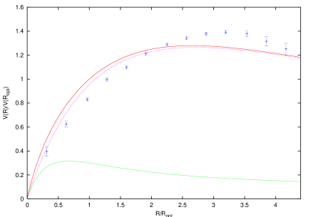
FIG. 5.: The DDO 154 rotation curve (in red) is fitted with the observed stellar density (in green) while the gas distribution (in purple) has been artificially enhanced with respect to the observed HI by a rescaling factor.

We have then investigated a slightly different idea. Following Pfenniger and Combes [33], the dark matter inside galaxies would consist of pure molecular hydrogen $H_{2}$ – so cold that it would have gone undetected so far. The formation of stars in the inner parts and its concomitant UV light production would have turned part of the $H_{2}$ into detectable HI. The distribution of this hidden $H_{2}$ component could be derived in the case of DDO 154 from its observed rotation curve. We will nevertheless adopt the opposite point of view since our aim is to derive – and not to start from – the circular speed. We have therefore artificially rescaled the observed gas density (49) by a homogeneous overall factor. The best fit featured in fig. 5 corresponds to $\rho_{\rm gas}^{c}\;=\;\rho_{\rm stars}^{c}$ and leads to a best $\chi^{2}$ of $\sim$ 500 which is not particularly exciting. In the case of the models of fig. 4, the addition of such a cold gas component does not improve the goodness of our fits.

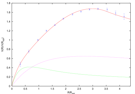
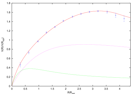
FIG. 6.: The best fit of the DDO 154 rotation curve (in red) is presented with the observed stellar density (in green) and gas distribution (in purple). In the left panel, a self–interacting bosonic halo is assumed with $m^{4}/\lambda\approx 75$ eV⁴ together with the observed gas density profile. In the right panel, the gas component has been rescaled in order to improve the goodness of fit and a value of $m^{4}/\lambda\approx 50$ eV⁴ is derived.

Finally, we have assumed the presence of a self–interacting bosonic halo and applied the recursion method discussed in section III. The left plot of fig. 6 corresponds to stellar and gas populations as observed while a value of $m^{4}/\lambda\approx 75$ eV⁴ provides a best $\chi^{2}$ of 16. The agreement with the measured rotation curve is quite good. Notice that the bosonic halo dominates completely the inner dynamics beyond $\sim$ 0.5 kpc. More impressive is the right plot of fig. 6 where the gas distribution has now been rescaled in order to improve the goodness of fit. A best $\chi^{2}$ of $\sim 7$ is reached for $\rho_{\rm gas}^{c}\approx 0.35\,\rho_{\rm stars}^{c}$ and a value of $m^{4}/\lambda\approx 50$ eV⁴.

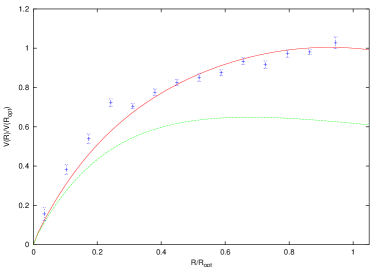
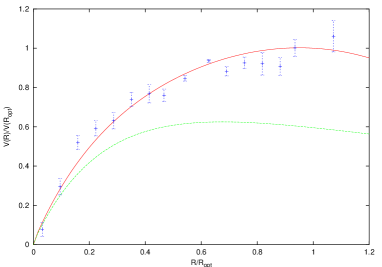
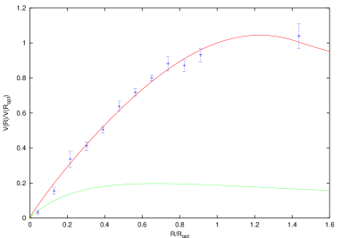
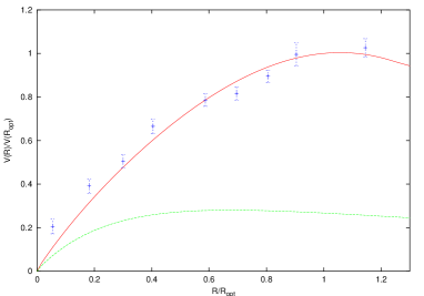
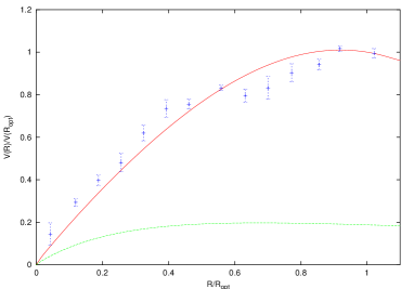
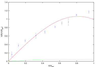
FIG. 7.: From left to right and top to bottom, the best fit (in red) of the rotation curves of various spiral galaxies with increasing optical radii. The green lines stand for the stellar contributions. The various panels respectively correspond to (a) N7339 ($r_{\rm opt}$ = 4.8 kpc) – (b) M–3–1042 ($r_{\rm opt}$ = 4.8 kpc) – (c) N755 ($r_{\rm opt}$ = 4.8 kpc) – (d) 116–G12 ($r_{\rm opt}$ = 5.4 kpc) – (e) 563–G14 ($r_{\rm opt}$ = 6.4 kpc) – (f) 545–G5 ($r_{\rm opt}$ = 7.7 kpc).

Beside the prototypical example of DDO 154, we have analyzed a set [32] of small and medium size spiral systems for which measurements of the rotation curve are of high quality. These galaxies have been selected on the requirement that they have no bulge, very little HI – if any – and a dominant stellar disk that accounts for the dynamics in the central region. They are also dominated by dark matter as is clear from fig. 7. A self–interacting bosonic halo has been assumed with $m^{4}/\lambda\approx 50$ eV⁴. Because of the presence of wiggles in the rotation curves – presumably related to spiral arms inside the disks – the best $\chi^{2}$ value becomes meaningless. The qualitative agreement is nevertheless correct except in the case of 545–G5 where the optical radius is $r_{\rm opt}$ = 7.7 kpc. Because the mass $m$ and the coupling $\lambda$ define a unique scale of $\sim$ 2.3 kpc – see relation (25) – the Bose condensate does not extend enough to account for the dark matter inside large systems. A single self–interacting bosonic halo fails to reproduce at the same time the dark matter inside light and massive spirals. A possible solution lies in the existence of several small bosonic condensates or clumps inside the halos of large galaxies whereas a single condensate would account for the dark matter of dwarf spirals such as DDO 154. We have concentrated on dwarf spiral galaxies for which neutralinos seem to be actually in trouble. The case of several bosonic clumps is beyond the scope of this work and will be investigated elsewhere.

V The solar system

As long as we were interested in the inner dynamics of galactic systems, the baryonic density $\rho_{\rm\,b}$ in equations (23) and (33) was implicitly averaged over distances of order a few pc and behaved smoothly. If the stellar population is now made of point–like particles with mass $M_{i}$, the gravitational potential $\Phi$ varies according to

$$\Delta\Phi\,+\,8\,\pi\,G\;{\displaystyle\frac{m^{4}}{\lambda}}\,\left(\Phi-\Phi_{0}\right)\,{\cal H}\left(\Phi_{0}-\Phi\right)\;=\;4\,\pi\,G\;{\displaystyle\sum_{i}}\,M_{i}\,\delta^{3}\left(\vec{r}-\vec{r_{i}}\right)\;\;.$$ (54)

Outside the Bose condensate, the usual Poisson equation is recovered so that the gravitational attraction of a star – say the Sun – is not modified with respect to the conventional situation. Slightly different is the case where the Sun lies inside the region where the field $\phi$ extends. Intuitively, the scalar field is expected to be attracted by the solar gravity and to concentrate around the Sun whose gravity should consequently be strengthened. In order to investigate that effect, we first notice that the potential difference $\Phi-\Phi_{0}$ is a linear function of the sources within the Bose condensate. The contribution $\Phi_{\odot}$ of the sun to the potential difference $\Phi-\Phi_{0}$ satisfies the modified Poisson equation

$$\Delta\Phi_{\odot}\,+\,8\,\pi\,G\;{\displaystyle\frac{m^{4}}{\lambda}}\,\Phi_{\odot}\;=\;4\,\pi\,G\;\rho_{\odot}\;\;,$$ (55)

with the condition that it must vanish on the boundaries of the Bose condensate. If the solar system is well embedded inside the latter – below a depth well in excess of a few AU – the surface of the condensate is so far that we may just require that $\Phi_{\odot}$ vanishes at infinity.

Assuming in addition that the solar density $\rho_{\odot}$ has an isotropic distribution, the solution of eq. (55) readily obtains in terms of the spherical Bessel functions $j_{0}(z)={\sin}z/z$ and $n_{0}(z)=-\,{\cos}z/z$ as explained in Appendix B

$$\Phi_{\odot}(r)\;=\;-\,4\,\pi\,G\;{\displaystyle\frac{L^{3}}{r}}\;\left\{{\cos}z\,{\displaystyle\int_{0}^{\displaystyle z}}\rho_{\odot}(u)\,u\,{\sin}u\,du\;+\;{\sin}z\,{\displaystyle\int_{\displaystyle z}^{+\infty}}\rho_{\odot}(u)\,u\,{\cos}u\,du\right\}\;\;.$$ (56)

The dimensionless radial coordinate $z$ is defined as the ratio $r/L$ where the typical scale $L$ has already been defined in section II. Relations (24) and (25) imply that $L$ exceeds the solar radius $R_{\odot}$ by some ten to eleven orders of magnitude. The gravitational potential which the Sun generates with the help of the scalar field $\phi$ simplifies into

$$\Phi_{\odot}(r)\;=\;-\,{\displaystyle\frac{G\,M_{\odot}}{r}}\,\cos\left({\displaystyle{r}/{L}}\right)\;\;.$$ (57)

Because of our assumption as regards the boundary condition – which we placed at infinity – this relation may be safely used only for distances $r\ll L$. Inside the solar system, this leads to the potential

$$\Phi_{\odot}(r)\;=\;-\,{\displaystyle\frac{G\,M_{\odot}}{r}}\,\left\{1\,-\,{\displaystyle\frac{r^{2}}{2\,L^{2}}}\right\}\;\;,$$ (58)

and to the gravitational field

$$g(r)\;=\;-\,{\displaystyle\frac{G\,M_{\odot}}{r^{2}}}\,-\,{\displaystyle\frac{G\,M_{\odot}}{2\,L^{2}}}\;\;.$$ (59)

Should the solar system be embedded inside the Bose condensate of the field under scrutiny in this article, the various planets and satellites that orbit around the Sun should undergo the additional constant radial attraction

$$\delta g\;=\;2.85\times 10^{-18}\;{\rm cm\,s^{-2}}\;\;\left\{{\displaystyle\frac{10^{-2}}{\lambda}}\right\}\;\left\{{\displaystyle\frac{m}{1\,{\rm eV}}}\right\}^{4}\;\;.$$ (60)

This acceleration is so weak that it should not alter the motion of the planets around the Sun. The relative increase of the solar gravitational attraction is actually

$${\displaystyle\frac{\delta g}{g}}\;=\;1.93\times 10^{-17}\;\;\left\{{\displaystyle\frac{r}{\rm 1\,AU}}\right\}^{2}\;\left\{{\displaystyle\frac{10^{-2}}{\lambda}}\right\}\;\left\{{\displaystyle\frac{m}{1\,{\rm eV}}}\right\}^{4}\;\;.$$ (61)

Detailed analysis of radio metric data from Pionner 10 and 11 indicate the existence of an apparent anomalous acceleration acting on these spacecrafts [34]. Quite exciting is the observation that this anomalous acceleration $\delta g_{P}$ is constant and directed towards the Sun. Both features are actually expected in the presence of a self–interacting scalar field. However, the magnitude of the observed anomalous acceleration $\delta g_{P}\sim 8.5\times 10^{-8}$ cm s^-2 is ten orders of magnitude larger than what is needed to explain the rotation curve of DDO 154. Should the Pioneer acceleration be the consequence of a scalar field enhanced solar gravity, it would indicate an exceedingly large value for $m/\lambda^{1/4}$ of order 1.3 keV and a typical condensate size $L\sim 9\times 10^{-3}$ pc. We are therefore lead to the conclusion that we cannot explain with the same value of $m/\lambda^{1/4}$ the Pioneer anomalous acceleration and the rotation curves of dwarf spirals.

VI Cosmological behavior

We will now consider briefly the possible cosmological behavior of our scalar field. In Paper II, we studied the cosmological evolution of a homogeneous complex scalar field with a quadratic and/or quartic potential. Here, we want to update this analysis for the values of $m^{4}/\lambda$ found in section IV. Generally speaking, focusing on the homogeneous quantities is the first step in any comprehensive study of a given cosmological scenario. In our case, we need to know whether the evolution of the field background violates any cosmological bound before studying the possible growth of spatial fluctuations – hoping that they will cluster and form galactic halos after the time of equality between radiation density and field density.

We refer the reader to Paper II for a detailed resolution of the Klein–Gordon and Friedman equations in a Universe containing ordinary radiation, baryons, a homogeneous complex field and a cosmological constant relevant only today. It is straightforward to show that when the potential is dominated by the quartic term, the energy density of the field smoothly decays as $a^{-4}$: so, in the early Universe, the scalar field behaves as “dark radiation”. Later, when the quadratic term takes over, i.e., when

$$m^{2}|\phi|^{2}\sim\lambda\,|\phi|^{4}\qquad\Rightarrow\qquad V(\phi)\,\sim\,2\,\frac{m^{4}}{\lambda},$$ (62)

the field starts to decay as $a^{-3}$, like dark matter: so, it can be responsible for a “matter-like” dominated stage. During the whole cosmological evolution, the kinetic energy of the field is of the same order of magnitude as its potential energy. So, the ratio $m^{4}/\lambda$ immediately gives a rough estimate of the total energy density of the field at the time of its transition, denoted later as $\rho_{\phi}^{tr}$. If this density is $\sim$ 1 eV⁴, we immediately notice that it is of the same order of magnitude as the density at radiation–matter equality – remember that $\rho_{\rm eq}\simeq 0.55$ eV⁴ for the concordance $\Lambda$CDM model. So, in the early Universe, the density of our “dark radiation” (the scalar field) had to be comparable to that of “true radiation” (photons and neutrinos). This brings some considerable tension with the bound on the total radiation density that can be derived from BBN.

This cosmological toy–model and the problems associated with it were first discussed by Peebles [17] in the case of a real scalar field, with essentially the same motivations as in the present work. As a possible way out, Peebles proposed a small modification of the scalar potential,

$$V(\phi)=m^{2}\phi^{2}+\lambda\phi^{q},$$ (63)

where $q$ would be non–integer and slightly smaller than 4. Indeed, by lowering the index $q$, one can decrease the fraction of dark radiation in the early Universe, and in particular at BBN. We will not follow this direction. Indeed, the analysis of section IV revealed a preferred value of $m^{4}/\lambda$ around 50–75 eV⁴. This is significantly larger than the observed value of $\rho_{\rm eq}$ and than the rough estimate of Paper I where we considered $m^{4}/\lambda\simeq 1$ eV⁴. Our purpose in the rest of this section will be to check whether this new value is compatible with the BBN bound.

In order to obtain a precise relation between the parameter $m^{4}/\lambda$ and the effective number of neutrinos at BBN – which is a convenient way to parameterize a cosmological density which behaves like some extra relativistic degrees of freedom – we need to study numerically the detailed behavior of the field in a vicinity of the transition between the radiation–like and the matter–like regimes. For each value of $m^{4}/\lambda$, it is possible to follow $\rho_{\phi}$, and to extrapolate the branches in $\rho_{\phi}\propto a^{-4}$ and in $\rho_{\phi}\propto a^{-3}$. We define $\rho_{\phi}^{\rm tr}$ as the energy density given by intersecting the two asymptotes. The knowledge of this single number is sufficient in order to relate exactly the constant value of $\rho_{\phi}a^{4}$ in the early Universe to the constant value of $\rho_{\phi}a^{3}$ measured today. A simple numerical simulation gives

$$\rho_{\phi}^{\rm transition}=2.4\;m^{4}/\lambda$$ (64)

independently of any other field or cosmological parameters. The simulation also provides a very good analytic approximation of the field density at any time – imposing that today, when $a=a_{0}$, the field density is given by the fraction of the critical density usually attributed to Cold Dark Matter, $\rho_{\phi}=\Omega_{\rm cdm}\rho_{c}^{0}$:

$$\rho_{\phi}=\Omega_{\rm cdm}\rho_{c}^{0}\left[(a_{0}/a)^{6}+\left(\Omega_{\rm cdm}\rho_{c}^{0}\,\frac{\lambda}{2.4\,m^{4}}\right)^{2/3}(a_{0}/a)^{8}\right]^{1/2}\;\;.$$ (65)

The field density before the transition can be read directly from the previous equation. It can be conveniently parameterized in terms of an effective neutrino number, defined as usual through

$$\Delta N_{\rm eff}=\frac{\rho_{\phi}}{\rho_{\nu}}\;\;,$$ (66)

where $\rho_{\nu}$ is the standard density of a single relativistic neutrino species. The final result is

$$\Delta N_{\rm eff}=\left(\frac{\Omega_{\rm cdm}^{4}\,\,\rho_{c}^{0\,4}\,\,\lambda}{\,\,\,\,\,2.4\,\,\,\,\,\,\rho_{\nu}^{0\,3}\,\,m^{4}}\right)^{1/3}=7.5\left(\frac{\Omega_{\rm cdm}h^{2}}{0.13}\right)^{4/3}\left(\frac{\lambda^{1/4}eV}{m}\right)^{4/3}\;\;.$$ (67)

Sticking to $m^{4}/\lambda=50~{}({\rm eV})^{4}$, and using the currently preferred values $h=0.68$ and $\Omega_{\rm cdm}=0.3$, one finds $\Delta N_{\rm eff}=2$, which is above the usual BBN bound $|\Delta N_{\rm eff}|<1$ [35]. However, it is still possible to find some values of ($\Delta N_{\rm eff}$, $h$, $\Omega_{\rm cdm}$) satisfying the above relation, and allowed at the 1–$\sigma$ level by current CMB experiments and BBN predictions [36] – for instance, (1.0, 0.63,0.20). In any case, in a very near future, the new CMB observations will set some stringent limits on these three parameters: it will then be easy to state about the validity of our alternative to the usual cosmological scenario.

VII Conclusions

We have shown that a self–coupled charged scalar field provides an excellent fit to the rotation curve of the dwarf spiral DDO 154. That galaxy is the prototypical example of a system known to be completely dominated by dark matter. The effect of the quartic coupling $\lambda$ results into an effective modified gravitation inside the Bose condensate where the Poisson equation becomes strongly non–linear. The problem – complicated by the non–sphericity of the baryon distribution – has been solved exactly as explained in section III. The agreement with the observations of the circular speed of DDO 154 is impressive. Notice that neutralino dark matter does not pass this test because of the central cusp that it would develop. We conclude that the charged scalar field considered in this analysis provides an exciting alternative to the galactic dark matter – at least inside dwarf systems. A typical value of $m^{4}/\lambda\sim$ 50 – 75 eV⁴ obtains.

The scalar field behaves cosmologically as a dark radiation component as long as the quartic contribution of the potential $V\left(\phi\right)$ dominates over its quadratic counterpart. The situation gets reversed when the field energy density is $\sim 2.4\;m^{4}/\lambda$ and a matter–like behavior subsequently ensues. The larger the crucial parameter $m^{4}/\lambda$, the sooner the transition between dark radiation and dark matter–like behaviors and consequently the smaller the contribution of the scalar field to the overall radiation density at early times – for a fixed scalar field mass density today. A large value of $m^{4}/\lambda$ translates into a small number of effective neutrino families during BBN and we have shown that our model marginally satisfies the requirement that $\Delta N_{\rm eff}$ should not exceed 1.

Actually the model is strongly constrained on the one hand side by the size $L$ of the Bose condensates – and therefore of the corresponding galactic halos – and on the other hand side by the contribution $\Delta N_{\rm eff}$ to the radiation density at BBN. Both $L$ and $\Delta N_{\rm eff}$ decrease with $m^{4}/\lambda$ and a value for the latter of $\sim$ 50 – 75 eV⁴ – which provides excellent agreement with DDO 154 – is marginally consistent with BBN. Large halos cannot consequently been pictured in terms of a single Bose condensate and the simple scheme presented here has to be modified. A possible solution – yet not very natural – is to replace the quartic field self–interaction by a $\phi^{q}$ term as suggested by [17]. This would alleviate the BBN constraint.

Another option worth being explored is to imagine that massive and extended halos are formed of several bosonic clumps. The coherent configuration that has been investigated here may be understood as the ground state of some gigantic bosonic atom. It is therefore conceivable that the scalar field may also form several such condensates that would be organized inside a huge bosonic molecule with a spatial extension much in excess of $L$. The electron cloud around the proton does not extend further than $\sim 10^{-10}$ m inside the hydrogen atom and yet electrons are delocalized over meter size distances inside metals.

If so, the dark matter would be made of small bosonic clumps. Should the solar system lie within such a system, the motion of its planets would provide in that case a lower bound on $L$ since the smaller is the latter, the stronger is the effective modification to Newton’s law of gravitation. We have actually shown in section V that the scalar field concentrates in the solar potential well and strengthens it to generate an additional gravitational attraction that is radial and constant. As a matter of fact, the radio data from the Pioneer probes are consistent with such an anomalous acceleration that seems to be constant and directed towards the Sun. Assuming that it results from the self–interacting scalar field which we have investigated in this work, the observed magnitude $\delta g_{P}\sim 8.5\times 10^{-8}$ cm s^-2 would imply a value for $m/\lambda^{1/4}$ of order 1.3 keV and a typical condensate size $L\sim$ 0.01 pc. The merging of many of these small bosonic clumps into a larger structure like a galactic halo is an open question.

A

The purpose of this section is to derive the gravitational potential generated by a pure scalar field condensate. This calculation is complementary to the one at the end of section II, based on the polytropic formalism. In absence of a baryonic density $\rho_{b}$, eq. (23) reads

$$\Delta\left(\Phi-\Phi_{0}\right)+8\pi G\frac{m^{4}}{\lambda}\left(\Phi-\Phi_{0}\right){\cal H}\left(\Phi_{0}-\Phi\right)=0\,.$$ (A1)

Since there is no source, let us suppose that the gravitational potential has a spherical symmetry. One can do a change of variable $r=z\sqrt{\frac{\lambda}{8\pi Gm^{4}}}$ so that the equation becomes simply

$$\frac{d^{2}}{dz^{2}}\left\{z\,(\Phi-\Phi_{0})\right\}+z\,(\Phi-\Phi_{0})\,\,{\cal H}\!\left(\Phi_{0}\!-\!\Phi\right)=0\,.$$ (A2)

The only solution of this equation which is continuous and derivable everywhere, and goes to zero at infinity is

$$\Phi(z)=\left\{\begin{array}[]{ll}\displaystyle\Phi_{0}+(\Phi(0)-\Phi_{0})\frac{\sin z}{z}&{\rm if}\;\;z<\pi\qquad{\rm(see~{}Paper~{}II)}\\ \\ \displaystyle\frac{\pi\Phi_{0}}{z}&{\rm otherwise.}\end{array}\right.$$ (A3)

So, the maximum extension of the scalar field halo is $\displaystyle r_{\rm max}=\pi\sqrt{\frac{\lambda}{8\pi Gm^{4}}}$. The density of the bosonic halo is

$$\rho_{\phi}=-\frac{2m^{4}}{\lambda}\left(\Phi-\Phi_{0}\right){\cal H}\left(z-\pi\right)$$ (A4)

and the total mass is

$$M=4\pi\left(\frac{\lambda}{8\pi Gm^{4}}\right)^{3/2}\int_{0}^{+\infty}\rho_{\phi}(z^{\prime}){z^{\prime}}^{2}dz^{\prime}=\frac{\pi}{G}\sqrt{\frac{\lambda}{8\pi Gm^{4}}}\left(\Phi_{0}-\Phi(0)\right)\,.$$ (A5)

On the other hand, the Gauss theorem applied to the sphere of radius $r=r_{\rm max}$ gives

$$\Phi_{0}=-\frac{GM}{r_{\rm max}}=-\frac{GM}{\pi}\sqrt{\frac{8\pi Gm^{4}}{\lambda}}$$ (A6)

so that $\Phi(0)=2\Phi_{0}$. The solution (A3) can be rewritten as

$$\Phi(z)=\left\{\begin{array}[]{ll}\displaystyle\Phi_{0}\left(1+\frac{\sin z}{z}\right)&{\rm if}\;\;z<\pi\\ \\ \displaystyle\frac{\pi\Phi_{0}}{z}&{\rm otherwise.}\end{array}\right.$$ (A7)

B

The purpose of this Appendix is to provide a prescription for the definition of $\Phi^{(0)}$ – the starting function in the recursive method. We tested this prescription on various examples, and found that $\Phi^{(0)}$ is always a fairly good approximation of the exact solution, allowing for quick convergence.

The idea is to enforce the boundary surface on which the field density $(m^{4}/\lambda)(\Phi-\Phi_{0})\,\,{\cal H}\!\left(\Phi_{0}\!-\!\Phi\right)$ vanishes to be a perfect sphere. Of course, this has to be wrong when the baryonic density is non–spherical. So, if we impose a constant boundary radius, we need to relax the fact that the value of $\Phi$ should be constant all over the boundary. In other terms, if $r$ is the radial coordinate, we replace ${\cal H}\!\left(\Phi_{0}\!-\!\Phi\right)$ by ${\cal H}\!\left(r_{0}\!-\!r\right)$, where $r_{0}$ is an arbitrary boundary radius.

If we define a dimensionless radial coordinate $z=r\sqrt{\frac{8\pi Gm^{4}}{\lambda}}$, eq. (23) becomes

$$\Delta\Phi=S(z,\theta)+\left(\Phi_{0}-\Phi\right){\cal H}\left(z_{0}-z\right).$$ (B1)

where $S=4\pi G\rho$. After a Legendre transformation, we obtain the following set of differential equations:

$$\frac{1}{z^{2}}\frac{d}{dz}\left(z^{2}\frac{d\Phi_{l}}{dz}\right)-\frac{l(l+1)}{z^{2}}\left(\Phi_{l}-\Phi_{0}\delta_{l,0}\right){\cal H}(z_{0}-z)=S_{l}(z)$$ (B2)

where $\delta_{l,0}$ is the Kronecker symbol. Each of these equations can be solved separately on the two intervals $0\leq z\leq z_{0}$ and $z_{0}\leq z\leq\infty$, using Green functions. In terms of the spherical Bessel functions $j_{l}(z)$ and $n_{l}(z)$, the solution of eq. (B1) for $z\leq z_{0}$ is

$$\Phi_{l}(z)=\Phi_{0}\delta_{l0}+n_{l}(z)\int^{z}_{0}u^{2}j_{l}(u)S_{l}(u)du+j_{l}(z)\int_{z}^{z_{0}}u^{2}n_{l}(u)S_{l}(u)du+C_{l}^{1}j_{l}(z)$$ (B3)

where $C_{l}^{1}$ is a free constant. In the same way, for $z\geq z_{0}$, the solution is

$$\Phi_{l}(z)=-\frac{1}{2l+1}z^{-(l+1)}\int_{z_{0}}^{z}u^{l+2}S_{l}(u)du-\frac{1}{2l+1}z^{l}\int_{z}^{+\infty}u^{1-l}S_{l}(u)du-C_{l}^{2}\frac{1}{2l+1}z^{-(l+1)}$$ (B4)

where $C_{l}^{2}$ is another free constant. We impose that each Legendre coefficient of the gravitational potential is derivable and continuous on the boundary $z=z_{0}$:

$$\left\{\begin{array}[]{lll}\Phi_{l}(z_{0}^{-})&=&\Phi_{l}(z_{0}^{+})\,,\\ \\ \displaystyle\frac{d}{dz}\Phi_{l}(z_{0}^{-})&=&\displaystyle\frac{d}{dz}\Phi_{l}(z_{0}^{+})\,.\end{array}\right.$$ (B5)

This defines a unique value for each constant of integration:

$$\begin{array}[]{lll}C_{l}^{1}&=&\displaystyle\frac{(I^{2}_{l}-I^{1}_{l}-\Phi_{0}\,\delta_{l,0})(l+1)+z_{0}(J^{2}_{l}-J^{1}_{l})}{(l+1)j_{l}(z_{0})+z_{0}j^{\prime}_{l}(z_{0})}\,,\\ \\ C_{l}^{2}&=&\displaystyle\frac{-z_{0}^{l+2}(2l+1)j_{l}(z_{0})(J^{2}_{l}-J^{1}_{l})+z_{0}^{l+2}(2l+1)j^{\prime}_{l}(z_{0})(I^{2}_{l}-I^{1}_{l}-\Phi_{0}\,\delta_{l,0})}{(l+1)j_{l}(z_{0})+z_{0}j^{\prime}_{l}(z_{0})}\,,\\ \end{array}$$ (B6)

where

$$\begin{array}[]{lll}I_{l}^{1}&=&\displaystyle n_{l}(z_{0})\int_{0}^{z_{0}}u^{2}j_{l}(u)S_{l}(u)du\,,\\ \\ I_{l}^{2}&=&\displaystyle-\frac{1}{2l+1}z_{0}^{l}\int_{z_{0}}^{+\infty}u^{1-l}S_{l}(u)du\,,\\ \\ J_{l}^{1}&=&\displaystyle n^{\prime}_{l}(z_{0})\int_{0}^{z_{0}}u^{2}j_{l}(u)S_{l}(u)du\,,\\ \\ J_{l}^{2}&=&\displaystyle-\frac{l}{2l+1}z_{0}^{l-1}\int_{z_{0}}^{+\infty}u^{1-l}S_{l}(u)du\,.\\ \end{array}$$ (B7)

One can then reconstruct the gravitational potential $\Phi^{(0)}$ from

$$\Phi^{(0)}(z,\theta)=\sum_{l=0}^{+\infty}P_{l}(\cos\theta)\Phi_{l}(z)\,.$$ (B8)

So far, the approximate solution $\Phi^{(0)}$ constructed in this way depends on two arbitrary numbers: first, $z_{0}$, and second, $\Phi_{0}$, which appears explicitly in the definition of $C_{0}^{1}$ and $C_{0}^{2}$. However, $z_{0}$ and $\Phi_{0}$ have to be related in some way. Indeed, if $\Phi^{(0)}$ was an exact solution, $\Phi_{0}$ would be equal by definition to $\Phi^{(0)}(z_{0},\theta)$ for any $\theta$. In our approximation scheme, $\Phi^{(0)}(z_{0},\theta)$ is not independent of $\theta$, but we can choose a particular direction $\theta_{0}$, and impose that $\Phi_{0}=\Phi^{(0)}(z_{0},\theta_{0})$. Inserting this identity in eq. (B8), and using eq. (B3), one obtains the relation

$$\Phi_{0}=\Phi^{(0)}(z_{0},\theta_{0})=\frac{z_{0}}{\tan z_{0}}\sum_{l=0}^{+\infty}P_{l}(\cos\theta_{0})\left\{n_{l}(z_{0})\int_{0}^{z_{0}}u^{2}j_{l}(u)S_{l}(u)du+K_{l}\,j_{l}(z_{0})\right\}$$ (B9)

where

$$K_{l}=\frac{(I^{2}_{l}-I^{1}_{l})(l+1)+z_{0}(J^{2}_{l}-J^{1}_{l})}{(l+1)j_{l}(z_{0})+z_{0}j^{\prime}_{l}(z_{0})}\,.$$ (B10)

In summary, the first step of our recursive method is performed in the following order:

1. we choose a value $z_{0}$ (or $r_{0}$) and an arbitrary direction $\theta_{0}$ (that will be kept for all the following iterations).

2. we solve eq. (B9) in order to find $\Phi_{0}$.

3. we compute $\Phi^{(0)}(z,\theta)$ using eqs. (B3), (B4), (B8).

The next iterations are performed in the much simpler way described in section III.

REFERENCES

- [1] B. Moore et al., MNRAS 310 (1999), 1147.
- [2] M. D. Weinberg & N. Katz, Astrophys. J. 580, 627 (2002).
- [3] J. A. Sellwood, astro-ph/0210079.
- [4] A. S. Font, J. F. Navarro, J. Stadel & T. Quinn, Astrophys. J. 563, L1 (2001).
- [5] O. Valenzuela & A. Klypin, astro-ph/0204028.
- [6] N. Dalal & C. S. Kochanek, Astrophys. J. 572, 25 (2002).
- [7] W. B. Lin, D. H. Huang, X. Zhang & R. Brandenberger, Phys. Rev. Lett. 86, 954 (2001).
- [8] D. N. Spergel & P. J. Steinhardt, Phys. Rev. Lett. 84, 3760 (2000).
- [9] R. Ruffini & S. Bonazzola, Phys. Rev. 187, 1767 (1969).
- [10] R. Friedberg, T. D. Lee, & Y. Pang, Phys. Rev. D 35, 3640 (1987).
- [11] P. Jetzer, Phys. Rep. 220, 163 (1992).
- [12] A. R. Liddle & M. S. Madsen, Int. J. Mod. Phys. D 1 (1992), 101.
- [13] W. Hu, R. Barkana, & A. Gruzinov, Phys. Rev. Lett. 85, 1158 (2000).
- [14] A. Arbey, J. Lesgourgues and P. Salati, Phys. Rev. D 64, 123528 (2001).
- [15] A. Arbey, J. Lesgourgues and P. Salati, Phys. Rev. D 65, 083514 (2002).
- [16] M. Colpi, S. L. Shapiro & I. Wasserman, Phys. Rev. Lett. 57, 2485 (1986).
- [17] P. J. E. Peebles, astro-ph/0002495.
- [18] A. Riotto & I. Tkachev, Phys. Lett. B 484, 177 (2000).
- [19] L. A. Boyle, R. R. Caldwell & M. Kamionkowski, Phys. Lett. B 545, 17 (2002).
- [20] F. E. Schunck, astro-ph/9802258.
- [21] J. Goodman, astro-ph/0003018.
- [22] F. S. Guzman, T. Matos, Class. Quant. Grav. 17, L9 (2000); F. S. Guzman, T. Matos, H. Villegas-Brena, Rev. Mex. Astron. Astrophys. 37, 63 (2001); T. Matos, F.S. Guzman, L. A. Urena-Lopez, Class. Quant. Grav. 17, 1707 (2000); T. Matos, F. S. Guzman, Annalen Phys. 9, S1 (2000); T. Matos, F. S. Guzman, D. Nunez, Phys. Rev. D 62, 061301 (2000); T. Matos, L. A. Urena-Lopez, Class. Quant. Grav. 17, L75 (2000); Phys. Rev. D 63, 063506 (2001); M. Alcubierre, F. S. Guzman, T. Matos, D. Nunez, L. Arturo Urena-Lopez, P. Wiederhold, Class. Quant. Grav. 19, 5017 (2002).
- [23] U. Nucamendi, M. Salgado, D. Sudarsky, Phys. Rev. D 63, 125016 (2001).
- [24] C. Wetterich, Phys. Lett. B 522, 5 (2001).
- [25] L. A. Urena-Lopez, A. R. Liddle, Phys. Rev. D 66, 083005 (2002).
- [26] V. Sahni, L. Wang, Phys. Rev. D 62, 103517 (2000); F. Perrotta, C. Baccigalupi, Phys. Rev. D 65, 123505 (2002); M. Pietroni, hep-ph/0203085; J. E. Kim, H. P. Nilles, Phys. Lett. B 553 1 (2003); M. C. Bento, O. Bertolami, A. A. Sen, astro-ph/0210468; D. Carturan, F. Finelli, astro-ph/0211626; B. A. Bassett, M. Kunz, D. Parkinson, C. Ungarelli, astro-ph/0211303.
- [27] G. L. Hoffman, E. E. Salpeter and N. J. Carle, astro-ph/0107484.
- [28] C. Carignan and C. Purton, Astrophys. J. 506, 125 (1998).
- [29] J. F. Navarro, C. S. Frenk and S. D. M. White, Astrophys. J. 462, 563 (1996).
- [30] C. Caraignan and S. Beaulieu, Astrophys. J. 347, 760 (1989).
- [31] A. Burkert, Astrophys. J. 447, L25 (1995).
- [32] A. Borriello and P. Salucci, Mon. Not. Roy. Astr. Soc. 323, 285 (2001).
- [33] D. Pfenniger, F. Combes and L. Martinet, Astron. & Astrophys. 285, 79 (1994).
- [34] J. D. Anderson, P. A. Laing, E. L. Lau, A. S. Liu, M. M. Nieto, & S. G. Turyshev, Phys. Rev. Lett. 81, 2858 (1998)
- [35] S. Burles and D. Tytler, Astrophys. J. 499, 699 (1998); Astrophys. J. 507, 732 (1998).
- [36] A. Benoit et al., astro-ph/0210306.
A