The DDO IVC Distance Project: Survey Description and the Distance to $\mathrm{G}139.6+47.6$

Abstract

We present a detailed analysis of the distance determination for one Intermediate Velocity Cloud (IVC $\mathrm{G}139.6+47.6$) from the ongoing DDO IVC Distance Project. Stars along the line of sight to $\mathrm{G}139.6+47.6$ are examined for the presence of sodium absorption attributable to the cloud, and the distance bracket is established by astrometric and spectroscopic parallax measurements of demonstrated foreground and background stars. We detail our strategy regarding target selection, observational setup, and analysis of the data, including a discussion of wavelength calibration and sky subtraction uncertainties. We find a distance estimate of $129\pm 10$ pc for the lower limit and $257^{+211}_{-33}$ for the upper limit. Given the high number of stars showing absorption due to this IVC, we also discuss the small-scale covering factor of the cloud and the likely significance of non-detections for subsequent observations of this and other similar IVC’s. Distance measurements of the remaining targets in the DDO IVC project will be detailed in a companion paper.

1 INTRODUCTION

As with many objects in the Universe, Intermediate Velocity Clouds (IVC’s) are poorly understood due to a lack of distance estimates. Many of the interesting physical properties of the IVC’s (mass, density, volume, etc.) depend on the distance, and without these properties it is difficult to constrain models concerning their origins, evolution, or relative importance to the interstellar medium (Wakker & van Woerden, 1997).

There are several ways to determine the distances to IVC’s, which have been used to varying degrees of success (see Gladders et al., 1998, and references therein). One of these methods stands out as particularly successful in determining both upper and lower limits on the distances to the clouds: the absorption line method. In this method, stars along the line of sight to the cloud are used as distance markers. If a star is behind the cloud, one hopes that metallic lines at the cloud’s systemic velocity can be detected in the star’s spectrum. By determining whether stars are behind the cloud, we set upper and lower limits on its distance. Astrometric or spectroscopic parallax can then be used to determine the distances to the observed stars to bracket the cloud’s distance. Such a technique, unfortunately, requires a large investment of telescope time (Wakker & van Woerden, 1997).

We began the DDO IVC Distance Project in the summer of 1997 in the hopes that a reliable distance to the Draco cloud could be determined (see Gladders et al., 1998). The success of this project soon led to distance determinations for other IVCs (see Clarke et al., 1999). In this paper, we use the cloud $\mathrm{G}139.6+47.6$ as a case study in order to present our methodology as a precursor to the publication of the entire data set, forthcoming in a companion paper. This cloud’s Local Standard of Rest velocity is $v_{\rm LSR}=-12\ \mathrm{km}\ \mathrm{s}^{-1}$ and is one of the lowest in our sample, which range from $3.5\ \mathrm{km}\ \mathrm{s}^{-1}$ to $-47\ \mathrm{km}\ \mathrm{s}^{-1}$. Traditionally, IVC’s are distinguished by $\left|v_{\rm LSR}\right|<90\ \mathrm{km}\ \mathrm{s}^{-1}$ and $\mathrm{G}139.6+47.6$, having a relatively low velocity, might be more appropriately labeled a Low Velocity Cloud (LVC). However, as we are not discussing the origins or kinematics of these clouds, we will not make this distinction here.

2 OBSERVATIONS

2.1 Target Selection

We have taken our target list of clouds from the sample of Heiles, Reach, & Koo (1988). Among the 26 clouds, we selected 16 to observe that are at high galactic latitudes and are observable from the David Dunlap Observatory. Several of these clouds have been grouped together in pairs, as they do not seem to be separated either in angular or velocity space. We are thus left with a sample of 11 cloud complexes.

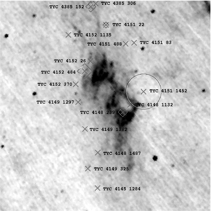
Figure 1: Positions of our target stars with respect to the IVC cloud $\mathrm{G}139.6+47.6$. A circle around a cross denotes a foreground star whereas a box around a cross denotes a background star. Both boxes and circles are drawn with an angular size inversely proportional to their nominal distances. The background gray-scale is from the IRAS $100\mu$ survey.

With the clouds selected, we then require good stellar targets along their lines of sight. We consider a “good” target to be a star with $B-V<0.35$, as we want early-type stars with as few stellar features as possible so that absorption features can be easily identified as originating in the cloud rather than the stellar photosphere. We use the Tycho Catalogue (Hoeg et al., 1997) and the USNO Catalog (Urban et al., 1998) to select our targets. Cloud sizes are estimated through both the H I atlas of Hartmann & Burton (1997) and through IRAS 100 $\mu$ maps (see Figure 1). We then search the Tycho Catalogue, using the online tools, for stars with positions within the cloud and with the appropriate colors. When the positions of the stars have been determined, we build an H I column density profile in velocity space at the position of each star (see Figure 2). Assuming hydrogen or IRAS emission is a good indication of sodium absorption (the validity of this will be discussed in §4.2), we can then determine which stars represent good probes of the cloud. Also, using the $B-V$ color index, the stars’ distances can be estimated, which further helps in target selection. Figure 1 shows the IRAS 100 $\mu$ emission for the IVC cloud $\mathrm{G}139.6+47.6$ as well as the positions of the 16 target stars that satisfied the above criteria.

2.2 Observational Setup

Since the beginning of this project, we have been assigned a total of 137 nights, of which 63 have produced useful spectra for at least a portion of the night. To date we have observed 86 stars along lines of sight to eleven different IVC’s.

Nominally, each target star is observed using two observational setups: a sodium setup and a classification setup. Both use the David Dunlap Observatory (DDO) 1.88 m telescope and Cassegrain spectrograph. The classification setup is used to classify each star so that its distance can be determined. The sodium setup is used to observe the Na I doublet to determine whether the star is behind the cloud or not. The sodium setup is at higher resolution than the classification setup, and so it represents the bulk of the observations. In addition to our program stars, spectroscopic standards are observed in both the sodium and classification setups. We observe standards in the sodium setup in order to generate template spectra for use with the cross-correlation techniques, which are detailed in §4.1.

2.2.1 Sodium Setup

The sodium setup yields a wavelength coverage of approximately 5800–6000 Å with a resolution of $0.43$ Å. With this setup, we cannot resolve any sodium absorption caused by the cloud (our velocity resolution is $22\ \mathrm{km}\ \mathrm{s}^{-1}$ at the Na I doublet); however, this is not necessary for our purposes (see §4.1). We observe targets down to a magnitude of 12.5, for which it takes 4 hours to achieve a signal to noise ratio of 50. The wavelength region of interest is significantly affected by water vapor absorption lines, so the observation of telluric standards is important. Typically, we observe three to four telluric standards throughout the night. These standards are later used to subtract the telluric lines from the sodium spectra.

2.2.2 Classification Setup

For the classification setup, we cover the range 3800–4400 Å at a resolution of $2.5$ Å. We obtain classification spectra of any stars which show definite absorption or lack of absorption by the cloud and that do not have Hipparcos distance measurements. Classification spectra of standards taken from Garcia (1989) are also obtained, covering spectral types B0 to G5 and luminosity classes I to V. These standards are used to determine the distances to several program stars using spectroscopic parallax.

3 DATA ANALYSIS

The bulk of the data reduction is now done through a processing pipeline developed using standard IRAF tasks. This pipeline allows us to quickly reduce a night’s data and also ensures a consistent procedure for all data. The rapid turnaround allows greater precision in subsequent target selection. Further, with over 20 observers working on the same project, a centralized repository of data is necessary. Such a database, implemented in HTML, was devised and became an invaluable resource.

The data are de-biased and flat-fielded using standard methods. Each two-dimensional spectrum is then rectified to a common wavelength scale. With the DDO’s close proximity to one of North America’s largest urban centers, one must be very careful in the subtraction of the sodium sky lines. Even though most of the light from high-pressure sodium lights is self-absorbed, the two sodium lines from low pressure lamps are quite bright (see Figure 3). Great care is taken to ensure proper rectification of the 2-D spectra and hence proper sky line subtraction.

Lastly, we remove the telluric lines using the spectrum of the telluric standard that is observed the closest in time to the program star. This is done by normalizing the reduced, continuum-subtracted 1-D telluric spectrum and then correcting for the difference in airmass. Figure 4 shows a typical spectrum of the telluric standard $\mathrm{HD}177724$. Two telluric standard stars were chosen due to their lack of contaminating inter-stellar features in the wavelength region of interest: $\mathrm{HD}177724$ (A0Vn, $m_{\rm V}=2.988$) and $\mathrm{HD}120315$ (B3V, $m_{\rm V}=1.852$). In order to sample the slit effectively without saturating the CCD, neutral density filters were used.

In order to test for the wavelength calibration stability, the sky lines are extracted from the dispersion-corrected 2-D spectra of every program star. Using the same cross-correlation techniques outlined in §4.1, the shift in the sky Na I emission lines is computed. The average shift is $0.35~{}\mathrm{km}\ \mathrm{s}^{-1}$ with a standard deviation of approximately $1~{}\mathrm{km}\ \mathrm{s}^{-1}$, which is consistent with no systematic shift and demonstrates the stability of the wavelength calibration.

4 DISTANCE DETERMINATION

There are three steps to the determination of a cloud’s distance: 1) testing for non-stellar contribution in Na I absorption lines, 2) assigning each star to the background or foreground, and 3) computing the distance to each star. Each of these steps is described in detail below.

4.1 Detection of Absorption by the Cloud

The most important step in the determination of a cloud distance is the detection (or non-detection) of Na I from the cloud in the spectrum of stars along the line of sight. Ideally, one would like to use early-type stars to minimize the number of stellar lines in the vicinity of the Na I doublet, and one would like to resolve the absorption due to the cloud. However, to maximize the number of target stars for this project, we have chosen later-type stars and lower resolution than other authors (Benjamin et al., 1996). Because moderate dispersion allows for a larger sampling of the underlying stellar spectrum, we can use cross-correlation techniques to decouple absorption due to the stellar envelope and any possible absorption due to the IVC. The technique is as follows.

For each star in our sample, we estimate the spectral class using the sodium part of the spectrum, or the classification spectrum if this has been obtained already. Based on this classification, we build a template sodium spectrum by measuring the central wavelength and equivalent width of all significant lines in the sodium spectrum of a standard star with similar spectral class. The template spectrum is composed of a flat continuum with absorption lines at the same wavelengths and with the same equivalent widths (though with FWHM less than the resolution of the real spectra) as would be measured at rest ($v_{r}=0$). Using the IRAF task rvcorrect, each program star’s spectrum is corrected to remove the velocity of the Earth and of the Sun relative to the Local Standard of Rest (LSR). Measurement of the Doppler shift in the absorption features relative to their rest wavelengths will therefore yield the LSR velocity of the star.

Once the template spectrum has been produced, we cross-correlate it with the spectrum of the program star in two separate regions. The first region, which we shall term the stellar region, is the whole sodium spectrum but excluding the region around the Na I doublet. The second region we shall term the sodium region, which contains only the sodium doublet. The cross-correlation of the stellar region with the template spectrum gives us an estimate of the radial velocity and the average width of the stellar features. The cross-correlation of the sodium region with the template spectrum gives us an estimate of the velocity and average width of both the stellar features and the interstellar features if both are present in the region. By comparing the cross-correlations, one can determine whether or not there are any Na I features due to interstellar absorption and, therefore, whether the star is behind the cloud. If the stellar features are too narrow and too close to the velocity of the IVC, the star is rejected. Figure 5 shows the cross-correlations for the 4 program stars we have identified as background stars. The left panels show the Na I region of the spectra and the right panels show the cross-correlations with the template spectra.

We consider a star to have a sodium detection if the cross-correlation of the Na I D lines peaks near the velocity of the cloud and either there are no significant stellar lines or any stellar lines are at a significantly different velocity than that of the cloud. There are cases where the velocity of the stellar lines is too close to the velocity of the cloud, yet the cross-correlation peak of the stellar lines is significantly broader than that of the sodium lines, which is suggestive of absorption due to the cloud. In these cases, we label the stars as possible detections. Likewise, there are cases where the sodium and stellar lines have identical cross-correlation profiles near the velocity of the cloud and we label these as possible non-detections (see Table 1).

4.2 Detection vs. Non-detection

While the detection of absorption features due to the cloud in the spectrum of a star is strong evidence that the star is behind the cloud, the reverse is not necessarily true. A non-detection for a star can either mean the star is in the foreground, or it can simply mean the star is behind the cloud but the column density of Na I is not sufficient to produce detectable features in its spectrum. Two uncertainties arise at this point. The first is the covering factor of the cloud on small angular scales. The H I column density is sampled from a relatively large beam, whereas our stars sample sodium absorption on an extremely small angular scale. It is therefore possible that small-scale variations in the covering factor are unresolved by the large H I beam. The second uncertainty is the actual abundance of Na I relative to H I. In the absence of any Na I absorption, the ratio of Na I/H I is uncertain and could be very low. Therefore, clouds with no detections may very well have low Na I/H I. This problem could be resolved by extrapolation from other cloud metallicities, once they are determined to some degree of accuracy. An example of low Na I/H I could be $\mathrm{G}86.5+59.6$, which has eluded all our attempts at detecting Na I absorption. Our current lower limit to the distance to the cloud is 430 pc (Clarke et al., 1999). However, its rather large radial velocity of $-39~{}\mathrm{km}\ \mathrm{s}^{-1}$ may imply a large distance based on the terminal drag model of Benjamin et al. (1996), which predicts a linear correlation between the velocity perpendicular to the galactic plane and height above the plane.

Recent measurements of IVC sight-lines have shown that Na I/H I varies on the order of 70 per cent over 30 arcsec and by as much as a factor of 2 over 1 arcmin (Smoker et al., 2002). Given the large angular distances between our target stars, we cannot expect the Na I/H I ratios obtained from our detections to be constant, nor can we use them to accurately predict the expected equivalent widths of Na I in other targets. This makes the identification of foreground stars more uncertain. Nevertheless, when evaluating the significance of a non-detection, the lowest observed EW(Na I)/$\rm N_{HI}$ for the cloud is used to predict the sodium absorption one would expect if the star were behind the cloud. If this absorption is detectable by our instruments yet is not observed, we conclude the star is in the foreground. Figure 6 shows the expected sodium absorption in the spectrum of $\mathrm{TYC}\ 4151\ 1452$ if the star were behind the cloud. The 4 spectra were computed using the EW(Na I)/$\rm N_{HI}$ obtained from our 4 detections.

To address the issue of covering factor, we examine the distance distribution of our target stars. Of the 16 program stars, 4 have definite detections of Na I absorption. By obtaining distances to all these stars, one can now start to answer the question of covering factor, at least for this particular cloud complex. We wish to determine the probability that a background star will show sodium absorption due to the cloud given the H I column density along its line of sight. This can be determined in the following way. We first determine the best upper limit on the distance to the cloud (i.e., the closest star with a detection). We then look for any stars which could be farther away and count the number of detections versus the number of non-detections. If we find a non-detection which is farther away than a detection, this implies a covering factor less than unity.

If we leave out the stars for which the detections and non-detections are of low confidence, then there are 4 stars with detections behind the nominal position of the cloud and one non-detection in front. If we include the possible detections and non-detections, then there are 7 detections behind the furthest non-detection and two non-detections in front of the closest detection. In both cases, this is consistent with a covering factor of unity.

4.3 Stellar Distance Determination

For the determination of the stellar distances, we use either trigonometric parallax from Hipparcos or spectroscopic parallax using spectroscopic classification obtained either in the literature or from our own observations. Clearly, the faintest and farthest stars require spectroscopic classifications to obtain accurate distances. However, since the goal is to determine the best distance to any given H I cloud, we are more concerned with accurately determining the distance to those stars that are closest to the cloud.

To determine distances based on the spectral type of the star, we use the the spectral class and absolute magnitude calibration of Corbally & Garrison (1984) to assign an absolute magnitude to each classified star. The Tycho apparent magnitude is then used to compute the distance modulus. No correction for interstellar absorption is made as it is negligible at this galactic latitude and longitude, being near the Lockman Hole. We also ignore any extinction that may be caused by the cloud itself, as this is likely small (Stark, Kalberla, & Guesten, 1997) and can only reduce the distance of the background stars, thereby improving our distance estimates. In assigning uncertainties to our distance estimates, two factors contribute the most: the uncertainty in the classification of the spectra and the intrinsic scatter in the absolute magnitude versus spectral type relation. For the former, we assume an uncertainty of plus or minus one spectral class. For the latter, we take $\pm 0.7\ \mathrm{mag}$ (Jaschek & Gómez, 1996). For the F-type stars, there is also a larger uncertainty in establishing the luminosity class, which translates to a very large distance uncertainty. In these cases, we give distance ranges rather than uncertainties.

5 RESULTS AND CONCLUSIONS

Of the original 20 program stars, 4 were discarded due to strong stellar features at the velocity of the cloud. Seven stars were inconclusive and require higher SNR and/or higher spectral resolution than DDO can provide in order to make use of them. Table 1 lists the remaining 9 stars by Tycho name, the apparent magnitude, spectral type, distance, equivalent width, H I column density due to the cloud, and note regarding detection.

The DDO IVC Distance Project has been a resounding success and has far exceeded our initial expectations. In particular the IVC $\mathrm{G}139.6+47.6$ had a relatively large number of background stars and few foreground stars. We determine the cloud’s lower distance limit to be $129\pm 10$ pc, corresponding to the distance to $\mathrm{TYC}\ 4151\ 1452$. Our closest detection star is $\mathrm{TYC}\ 4152\ 484$, which has spectral class F5V, yielding an upper limit of $257^{+211}_{-30}$ pc.

Under the assumption that these distances are correct and given that every star behind the cloud shows a detection, we conclude that the covering factor is consistent with unity for this cloud.

To improve the distance determination, we would require more foreground stars that are more distant, as well as background stars that are closer than what is currently in our sample. We have exhausted the Tycho and USNO catalogs of appropriate stars. It is possible (though unlikely) that more candidates could be found by making a photometric survey of the region. By considering stars bluer than $B-V=0.35$, the survey would have to be complete to apparent magnitudes of $m_{\rm V}=10-11$ to sample the appropriate distances, assuming no extinction. The Tycho Catalogue is 99% complete down to $m_{\rm V}=11$ (Hoeg et al., 1997) so it is unlikely that we have missed candidate stars with spectral type earlier than F.

The distance estimate might also be improved by further study of the inconclusive stellar candidates. In particular, better modeling of the stellar features in the template spectra used for the cross-correlations could reduce ambiguity and allow one to classify a detection or non-detection with more confidence.

Figure 2: H I emission along the line of sight to the four stars with detections and the one star with no detection ($\mathrm{TYC}\ 4151\ 1452$). The velocities of the detected absorption are plotted as error bars with line styles that match their stars’ profiles.

Figure 3: Intensity of the sky at the DDO, averaged over one month. Note the self-absorption due to the high pressure sodium lights as well as the lines due to the low pressure lights.

Figure 4: Sample spectrum of the telluric standard $\mathrm{HD}177724$.

Figure 5: Na I spectra and cross-correlations for the four stars with detections. Two cross-correlations are plotted for each star: the sodium region, where only the Na I lines are used (solid line) and the stellar region, where all lines but the Na I are used (dotted line). The cloud velocities are over-plotted on the cross-correlations as error bars.

Figure 6: Expected Na I absorption in the spectrum of $\mathrm{TYC}\ 4151\ 1452$ if it were behind the cloud. The top-most spectrum is the observed spectrum. Each subsequent spectrum is labeled with the EW(Na I)/$\rm N_{HI}$ used to predict the equivalent width one would observe, which is shown in parentheses.

Table 1: List of Program Stars.

Tycho ID	$V$	MK Class	D	EW($\mathrm{D}_{1}$)	$\mathrm{N}_{HI}$	Notes
	(mag)		(parsecs)	EW($\mathrm{D}_{2}$)	($\times 10^{19}\mathrm{cm}^{-2}$)
				(mÅ)
TYC 4152 484	10.45	F5V	$257^{+211}_{-30}$	$150\pm 20$	10	detection
				$130\pm 20$
TYC 4385 152	9.66	A0V	$649^{+206}_{-157}$	$210\pm 20$	26	detection
				$200\pm 20$
TYC 4148 239	10.91	A1V	$875_{-77}^{+449}$	$310\pm 40$	57	detection
				$370\pm 40$
TYC 4151 22	10.53	A0V	$968_{-233}^{+308}$	$240\pm 40$	28	detection
				$270\pm 40$
TYC 4152 370	10.27	F0V	$342_{-58}^{+176}$	$380\pm 50$	26	possible detection
				$380\pm 50$
TYC 4145 1284	10.45	F2(IV?)	$512^{+421}_{-207}$	$330\pm 70$	37	possible detection
				$320\pm 70$
TYC 4149 325	9.8	F2(?)	$229-3000$	$260\pm 50$	14	possible detection
				$250\pm 50$
TYC 4148 1132	8.58	$\ldots$	$165\pm 25$	$\ldots$	47	possible non-detection
				$\ldots$
TYC 4151 1452	6.40	$\ldots$	$129\pm 10$	$\ldots$	19	non-detection
				$\ldots$

Note. — EW($\mathrm{D}_{1}$) and EW($\mathrm{D}_{2}$) are the equivalent widths measured using the Na I $\mathrm{D}_{1}$ and $\mathrm{D}_{2}$ lines, respectively.

References

- Benjamin et al. (1996) Benjamin, R. A., Venn, K. A., Hiltgen, D. D., & Sneden, C. 1996, ApJ, 464, 836
- Corbally & Garrison (1984) Corbally, C. J., & Garrison, R. F. 1984, in The MK Process and Stellar Classification, ed. R. F. Garrison (David Dunlap Observatory, Toronto, Canada), 277
- Clarke et al. (1999) Clarke, T. E., Mallén-Ornelas, G., Sawicki, M., Brodwin, M., McNaughton, R., Gladders, M. D., Burns, C. R., & Attard, A. 1999, in ASP Conf. Ser. 168: New Perspectives on the Interstellar Medium, 323
- Garcia (1989) Garcia, B. 1989, Bulletin d’Information du Centre de Donnees Stellaires, 36, 27
- Gladders et al. (1998) Gladders, M. D., et al. 1998, ApJ, 507, L161
- Hartmann & Burton (1997) Hartmann, D., & Burton, W. B. 1997, Atlas of galactic neutral hydrogen (Cambridge; New York: Cambridge University Press)
- Heiles, Reach, & Koo (1988) Heiles, C., Reach, W. T., & Koo, B. 1988, ApJ, 332, 313
- Hoeg et al. (1997) Hoeg, E., et al. 1997, A&A, 323, L57
- Jaschek & Gómez (1996) Jaschek, C., & Gómez, A. E. 1996, A&A, 323, 619
- Smoker et al. (2002) Smoker, J. V., Keenan, F. P., Lehner, N., & Trundle, C. 2002, A&A, 387, 1057.
- Stark, Kalberla, & Guesten (1997) Stark, R., Kalberla, P., & Guesten, R. 1997, A&A, 317, 907
- Urban et al. (1998) Urban, S. E., Corbin, T. E., Wycoff, G. L., Martin, J. C., Jackson, E. S., Zacharias, M. I., & Hall, D. M. 1998, AJ, 115, 1212
- Wakker & van Woerden (1997) Wakker, B. P., & van Woerden, H. 1997, ARA&A, 53, 217