Digital Deblurring of CMB Maps:
Performance and Efficient Implementation

Digital deblurring of images is an important problem that arises in multifrequency observations of the Cosmic Microwave Background (CMB) where, because of the width of the point spread functions (PSF), maps at different frequencies suffer a different loss of spatial resolution. Deblurring is useful for various reasons: first, it helps to restore high frequency components lost through the smoothing effect of the instrument’s PSF; second, emissions at various frequencies observed with different resolutions can be better studied on a comparable resolution; third, some map-based component separation algorithms require maps with similar level of degradation. Because of computational efficiency, deblurring is usually done in the frequency domain. But this approach has some limitations as it requires spatial invariance of the PSF, stationarity of the noise, and is not flexible in the selection of more appropriate boundary conditions. Deblurring in real space is more flexible but usually not used because of its high computational cost. In this paper (the first in a series on the subject) we present new algorithms that allow the use of real space deblurring techniques even for very large images. In particular, we consider the use of Tikhonov deblurring of noisy maps with applications to PLANCK. We provide details for efficient implementations of the algorithms. Their performance is tested on Gaussian and non-Gaussian simulated CMB maps, and PSFs with both circular and elliptical symmetry. Matlab code is made available.

1 Introduction

During the last decade, observations of the Cosmic Microwave Background (CMB) anisotropies have progressed significantly. After the first evidence of CMB intensity fluctuations measured by the COBE satellite (see Smoot 1999, and references therein), several balloon-borne and ground based experiments have successfully detected CMB anisotropies at degree and sub-degree angular scales (de Bernardis et al. 2002; Halverson et al. 2002; Lee et al. 2001; Padin et al. 2001). The MAP satellite currently in operation will soon provide full sky maps of CMB anisotropies at about $20$ arcmin. resolution and a sensitivity of the order of 10 $\mu$K, on a frequency range extending from $22$ to $90\leavevmode\nobreak\ {\rm GHz}$. This extraordinary experimental enterprise will be followed by the PLANCK satellite, scheduled for launch in 2007 , that will provide full sky maps of total intensity and polarization of CMB anisotropy at a few arcmin. resolution, and a sensitivity of a few $\mu$K, on nine frequency channels ranging from $30$ to $857\leavevmode\nobreak\ {\rm GHz}$.

These new sets of observations will pose new and challenging questions in data analysis. Methods will have to be developed to process the large amount of incoming data, and to extract and separate cosmological information from foreground emissions from extra-Galactic sources as well as from our own Galaxy.

An important question is the creation of sky maps based on small angular scale time ordered data from all-sky CMB observations of MAP and PLANCK; efficient map-making algorithms based on a maximum likelihood approach have been proposed (Natoli et al. 2001; Borrill et al. 2001; Stompor et al. 2002). Regarding the separation of emissions coming from different astrophysical processes, multifrequency observations can be exploited. For example, available prior information about the signals can be used in a regularised inversion via Wiener filtering and maximum entropy methods, either on small sky patches (Hobson et al. 1998) or on the whole sky (Bouchet & Gispert 1999; Stolyarov et al. 2002). It has been shown that under certain independence assumption on the signals, the map-operating algorithms based on Independent Component Analysis (ICA) techniques can be applied on sky patches (Baccigalupi et al. 2000) as well as on the whole sky (Maino et al. 2002).

In this paper we study a different problem. We consider the effects of the beam of the instrument used to gather the observations. We present efficient numerical methods to estimate the emission pattern lost through the degradation of the instrument’s point spread function (PSF) and noise contamination. This “deblurring” process may prove very useful in CMB data analyses: first, it helps recover high frequencies smoothed out by the instrument’s PSF. Second, a better understanding of sky emissions, from foregrounds in particular, is achieved if multifrequency sky maps are compared on a common resolution. Third, some map-based component separation algorithms, such as ICA (Baccigalupi et al. 2000; Maino et al. 2002) require input maps with similar level of degradation. Furthermore, although the aim of satellite missions such as Planck and MAP is to obtain full sky maps of the CMB, the strength of the CMB over other backgrounds or contaminating sources will vary over the sky. Therefore, even if some characteristics of CMB are estimated on full sky maps, it will be convenient to check these results on smaller sky patches where CMB dominates the other components (e.g., at high Galactic latitude and at high observing frequency) and data are free from instrumental and/or observational problems.

Most deblurring of CMB data has been done in frequency space, (see Hobson et al. 1998; Stolyarov et al. 2002). This approach is computationally efficient but has some important limitations; it requires the stationarity of the contaminating noise and the spatial invariance of the PSF. Furthermore, it implicitly assumes periodic boundary conditions which, as we show below, is not necessarily the best choice. Tikhonov regularization provides a more flexible real domain deblurring technique that can be used when any of these assumptions are not met.

Until recently, Tikhonov deblurring was avoided because of its computational cost. For example, for an $N\times N$ pixel image in the frequency domain one works with $N\times N$ matrices, while in the spatial domain the matrices are of dimension $N^{2}\times N^{2}$. However, new efficient algorithms that overcome this problem have made Tikhonov deblurring a competitive alternative to frequency domain techniques. In this first paper, we present some of these algorithms and show their good performance not only in regards to their computational cost but also in regards to their numerical stability, which is an important characteristics in any ill-posed inversion problem. Furthermore, we will present some preliminary results concerning the deblurring for the case of spatially varying PSFs. A detailed treatment of this problem will be provided in a future paper.

The rest of the paper is organized as follows. In Sects. 2 and 3 we provide a formal definition of the map-based deblurring process, focusing on boundary conditions and numerical issues. In Sect. 4 we discuss a regularization approach that is efficient and flexible for deblurring noisy maps; results of numerical experiments are provided in Sect. 5. Our first application to a realistic map is presented in Sect. 6, where we consider a region in the sky (already addressed by Baccigalupi et al. 2000) in which the CMB emission largely dominates over foregrounds. We will assume observational conditions, frequencies, angular resolution and noise level corresponding to the Low Frequency Instrument (LFI) of the PLANCK satellite. Further simulations are presented in Sects. 7 and 8 where we consider non-Gaussian random fields and spatially varying PSFs. In Sect. 9 we close with final comments and conclusions.

2 Formalization of the problem

When a two-dimensional object $f(\xi,\eta)$ is observed through an optical (linear) system, it is seen as an image $g(x,y)$

$$g(x,y)=\int\limits_{-\infty}^{+\infty}\int\limits_{-\infty}^{+\infty}h(x,y,\xi,\eta)f(\xi,\eta)\leavevmode\nobreak\ d\xi\leavevmode\nobreak\ d\eta,$$ (1)

where the function $h(x,y,\xi,\eta)$, called a point-spread function (PSF), represents the blurring action of the optical instrument. Model (1) allows the PSF to vary with position in both $(x,y)$ and $(\xi,\eta)$ variables (space-variant PSF). Often, it is possible to simplify this model by assuming that the PSF is independent of position (space-invariant PSF), and thus

$$g(x,y)=\int\limits_{-\infty}^{+\infty}\int\limits_{-\infty}^{+\infty}h(x-\xi,y-\eta)f(\xi,\eta)\leavevmode\nobreak\ d\xi\leavevmode\nobreak\ d\eta.$$ (2)

Another useful simplification occurs when PSF is separable, which means that it can be written in the form

$$h(x,y,\xi,\eta)=h_{1}(x,\xi)\leavevmode\nobreak\ h_{2}(y,\eta),$$ (3)

for the space-variant PSF, and

$$h(x-\xi,y-\eta)=h_{1}(x-\xi)\leavevmode\nobreak\ h_{2}(y-\eta),$$ (4)

for the space-invariant PSF. In this case models (1), (2) can be simplified to

$$g(x,y)=\int\limits_{-\infty}^{+\infty}h_{1}(x,\xi)\left[\int\limits_{-\infty}^{+\infty}h_{2}(y,\eta)f(\xi,\eta)\leavevmode\nobreak\ d\eta\right]d\xi,$$ (5)

and

$$g(x,y)=\int\limits_{-\infty}^{+\infty}h_{1}(x-\xi)\left[\int\limits_{-\infty}^{+\infty}h_{2}(y-\eta)f(\xi,\eta)\leavevmode\nobreak\ d\eta\right]d\xi,$$ (6)

respectively. We see that separability of the PSF implies independent blurring along the horizontal and vertical directions.

Models (1), (2), (5), and (6) are only theoretical. In practical applications, we only have discrete noisy observations of the image $g(x,y)$, which we model as a discrete linear system

$$\boldsymbol{g}=\boldsymbol{H}\boldsymbol{f}+\boldsymbol{z}.$$ (7)

Here, $\boldsymbol{g}={\rm vec}(\boldsymbol{G})$ and $\boldsymbol{f}={\rm vec}(\boldsymbol{F})$ are one-dimensional, column arrays containing, respectively, the observed image $\boldsymbol{G}$ and the true images $\boldsymbol{F}$ in stacked order , $\boldsymbol{z}$ is an array containing the noise contribution (assumed to be of additive type), and $\boldsymbol{H}$ is a matrix that represents the discretized blurring operator.

By image deblurring we mean solving for $\boldsymbol{f}$ given the linear system (7). This process is not trivial for the following reasons:

1. Images are available only in a finite bounded region. However, points near the boundary are affected by data outside the field of view.

2. If the observed image is an $N\times N$ matrix, then $\boldsymbol{f}$, $\boldsymbol{g}$, and $\boldsymbol{z}$ are $N^{2}\times 1$ vectors and $\boldsymbol{H}$ is an $N^{2}\times N^{2}$ matrix. This means that even for small images (e.g., $N=512$), the matrix $\boldsymbol{H}$ can be quite large.

3. The models (1), (2), (5), and (6) are particular examples of a class of integral equations which are well known to be ill-posed (Wing & Zahrt 1991). This implies that the matrix $\boldsymbol{H}$ is severely ill-conditioned and standard techniques that do not take this into account are likely to fail.

Points (1) and (2) are addressed in Sect. 3, and point (3) in Sect. 4.

3 Numerical issues in image deblurring

3.1 Boundary conditions

To resolve the difficulty of points near the image boundary being affected by data outside the field of view, we have to impose some boundary conditions. In image processing, one of the following three boundary conditions is (either explicitly or implicitly) typically made:

• Periodic boundary conditions imply that the image repeats in all directions. That is, we assume the image $X$ has been extracted from a larger image that looks like:

  $$\begin{array}[]{ccc}X&X&X\\ X&X&X\\ X&X&X\end{array}$$

• Zero boundary conditions imply that the scene outside the borders of the image $X$ are all zero. That is, we assume the image $X$ has been extracted from a larger image of the form:

  $$\begin{array}[]{ccc}0&0&0\\ 0&X&0\\ 0&0&0\end{array}$$

• Reflexive boundary conditions model the scene outside the image boundaries as a mirror image of the scene inside the boundaries. That is, we assume the image $X$ has been extracted from a larger image that looks like:

  $$\begin{array}[]{ccc}X_{rc}&X_{r}&X_{rc}\\ X_{c}&X&X_{c}\\ X_{rc}&X_{r}&X_{rc}\end{array}$$

  where $X_{c}$ is obtained by “flipping” the columns of $X$, $X_{r}$ is obtained by “flipping” the rows of $X$, and $X_{rc}$ is obtained by “flipping” the rows and columns of $X$.

For a spatially invariant PSF, each of these choices imposes a particular kind of structure on the matrix $\boldsymbol{H}$. To describe these structures we need the following notation:

• An $N\times N$ matrix with entries that are constant on each diagonal is called a Toeplitz matrix, and it can be written as:

  $$\left(\begin{array}[]{ccccc}h_{0}&h_{-1}&h_{-2}&\cdots&h_{1-N}\\ h_{1}&h_{0}&h_{-1}&\cdots&h_{2-N}\\ h_{2}&h_{1}&h_{0}&\cdots&h_{3-N}\\ \vdots&\vdots&\vdots&\ddots&\vdots\\ h_{N-1}&h_{N-2}&h_{N-3}&\cdots&h_{0}\end{array}\right)\,.$$ (8)

• If an $N\times N$ Toeplitz matrix has the additional property that each column (and row) is a circular shift of its previous column (row), then it is called a circulant matrix and it has the form:

  $$\left(\begin{array}[]{ccccc}h_{0}&h_{N-1}&h_{N-2}&\cdots&h_{1}\\ h_{1}&h_{0}&h_{N-1}&\cdots&h_{2}\\ h_{2}&h_{1}&h_{0}&\cdots&h_{3}\\ \vdots&\vdots&\vdots&\ddots&\vdots\\ h_{N-1}&h_{N-2}&h_{N-3}&\cdots&h_{0}\end{array}\right)\,.$$ (9)

• An $N\times N$ matrix with entries that are constant on each anti-diagonal is called a Hankel matrix. It can be written as:

  $$\left(\begin{array}[]{ccccc}h_{0}&h_{1}&h_{2}&\cdots&h_{N-1}\\ h_{1}&h_{2}&h_{3}&\cdots&h_{N}\\ h_{2}&h_{3}&h_{4}&\cdots&h_{N+1}\\ \vdots&\vdots&\vdots&\ddots&\vdots\\ h_{N-1}&h_{N}&h_{N+1}&\cdots&h_{2N-2}\end{array}\right)\,.$$ (10)

In two-dimensional applications, such as image deblurring, the matrix $\boldsymbol{H}$ is usually represented in block form. In this case, we need to specify the block structure of the matrix, as well as the structure of each block. For example, if a matrix has the form:

$$\boldsymbol{H}_{T}=\left(\begin{array}[]{ccccc}\boldsymbol{H}_{0}&\boldsymbol{H}_{-1}&\boldsymbol{H}_{-2}&\cdots&\boldsymbol{H}_{1-N}\\ \boldsymbol{H}_{1}&\boldsymbol{H}_{0}&\boldsymbol{H}_{-1}&\cdots&\boldsymbol{H}_{2-N}\\ \boldsymbol{H}_{2}&\boldsymbol{H}_{1}&\boldsymbol{H}_{0}&\cdots&\boldsymbol{H}_{3-N}\\ \vdots&\vdots&\vdots&\ddots&\vdots\\ \boldsymbol{H}_{N-1}&\boldsymbol{H}_{N-2}&\boldsymbol{H}_{N-3}&\cdots&\boldsymbol{H}_{0}\end{array}\right)\,,$$ (11)

where each $\{\boldsymbol{H}_{i}\}$ is an $N\times N$ matrix, then we say $\boldsymbol{H}_{T}$ is a block Toeplitz matrix. If, in addition, each $\{\boldsymbol{H}_{i}\}$ is itself a Toeplitz matrix, then we say $\boldsymbol{H}_{T}$ is a block Toeplitz matrix with Toeplitz blocks. Note that we can combine any number of structures. In this paper, we need the following combinations:

• BTTB (block Toeplitz with Toeplitz blocks).

• BCCB (block circulant with circulant blocks).

• BHHB (block Hankel with Hankel blocks).

• BTHB (block Toeplitz with Hankel blocks).

• BHTB (block Hankel with Toeplitz blocks).

With this notation, we can precisely describe the structure of $\boldsymbol{H}$ for each of the boundary conditions:

• With periodic boundary conditions $\boldsymbol{H}$ is BCCB.

• With zero boundary conditions $\boldsymbol{H}$ is BTTB.

• With reflexive boundary conditions $\boldsymbol{H}$ is a sum of BTTB, BTHB, BHTB and BHHB matrices. (Each of these matrices takes into account, to some extent, contributions from $X$, $X_{r}$, $X_{c}$, and $X_{rc}$, respectively.)

Very often the choice of boundary conditions is considered secondary to the development of an efficient deblurring algorithm. In fact, in many situations the type of boundary conditions is implicitly imposed by the algorithm itself. For example, Fourier methods implicitly assume periodic boundary conditions. However, an improper selection of boundary conditions may introduce edge effects such as discontinuities, which appear as a slow decay of Fourier coefficients and Gibbs oscillations at the jump, which has obvious consequences on nonGaussianity tests and reliable estimations of the regularization parameter (see below). Consequently, the choice of the boundary conditions must be considered an integral part of the deblurring operation and not merely a byproduct of some algorithm.

3.2 Numerical methods for the solution of large linear systems

Even for a very large matrix $\boldsymbol{H}$, there are characteristics of this matrix that make finding a solution of the system (7) feasible. For example:

• if $\boldsymbol{H}$ is a highly structured matrix, then it is not necessary to store all its entries. For instance, for a BTTB matrix it is sufficient to store the the first column and first row, whereas for a BCCB matrix it is enough to keep the first row.

• significant memory savings can also be achieved if most of the entries of $\boldsymbol{H}$ are zero, i.e. $\boldsymbol{H}$ is a sparse matrix.

Both of these properties can be efficiently exploited to reduce the computational cost considerably. Further discussion of these issues can be found in Appendix B.

4 Numerical regularization

From Eq. (1) it is clear the the instrument’s PSF smooths out high frequency components of the signal, and thus high frequency information is lost. An important consequence of this is the lack of a unique solution of the linear system (7); any solution subjected to high frequency perturbations will fit the data $\boldsymbol{g}$ equally well. This makes the problem of recovering the signal $\boldsymbol{f}$ ill-posed. The ill-posedness also affects the stability of the solutions; a small perturbation of the data may result in a completely different solution. Mathematically, the system is ill-posed when the singular values of $\boldsymbol{H}$ decay to zero too fast. The larger the smoothing effect of the PSF the faster the decay of the singular values. Small singular values lead to solutions which fit the data but have very large energy; a property that is not easily justified (for other illustrative examples of ill-posedness see Hansen 1997; Tenorio 2001). To find a stable meaningful solution we have to use a regularization method.

Ill-posed problem can be regularized by imposing constraints on the unknown signal. For example, a bound on the energy or a smoothness constraint. This class of constraints can be easily implemented in the classical framework of Tikhonov regularization (Tikhonov & Arsenin 1977). The idea is to find a solution $\boldsymbol{f}_{\lambda}$ that minimizes a weighted combination of data misfit (residual norm) and signal constraint:

$$\boldsymbol{f}_{\lambda}={\rm argmin}\left(\,\|\,\boldsymbol{H}\boldsymbol{f}-\boldsymbol{g}\,\|_{2}^{2}+\lambda^{2}\|\,\boldsymbol{L}\boldsymbol{f}\,\|_{2}^{2}\,\right),$$ (12)

where $\lambda$ is a scalar quantity and $\boldsymbol{L}$ is, for example, the identity matrix (for energy bound) or a discrete derivative operator of some order (for smoothness constraint). The optimal smoothing functional for deconvolution operators on an infinite domain was determined by Aref’eva (1974) (see also Cullum 1979) who showed that it is completely determined by the decay rate of the Fourier coefficients of the unknown function. Unfortunately, in real applications this result cannot be used directly because, in addition to data being available only on a finite domain, it requires the function one is trying to recover.

In two-dimensional image processing applications, $\boldsymbol{L}$ is often chosen to be a discretized Laplace operator, which is defined as the second order partial derivative

$$\nabla f(x,y)=\frac{\partial^{2}f}{\partial x^{2}}+\frac{\partial^{2}f}{\partial y^{2}}.$$ (13)

A discrete approximation can be implemented as a convolution of $\boldsymbol{f}$ with the kernel (Jain 1989, p.353)

$$\left(\begin{array}[]{rrr}0&-1&0\\ -1&4&-1\\ 0&-1&0\end{array}\right).$$ (14)

The implementation of this convolution and the precise form of the matrix $\boldsymbol{L}$ depend on the boundary conditions. In general, we have

$$\boldsymbol{L}=\left(\begin{array}[]{cccccc}\boldsymbol{T}_{1}&-\boldsymbol{I}&&&&\boldsymbol{T}_{3}\\ -\boldsymbol{I}&\boldsymbol{T}_{2}&-\boldsymbol{I}&&&\\ &-\boldsymbol{I}&\ddots&\ddots&&\\ &&\ddots&\ddots&-\boldsymbol{I}&\\ &&&-\boldsymbol{I}&\boldsymbol{T}_{2}&-\boldsymbol{I}\\ \boldsymbol{T}_{3}&&&&-\boldsymbol{I}&\boldsymbol{T}_{1}\end{array}\right),$$ (15)

where $\boldsymbol{I}$ is the identity matrix, and the matrices $\boldsymbol{T}_{1}$, $\boldsymbol{T}_{2}$ and $\boldsymbol{T}_{3}$ depend of the boundary conditions:

• for periodic boundary conditions $\boldsymbol{T}_{3}=-\boldsymbol{I}$,

  $$\boldsymbol{T}_{1}=\boldsymbol{T}_{2}=\left(\begin{array}[]{rcccr}4&-1&&&-1\\ -1&\ddots&\ddots&&\\ &\ddots&\ddots&\ddots&\\ &&\ddots&\ddots&-1\\ -1&&&-1&4\end{array}\right),$$ (16)

• for zero boundary conditions $\boldsymbol{T}_{3}=0$,

  $$\boldsymbol{T}_{1}=\boldsymbol{T}_{2}=\left(\begin{array}[]{cccc}4&-1&&\\ -1&\ddots&\ddots&\\ &\ddots&\ddots&-1\\ &&-1&4\end{array}\right),$$ (17)

• for reflexive boundary conditions $\boldsymbol{T}_{3}=0$,

  $$\boldsymbol{T}_{1}=\left(\begin{array}[]{rrccrr}2&-1&&&&\\ -1&3&-1&&&\\ &-1&\ddots&\ddots&&\\ &&\ddots&\ddots&-1&\\ &&&-1&3&-1\\ &&&&-1&2\end{array}\right),$$ (18)

  $$\boldsymbol{T}_{2}=\left(\begin{array}[]{rrccrr}3&-1&&&&\\ -1&4&-1&&&\\ &-1&\ddots&\ddots&&\\ &&\ddots&\ddots&-1&\\ &&&-1&4&-1\\ &&&&-1&3\end{array}\right).$$ (19)

Other operators, such as first order derivatives, can be used for $\boldsymbol{L}$ (Jähne 1997). However, these operators have the disadvantage that they are typically applied in only one direction (e.g., $x$-derivative or $y$-derivative), and therefore are not isotropic. Nonlinear isotropic implementations are possible but they are computationally more expensive (Jähne 1997). In contrast, the Laplacian is an isotropic linear operator that can be efficiently incorporated into our algorithms (see Appendix B).

In Eq. (12), the regularization parameter $\lambda$ controls the weight given to the signal constraint relative to the data misfit. A good selection of $\lambda$ is critical. A large $\lambda$ favours a small solution norm at the cost of a large data misfit, while a small $\lambda$ leads to data overfit.

We next consider practical implementations to both solve problem (12) and estimate an “optimal” value of $\lambda$.

	Wiener			Tikhonov
${\rm FWHM\,(arc.min.)}$		${\rm rrms\,(\%)}$		${\rm rrms\,(\%)}$		$\widehat{\sigma}/\sigma$		$\lambda$
$10$		$31.29\pm 0.05$		$30.88\pm 0.06$		$1.002\pm 0.002$		$0.73\pm 0.01$
$14$		$33.62\pm 0.06$		$33.07\pm 0.06$		$1.001\pm 0.002$		$0.75\pm 0.01$
$23$		$38.38\pm 0.08$		$37.45\pm 0.09$		$1.001\pm 0.002$		$0.79\pm 0.02$
$33$		$43.29\pm 0.09$		$41.73\pm 0.10$		$1.001\pm 0.002$		$0.79\pm 0.03$

Table 1: Results of Tikhonov (with reflexive boundary conditions and discrete Laplacian for $\boldsymbol{L}$) and Wiener deblurring of a Gaussian random field whose statistical properties are similar to those expected of the CMB sky observed with four channels of PLANCK-LFI for beams with circular symmetry. The field has been contaminated with $100$ different realizations of a white noise process ($S/N=2$). The dimensions of the map are $340\times 340$ pixels, which corresponds to a sky area of about $20^{\circ}\times 20^{\circ}$. The relative root mean square (rrms) is defined as the ratio of the residual root mean square (rms) to the rms of the true signal. The third column shows the ratio of the noise standard deviation estimate $\widehat{\sigma}$ defined by (27) to the true noise standard deviation $\sigma$. For the Tikhonov method, mean values and dispersions of the GCV estimates of $\lambda$ are also shown.

	Wiener			Tikhonov
${\rm FWHM\,(arc.min.)}$		${\rm rrms\,(\%)}$		${\rm rrms\,(\%)}$		$\widehat{\sigma}/\sigma$		$\lambda$
$10$		$30.97\pm 0.72$		$30.66\pm 0.66$		$0.96\pm 0.02$		$0.74\pm 0.04$
$14$		$33.24\pm 0.82$		$32.80\pm 0.75$		$0.96\pm 0.02$		$0.77\pm 0.04$
$23$		$37.86\pm 1.00$		$37.12\pm 0.92$		$0.95\pm 0.03$		$0.80\pm 0.05$
$33$		$42.54\pm 1.18$		$41.30\pm 1.07$		$0.93\pm 0.03$		$0.81\pm 0.05$

Table 2: As in Table 1 with the only difference that a new Gaussian random field is generated for each simulation.

	Wiener			Tikhonov
${\rm FWHM\,(arc.min.)}$		${\rm rrms\,(\%)}$		${\rm rrms\,(\%)}$		$\widehat{\sigma}/\sigma$		$\lambda$
$10$		$30.25\pm 0.72$		$29.96\pm 0.68$		$0.91\pm 0.03$		$0.73\pm 0.03$
$14$		$32.29\pm 0.81$		$31.90\pm 0.75$		$0.91\pm 0.03$		$0.76\pm 0.04$
$23$		$36.49\pm 0.98$		$35.85\pm 0.91$		$0.90\pm 0.04$		$0.79\pm 0.04$
$33$		$40.76\pm 1.15$		$39.71\pm 1.04$		$0.89\pm 0.04$		$0.81\pm 0.05$

Table 3: As in Table 2 but with a PSF of elliptical symmetry. The first column provides the ${\rm FWHM}$ along the major axis that is $1.3$ times the ${\rm FWHM}$ along the minor axis. Axes of the PSF are parallel to the edges of the maps.

						${\rm rms}_{W}/{\rm rms}_{T}$
${\rm FWHM\,(arc.min.)}$		$\beta=1.0$		$\beta=0.5$		$\beta=0.25$		$\beta=0.15$		$\beta=0.10$
$10$		$1.01$		$1.03$		$1.10$		$1.14$		$1.16$
$14$		$1.02$		$1.03$		$1.10$		$1.14$		$1.16$
$23$		$1.02$		$1.05$		$1.11$		$1.15$		$1.17$
$33$		$1.04$		$1.07$		$1.16$		$1.21$		$1.23$

Table 4: Ratio ${\rm rms}_{W}/{\rm rms}_{T}$ for different values of the parameter $\beta$ that increases the correlation length (see text).

4.1 Numerical methods for Tikhonov map deblurring

As previously mentioned, the image deblurring problem is severely ill-conditioned and regularization is needed in order to compute solutions that are not completely corrupted by noise. One approach is Tikhonov regularization, where the solution $\boldsymbol{f}_{\lambda}$ is given by Eq. (12). Stable algorithms for computing this solution are usually developed by reformulating (12) as the damped least squares problem

$$\min_{\boldsymbol{f}}\left\|\left(\begin{array}[]{c}\boldsymbol{H}\\ \lambda\boldsymbol{L}\end{array}\right)\boldsymbol{f}-\left(\begin{array}[]{c}\boldsymbol{g}\\ \boldsymbol{0}\end{array}\right)\right\|_{2}\,.$$ (20)

It is important to note that the Tikhonov method is just one approach that can be used for regularization but many other schemes may be used. For large scale image deblurring problems, iterative regularization methods, such as conjugate gradients, Landweber iteration, or expectation-maximization (sometimes referred to as Richardson-Lucy), are often recommended. Regularization is enforced through iteration truncation; that is, the iteration index acts as the regularization parameter. Although the specific details of various iterative methods may be different, they usually have the common property that the most computationally expensive operation at each iteration is matrix vector multiplications with $\boldsymbol{H}$. For large scale image deblurring problems, these computations can be done very efficiently using fast Fourier transforms.

A disadvantage with using iterative methods is that it is very difficult to determine when to stop the iteration; that is, how to choose a good regularization parameter. Many methods have been proposed, but they are usually most reliable when used in combination with an interactive visualization of the restorations computed at each iteration. Unfortunately, visualization of CMB maps does not provide an accurate assessment of the accuracy of the computed solution.

In the case of Tikhonov regularization, choosing a regularization parameter $\lambda$ is also a non-trivial issue. However, in comparison with stopping criteria for iterative methods, much more work has been done in this area (Engl et al. 2000; Hansen 1997; Vogel 2002). The generalized cross validation (GCV) method is probably the most well-known scheme for choosing a value for $\lambda$. In this scheme, $\lambda$ is chosen to minimize the ${\rm GCV}$ function

$${\rm GCV}(\lambda)=\frac{||\boldsymbol{H}\boldsymbol{f}_{\lambda}-\boldsymbol{g}||^{2}_{2}/n}{[\,\rm{trace}(\boldsymbol{I}-\boldsymbol{{\cal H}}(\lambda))/n\,]^{2}},$$ (21)

where $\boldsymbol{{\cal H}}$ is the matrix that defines the estimator of $\boldsymbol{H}\boldsymbol{f}$, i.e., $\boldsymbol{{\cal H}}\boldsymbol{g}=\boldsymbol{H}\boldsymbol{f}_{\lambda}$, and $n$ is the number of pixels in the image. For Tikhonov regularization

$$\boldsymbol{{\cal H}}(\lambda)=\boldsymbol{H}(\boldsymbol{H}^{T}\boldsymbol{H}+\lambda^{2}\boldsymbol{L}^{T}\boldsymbol{L})^{-1}\boldsymbol{H}^{T}.$$ (22)

The development of the GCV method is based on the assumption that a good value of the regularization parameter should predict missing data values (see Appendix A and Golub et al. 1979).

An additional argument for using Tikhonov regularization with GCV is that both have been well studied, and various authors have found this combination of regularization and parameter choice method to be very robust (Thompson et al. 1991; Hanke & Hansen 1993; Hansen 1997; Vogel 2002). In Appendix B we describe how to efficiently compute both the minimum of the ${\rm GCV}$ function (thus computing the regularization parameter) and the solution of the least squares problem (20).

5 Numerical experiments

We have used Monte Carlo simulations to check the reliability and performance of the methodology presented in the previous sections. The simulations have been conducted under two different scenarios. We first fix the sky and generate different realizations of the noise process. Then, to account for the variability of the random field, we simulate different realizations of the random field and of the noise process.

To keep the conditions of the experiment under control but still relate it to the CMB problem considered in the next section, we have used Gaussian random fields characterized by a correlation function that has been obtained from the correlation function of the CMB via an approximation with an exponential function (for the details about the parameters used for CMB see Sect. 6). A dominating CMB component is a good approximation to real sky maps at least at medium and high Galactic latitudes where the effects of diffuse foregrounds from our Galaxy can be neglected (see Maino et al. 2002, and references therein). The PSFs used in the experiments are Gaussians with ${\rm FWHM}$ similar to that expected for the PLANCK-LFI instrument. However, since the exact form of the observing beam has not yet been determined with sufficient accuracy, we have tried two different scenarios: PSFs having circular and elliptical symmetry. For the latter, the ${\rm FWHM}$ along the major axis is set to $1.3$ times the ${\rm FWHM}$ along the minor axis. The axes of the beams are parallel to the edges of the maps.

Since the random field is Gaussian and stationary and the noise is assumed white, classical Wiener filtering is expected to provide the smallest mean square error among linear filters. However, this filter requires knowledge of the spectrum of the unknown signal which is not available in practice. We use Wiener deblurring as a sort of benchmark to assess the performance of Tikhonov methods.

Simulations were done using reflexive, periodic and zero boundary conditions and with two different types of penalty matrix $\boldsymbol{L}$, the identity matrix and the discrete approximation of the second derivative operator (note that realizations of a random field are smooth under mild regularity conditions on the correlation function, e.g., Adler 1980). However, since reflexive boundary conditions and the Laplacian operator have systematically provided better performance, only results concerning this combination are presented. In particular, we have found that the choice of the boundary conditions is a critical factor. In fact, not only have the results been systematically worse with zero and periodic boundary conditions, but with the latter we have also encountered stability problems in the estimation of the regularization parameter. These effects are the result of discontinuities introduced by zero and periodic boundary conditions; a problem that is much less important for reflexive boundary conditions (Ng et al. 1999).

The results of the simulations are shown in Tabs. 1 and 2 for circularly symmetric PSFs, and in Table 3 for PSFs with elliptical symmetry. Note that GCV estimates of the “optimal”value of $\lambda$ are stable with respect to both noise and different realizations of the random field. This is an important indication of the reliability of the methodology. It is well known, however, that GCV estimates may occasionally give very small values of $\lambda$ resulting in an under-smoothed solution, this problem can be easily corrected using a procedure defined in Appendix A.

The same tables also show the mean value of the relative root mean square (rrsm) error, defined as $\|\boldsymbol{f}-\boldsymbol{f}_{\lambda}\|_{2}/\|\boldsymbol{f}\|_{2}$. As expected, the error increases with the FWHM of the beam. The rrms error indicates that Wiener and Tikhonov deblurring (with reflexive boundary conditions and and discrete Laplacian) give comparable results. The advantage of the latter is that it does not require the spectrum of the unknown signal. That is, the smoothness constraint and the spectrum information provide similar results. (Note that since the Wiener filter has been implemented using the Fourier transform, only periodic boundary conditions were used for Wiener deblurring.)

The third column in the tables compares estimates of the noise standard deviation obtained using (27), a formula which arises naturally in the Tikhonov framework, to its true value $\sigma$. These estimates are necessary to construct confidence intervals or test hypotheses. An over-estimate of $\sigma$ indicates under-smoothing of the signal estimate while an underestimate indicates over-smoothing. We see that Tikhonov provides reasonably good estimates of $\sigma$.

An important difference between Wiener and Tikhonov filters is that the former provides deblurred estimates assuming that $\boldsymbol{f}$ is a realization of a process with a particular spectrum, while the latter relies on the particular fixed realization of $\boldsymbol{f}$ on which the data are based. In particular, the Wiener filter minimizes an error over all possible realizations of the signal while the Tikhonov filter assumes the signal is fixed. This means that while Wiener filtering relies on knowledge of the spectrum of the process to approximate the optimal filtering, Tikhonov uses the data to obtain an estimate of the signal’s Fourier transform. Wiener filtering may thus give misleading results when the available realization of the signal is in the tail of the process distribution or when the particular realization of $\boldsymbol{f}$ happens to be somewhat unusual for the process, as it may happen when the assumed spectrum is incorrect. To illustrate this point, we repeated the simulations conducted for Table 1 but chose the initial sky realization from a process with successively larger correlation lengths; that is we incorrectly specified the spectrum required by Wiener filtering by multiplying the exponent of the correlation function by $\beta$. Table 4 shows the ratio ${\rm rms}_{W}/{\rm rms}_{T}$ of the rms error of the Wiener and Tikhonov deblurred estimates for different values of $\beta$. The results show that Tikhonov deblurring may provide better estimates when the spectrum is incorrectly specified.

Figure 1: Grayscale image of the simulated sky maps at $30\leavevmode\nobreak\ {\rm GHz}$ (see text). Each map contains $340\times 340$ square pixels with side of $3.5^{\prime}$ for a total area of about $20^{\circ}\times 20^{\circ}$.

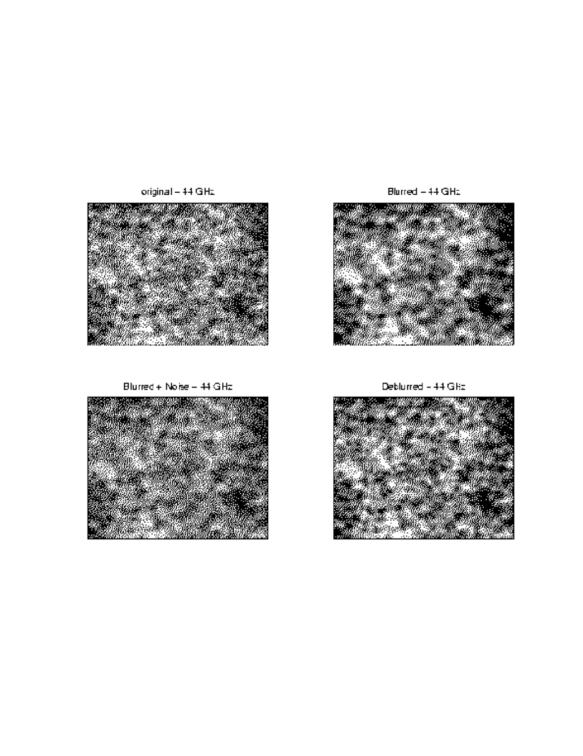
Figure 2: Same as Fig. 1 but at $44\leavevmode\nobreak\ {\rm GHz}$ (see text).

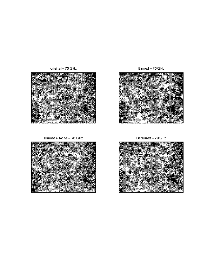
Figure 3: Same as Fig. 1 but at $70\leavevmode\nobreak\ {\rm GHz}$ (see text).

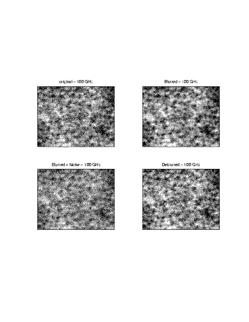
Figure 4: Same as Fig. 1 but at $100\leavevmode\nobreak\ {\rm GHz}$ (see text).

6 A CMB application

We now present tests of the deblurring technique on simulated observations of the PLANCK-LFI. The region analysed is almost identical to the one in Baccigalupi et al. (2000): it is a squared patch ($340\times 340$ pixels) with side of about $20^{\circ}$, centered at $l=90^{\circ}$, $b=45^{\circ}$ (Galactic coordinates). The latitude is high enough that CMB emission dominates over foregrounds, assumed to be represented by synchrotron (Haslam et al. 1982) and dust (Schlegel et al. 1998) emission. We neglect contributions of point sources. The CMB model, in agreement with current experimental results (de Bernardis et al. 2002; Halverson et al. 2002; Lee et al. 2001), corresponds to a flat Friedmann-Robertson-Walker (FRW) metric with a cosmological constant ($70\%$ of the critical density), Hubble parameter today $H_{0}=100h$ km/sec/Mpc with $h=0.7$ baryons at $5\%$ and Cold Dark Matter (25% CDM), with a scale-invariant Gaussian initial spectrum of adiabatic density perturbations.

The PLANCK-LFI instrument works at frequencies $30$, $44$, $70$, and $100\leavevmode\nobreak\ {\rm GHz}$. We assume nominal noise and angular resolution . The maps are blurred through Gaussian PSF’s with circular symmetry and appropriate FWHM’s (i.e., $\approx 33^{\prime}$ at $30\leavevmode\nobreak\ {\rm GHz}$, $\approx 23^{\prime}$ at $44\leavevmode\nobreak\ {\rm GHz}$, $\approx 14^{\prime}$ at $70\leavevmode\nobreak\ {\rm GHz}$, $\approx 10^{\prime}$ at $100\leavevmode\nobreak\ {\rm GHz}$) and summed up together with simulated white noise with rms level as expected for the considered channels. Since we choose to work with a pixel size of about $3.5$ arcminutes, the noise rms are $.042$, $.049$, $.042$ and $.043$ mK in antenna temperature at $30$, $44$, $70$, $100\leavevmode\nobreak\ {\rm GHz}$, respectively.

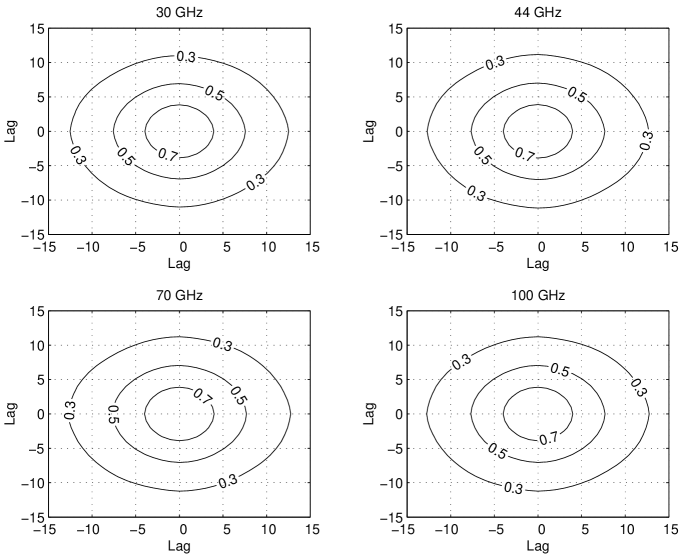
Figure 5: Contour plot of the two-dimensional auto-correlation function of the original simulated CMB maps. Lag in pixels.

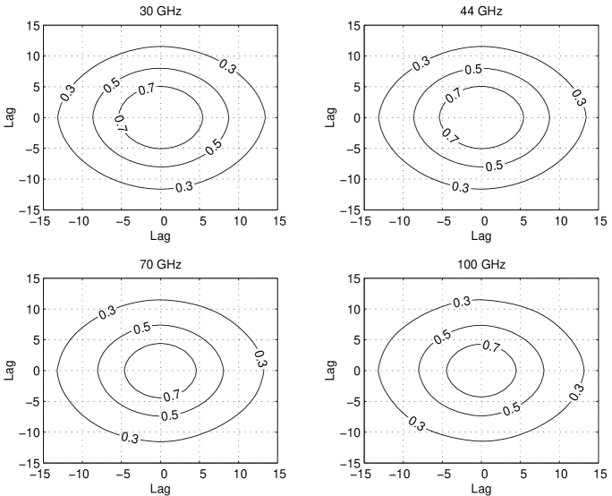
Figure 6: Contour plot of the two-dimensional cross-correlation function of the original with the deblurred CMB maps. Lag in pixels.

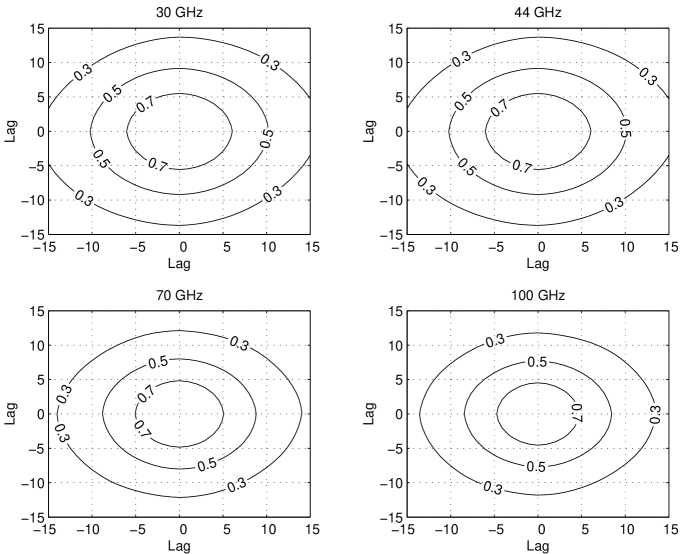
Figure 7: Contour plot of the two-dimensional cross-correlation function of the original with the blurred noise-free CMB maps. Lag in pixels.

Figure 8: One-dimensional cross-section of the two-dimensional Power-spectra in two different frequency ranges of the original $30\leavevmode\nobreak\ {\rm GHz}$ and the deblurred CMB maps (see text). Frequency is in Nyquist units.

The original maps are shown in Figs. 1-4 together with the blurred, blurred plus noise, and deblurred versions (Tikhonov method with reflexive boundary conditions and discrete Laplacian for $\boldsymbol{L}$). The deblurred maps look reasonably good despite the high noise level. But, as expected, there is a clear loss of high frequencies, especially for the lowest frequency maps. This loss, which is intrinsic to any deblurring operation, is important given the high noise level. For example, Figs. 5-7 show, respectively, the two-dimensional auto-correlation function of the original maps and their two-dimensional cross-correlation functions with the blurred (but noise-free) and the deblurred maps. These figures show that the deblurring operation provides good results for the lowest contour levels (those mainly determined by the lowest frequencies) and worse results for the highest contour levels ( those determined mainly by the highest frequencies). The same effect can also be seen in Fig. 8, which shows a one-dimensional cross-section of the power-spectrum of the original $30\leavevmode\nobreak\ {\rm GHz}$ and of the deblurred maps.

The performance of the deblurring procedure can be also checked through the angular power spectrum, which, as usual, is defined by the expansion coefficients $C_{\ell}$ of the two point correlation function in Legendre polynomials. Here $\ell$ is the multipole associated to an angular scale of about $180/\ell$ degrees. Consequently, our analysis applies to $\ell$ ranging from $\ell\simeq 200$, corresponding to the degree scale (larger angles are poorly probed due to the finite extension of our patches), up to multipoles corresponding to the instrumental resolution at each frequency.

Estimates of the $C_{\ell}$ coefficients for the original, blurred, blurred noisy, and deblurred maps are shown in Figs. 9-12. Four CMB acoustic peaks are clearly seen in the original spectrum at $\ell\simeq 200,500,800,1100$. Since we are analysing a limited part of the sky, sample variance causes oscillations in the coefficients, with increasing amplitude as the angular scale approaches the size of the patch, corresponding to the low multipole tail.

Figure 9: Angular power spectrum in different steps of the analysis at 30 GHz. In the top left panel the plot also shows the shape of the instrumental PSF in harmonic space (dotted line).

Figure 10: Same as Fig. 9 but at 44 GHz.

Figure 11: Same as Fig. 9 but at 70 GHz.

Figure 12: Same as Fig. 9 but at 100 GHz.

As shown in the top panels of Figs. 9-12, the $C_{\ell}$ are increasingly affected as the frequency decreases; the increasing tail at high multipoles is the effect of the instrument noise. In all four cases the deblurring procedure has two main effects. First, it restores amplitude and shape of the part of the spectrum not dominated by effects of instrument noise and PSF. Second, as expected from Figs. 5-7, it reconstructs part of the power where the PSF causes a major degradation. In the 30 GHz case, the reconstruction is better in the multipole range $300\leq\ell\leq 400$. Similarly, at $44\leavevmode\nobreak\ {\rm GHz}$, anisotropy power is reconstructed up to $\ell\simeq 500$, and up to $\ell\simeq 700$ at $70$ GHz. Finally, at $100$ GHz part of the original power is recovered up to $\ell\simeq 800$.

Repeting the same simulations with PSFs of elliptical symmetry gives similar results.

In Summary, in all four channels the deblurring procedure was effective in recovering spectral properties of the maps. Although these results have been obtained under the restrictive assumptions of white noise, the characteristics of the deblurring procedure shown above are encouraging and deserve more attention and development in future work.

A last comment regarding component separation. In principle, the separation can be obtained if maps of the same regions are available at different frequencies (Maino et al. 2002; Hobson et al. 1998). In practice, this problem is technically difficult and is far from being solved. Its treatment is beyond the scope of this paper, but the important point is that maps must have the same spatial resolution in order to carry out the separation. This does not imply, however, that maps have to be deblurred to a common resolution. One can also achieve a common resolution by blurring (smoothing). That is, we take Eq. (7) and apply a frequency dependent smoothing operator $\boldsymbol{S}$ to both sides

$${\boldsymbol{\tilde{g}}}=\boldsymbol{S}\boldsymbol{g}=\boldsymbol{S}\boldsymbol{f}+\boldsymbol{S}\boldsymbol{z}={\boldsymbol{\tilde{f}}}+{\boldsymbol{\tilde{z}}}.$$ (23)

Component separation can be done using the different estimates of $\boldsymbol{\tilde{f}}$ obtained by smoothing the maps of different frequencies. But without prior information on $\boldsymbol{\tilde{f}}$ the best linear estimates are simply the maps $\boldsymbol{\tilde{g}}$. To include some prior information we can use smoothness constraints via Tikhonov regularization. The problem thus reduces to the case we have considered before with the difference that this time the noise $\boldsymbol{\tilde{z}}$ is correlated due to the effect of $\boldsymbol{S}$. Depending on the noise structure, one may be able to model correlated noise in Tikhonov regularization using what is known as mixed effects models, some examples can be found in Ma & Gu (2002) and Robinson (1991). If the noise is stationary, one can deconvolve in the frequency domain but again, when the signal spectrum is unknown we may want to regularize the problem using Tikhonov in the frequency domain.

7 An example of deblurring effects on non-Gaussianity

An important point in CMB research is the detection of non-Gaussianity. It is therefore of interest to check the effects of the deblurring procedure on the non-Gaussian characteristics of a map.

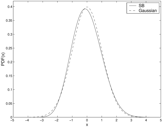
Figure 13: Probability density function used in the simulation of the non-Gaussian random fields (see text). It corresponds to a SB distribution belonging to the Johnson’s parametric family (see Vio et al. 1994).

Experimental results have not yet found any evidence of non-Gaussianity in CMB maps. It is even difficult to conduct realistic simulations of non-Gaussian CMB maps since it is not clear what type of non-Gaussian behavior one should look for. As an example, we consider the effects of deblurring on the marginal distribution of a particular homogeneous non-Gaussian random field whose marginal distribution is slightly different from a Gaussian (skewness $\simeq 0.22$ and kurtosis $\simeq-0.11$ – see Fig. 13). The field has the same autocorrelation function, PSF (with circular symmetry) and $S/N$ of the Gaussian fields simulated in Sect. 5. Realizations of this field are simulated via the method presented in Vio et al. (2001). Skewness and kurtosis coefficients (normalized to be zero for a Gaussian distribution) are calculated for each simulation.

Table 5 presents the average change, from the original values, in skewness and kurtosis over 100 simulations. As expected, noise and blurring have the effect of “Gaussianizing” the random fields (i.e., the estimated skewness and kurtosis are closer to zero than the original values), with obvious consequences on the response of any non-Gaussianity test. Deblurring noticeably improves estimates.

These results, together with the power spectrum reconstruction discussed before, provide a further indication of the usefulness of deblurring in the analysis of CMB maps.

map	$\Delta$ skewness	$\Delta$ kurtosis
30 GHz, blurred	$-0.052\pm 0.058$	$+0.022\pm 0.123$
30 GHz, blurred noisy	$-0.098\pm 0.029$	$+0.055\pm 0.054$
30 GHz, deblurred	$-0.035\pm 0.024$	$+0.032\pm 0.054$
44 GHz, blurred	$-0.038\pm 0.040$	$+0.021\pm 0.087$
44 GHz, blurred noisy	$-0.088\pm 0.017$	$+0.054\pm 0.031$
44 GHz, deblurred	$-0.030\pm 0.019$	$+0.025\pm 0.042$
70 GHz, blurred	$-0.024\pm 0.024$	$+0.016\pm 0.053$
70 GHz, blurred noisy	$-0.078\pm 0.008$	$+0.051\pm 0.018$
70 GHz, deblurred	$-0.024\pm 0.014$	$+0.020\pm 0.032$
100 GHz, blurred	$-0.018\pm 0.017$	$+0.012\pm 0.038$
100 GHz, blurred noisy	$-0.074\pm 0.008$	$+0.049\pm 0.020$
100 GHz, deblurred	$-0.022\pm 0.013$	$+0.018\pm 0.027$

Table 5: Mean and standard deviation of the difference between the skewness and kurtosis coefficients of the blurred, blurred+noise, and deblurred non-Gaussian maps with respect to corresponding values (respectively $\approx 0.22$ and $\approx-0.11$) of the original map (see text). The results are based on 100 simulations with $S/N=2$.

8 An example of deblurring with spatially varying PSF

Although the PSF of PLANCK’s instrument is designed to be spatially invariant, this condition may change after launch, and there may be other experiments that require more general deblurring methods that can be used with spatially varying PSF.

In principle, a real space approach to restoring an image degraded by a spatially variant PSF can be developed, but in practice the methods are quite difficult to implement. Indeed, efficient implementations are currently available for iterative methods (Nagy & O’Leary 1997), but direct algorithms similar to those presented in previous sections for invariant PSFs have not been developed yet. We are presently working on this problem. To illustrate the importance of pursuing this work, we present some simulation results that use an iterative method to restore an image blurred by a spatially variant PSF.

As claimed in Sect. 4.1, one of the most serious difficulties with iterative methods is in the choice of an appropriate stopping criteria. Though methods such as the discrepancy principle, L-curve and GCV can be used, our success with these approaches on CMB maps has been marginal. Without an efficient method for choosing a regularization parameter, or for determining an appropriate stopping criteria, iterative methods may not be the ideal choice for CMB maps. However, because matrix-vector multiplications with $\boldsymbol{H}$ and $\boldsymbol{H}^{T}$ (the most expensive part in the iteration procedure) can be done efficiently for spatially varying PSF (Nagy & O’Leary 1997), iterative methods do give us a means of determining if better restorations can be obtained with a spatially varying model.

To construct a test example, we have used a PSF that changes linearly across the map as shown in Fig. 14. Deblurring was done using a standard conjugate gradient iterative method (Hansen 1997), stopping the iteration when the computed restoration is closest, in a mean square sense, to the true image. The matrix $\boldsymbol{H}$ modelling the spatially varying PSF is constructed by assuming that it is approximately spatially invariant in small regions. If the corresponding, spatially invariant matrix defined by the PSF in the $i$th region is $\boldsymbol{H}_{i}$, then the spatially varying matrix $\boldsymbol{H}$ is defined as

$$\boldsymbol{H}=\sum_{i=1}^{m}\boldsymbol{D}_{i}\boldsymbol{H}_{i}\,,$$

where the matrices $\boldsymbol{D}_{i}$ are nonnegative diagonal and $\sum\boldsymbol{D}_{i}=\boldsymbol{I}$, where $\boldsymbol{I}$ is the identity matrix. Note that using this $\boldsymbol{H}$ is equivalent to interpolation to match the individual PSFs across the different patches. For example, for piecewise constant interpolation the $j$th diagonal entry of $D_{i}$ is 1 if the $j$th pixel is in region $i$, and 0 otherwise. Efficient matrix vector multiplications with $\boldsymbol{H}$ and $\boldsymbol{H}^{T}$ exploit the sparsity of $\boldsymbol{D}_{i}$ and the spatially invariant structure of $\boldsymbol{H}_{i}$. The implementation details are tedious to describe; we only mention here that the basic idea is related to overlap-add and overlap-save convolution methods, and refer the interested reader to (Nagy & O’Leary 1997) for a description of the algorithms, and to (Lee et al. 2002) for a Matlab implementation.

The matrix $\boldsymbol{H}$ in our simulations was constructed through piecewise constant interpolation of 121 PSFs uniformly distributed across the map. The computed spatially varying restoration and the corresponding spatially invariant restoration are shown in Fig. 15. We have used a signal to noise ratio of $S/N=4$ because the iterative procedure is more sensitive to noise than direct methods. Despite these limitations, Fig. 14 shows the advantage of deblurring with a spatially varying PSF.

9 Discussion and conclusions

We have considered Tikhonov regularization for deblurring CMB maps in real space. Although more demanding from the computational point of view, this approach permits the development of algorithms that are more flexible and robust than those based on frequency-space methods. Furthermore, as shown in Fig. 16, the computational cost can be significantly reduced by carefully implementing the algorithms to take advantage of the characteristic structure of the matrices involved.

We have applied the Tikhonov methodology to simulated skies at typical CMB frequencies. We considered test signals with known statistics, as well as realistic simulations of the CMB sky contaminated by noise whose rms is that expected for the low frequency instrument aboard the PLANCK satellite. This case is particularly interesting for application of a deblurring procedure, as the instrument observes the sky at 30, 44, 70 and 100 GHz with very different PSFs of resolution $33$, $22$, $14$, $10$ arcminutes.

We analysed the effects of the deblurring procedure by studying different characteristics of the restored image. Contour plots of the two-dimensional cross-correlation functions of the original and the deblurred maps show that the algorithm effectively improves the resolution, especially that of the worst resolution channels at 30 and 44 GHz. The same effect can be seen in the multipole coefficients of the angular power spectra; the original power on angular scales hidden by the instrument’s PSF is recovered on a significant range of multipoles. We also performed an example of skewness and kurtosis recovery by the deblurring procedure. Instrumental noise and PSFs generally have the effect of pushing skewness and kurtosis toward their Gaussian values; deblurring brings these values closer to their true non-Gaussian ones.

On the basis of these promising results, we plan to develop deblurring algorithms based on the methods we have presented. Since Satellite CMB experiments are able to perform all-sky observations, a robust deblurring procedure which is able to work on the whole sphere is conceivable. We also plan to test map based component separation techniques, requiring multifrequency data of the same resolution, on deblurred maps.

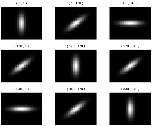
Figure 14: Some of the PSF’s used in the experiment of the variant PSF described in the text. The couple of numbers in the header of each panel provides the coordinates of the pixels to which the displayed PSF corresponds. Each PSF is given by a two-dimensional Gaussian function with ${\rm FWHM}=33\leavevmode\nobreak\ {\rm arcmin}$ along the major axis and ${\rm FWHM}=10\leavevmode\nobreak\ {\rm arcmin}$ along the minor axis. The size of each panel is $23\times 23$ pixels.

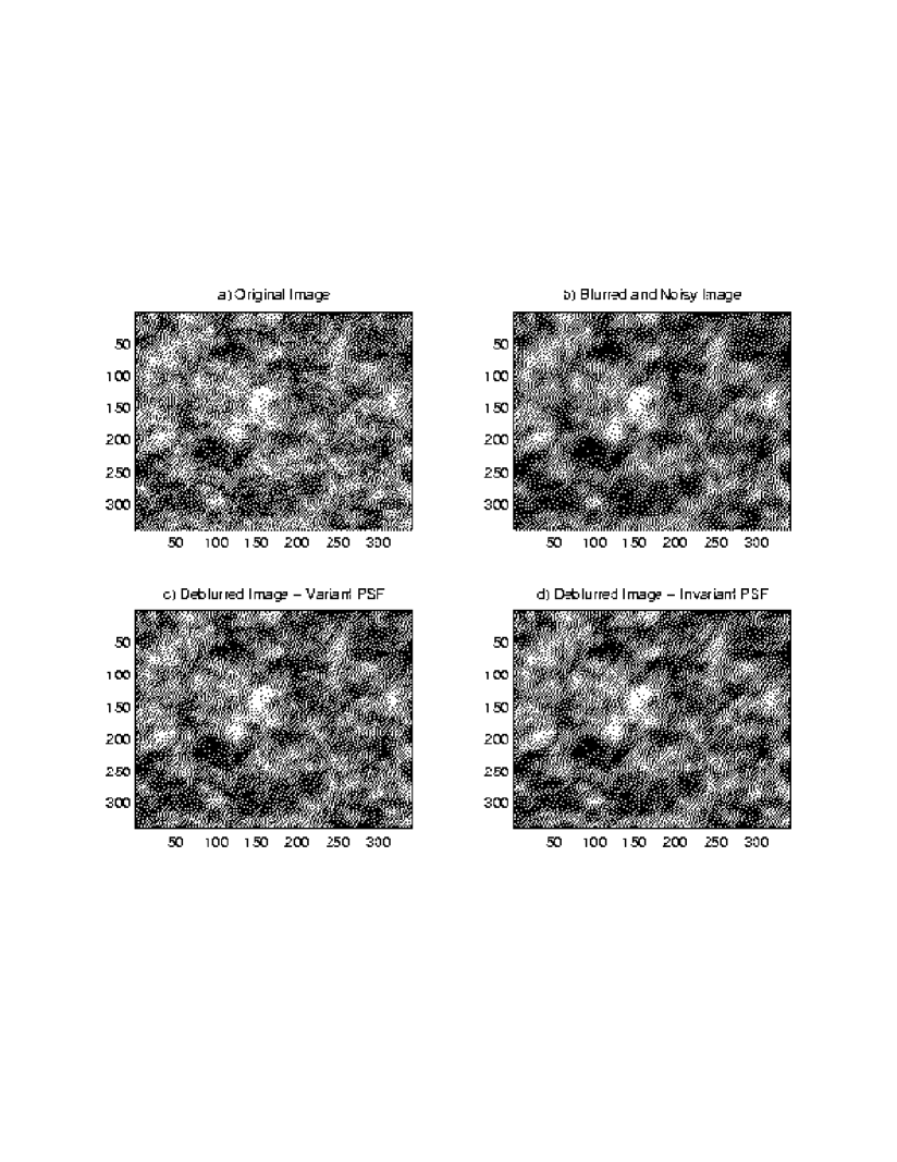
Figure 15: a) original map; b) map obtained by blurring the map in the previous panel with a PSF changing uniformly its orientation across the frame. Some of the PSF’s are shown in Fig. (14). White noise has been added to the map ($S/N=4$); c) map obtained by deblurring with the spatial variant method explained in the text. A set of $121$ PSF’s uniformly distributed across the map have been used; d) map obtained by deblurring with a spatially invariant PSF. The PSF used is that shown in uppermost-left panel in Fig. (14). The standard deviation of the difference between the deblurred and the true maps is $0.41$ for the spatially varying PSF and $0.43$ for the spatially invariant one.

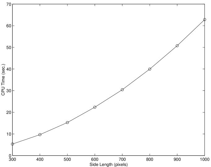
Figure 16: CPU time (sec.) required by the full Tikhonov deblurring procedure of $N\times N$ maps as a function of $N$. The PSF is the one used for the simulations of CMB maps at $30\leavevmode\nobreak\ {\rm GHz}$ (circularly symmetric Gaussian FWHM $\approx 9.5$ pixels). Similar results are obtained for elliptic PSF with ${\rm FWHM}=9.5$ and ${\rm FWHM}=2.8$ pixels along the major and minor axes, respectively, and whose orientations are parallel to the sides of the map. Experiments have been conducted with Matlab 6 on a Pentium IV - $1500\leavevmode\nobreak\ {\rm GHz}$ processor in a Windows 2000 operating system.

Appendix A Automatic choice of the regularization parameter

We briefly describe some methods to estimate the smoothing parameter $\lambda$, which is an essential ingredient in Tikhonov regularization. For further discussions of this topic see Hansen (1997); Tenorio (2001); Vogel (2002).

Since the data $\boldsymbol{g}$ are noisy observations of $\boldsymbol{H}\boldsymbol{f}$, it seems reasonable to choose a value of $\lambda$ that minimizes the predictive mean square error (${\rm PMSE}$),

$${\rm PMSE}(\lambda)=\frac{1}{n}\,\|\,\boldsymbol{H}\boldsymbol{f}-\boldsymbol{H}\boldsymbol{f}_{\lambda}\,\|^{2}.$$ (24)

But since $\boldsymbol{f}$ is unknown, we minimize instead a cross-validation (CV) estimate of (24) obtained by plugging in (24) the data as a proxy for $\boldsymbol{H}\boldsymbol{f}$ and a leave-one-out estimate for $\boldsymbol{H}\boldsymbol{f}_{\lambda}$. The result can be written as

$${\rm CV}(\,\lambda\,)=\frac{1}{n}\,\sum_{i=1}^{n}\left(\frac{g_{i}-\widehat{g}_{i,\lambda}}{1-\boldsymbol{{\cal H}}_{ii}(\lambda)}\right)^{2},$$ (25)

where $\boldsymbol{{\cal H}}_{ii}(\lambda)$ are the diagonal elements of the “hat” matrix (22) that maps $\boldsymbol{g}$ into $\boldsymbol{\widehat{g}}_{\lambda}=\boldsymbol{{\cal H}}\boldsymbol{f}_{\lambda}$. The CV estimate of $\lambda$ is the value that minimizes ${\rm CV}(\lambda)$.

The generalized cross-validation (GCV) function is a “smoothed” version of ${\rm CV}$ in which the diagonal elements of $\boldsymbol{{\cal H}}(\lambda)$ are replaced by their average

$${\rm GCV}(\lambda)=\frac{\|\,\,\boldsymbol{g}-{\boldsymbol{\widehat{g}}}_{\lambda}\,\,\|_{2}^{2}/n}{(\,1-\,{\rm trace}\,\boldsymbol{{\cal H}}(\lambda)/n)^{2}}.$$ (26)

Unlike cross-validation, ${\rm GCV}$ is invariant under orthogonal transformations of the data.

A slight modification of GCV provides and estimate $\widehat{\sigma}^{2}$ of the noise variance $\sigma^{2}$

$$\widehat{\sigma}^{2}=\frac{\|\,\,\boldsymbol{g}-{\boldsymbol{\widehat{g}}}_{\lambda}\,\,\|_{2}^{2}}{n-\,{\rm trace}\,\boldsymbol{{\cal H}}(\lambda)}.$$ (27)

This is just a normalized residual sum of squares where the effective degrees of freedom is determined by the trace of $\boldsymbol{{\cal H}}(\lambda)$.

The L-curve method (Hansen 1997) is another way to determine a balance between goodness of fit and roughness. As $\lambda>0$ increases, the points

$$C(\lambda)=(\,\,\|\,\boldsymbol{g}-\boldsymbol{H}\boldsymbol{f}_{\lambda}\,\|,\,\,\|\boldsymbol{L}\,\boldsymbol{f}_{\lambda}\,\|\,\,)$$ (28)

define a convex curve on the plane that in the log-scale resembles the letter “L”. The selection of $\lambda$ corresponds to the “corner” value where $C(\lambda)$ has the highest curvature.

In general, estimates of $\lambda$ based on cross-validation are robust to small deviations from the homogeneous variance and Gaussian assumptions and, for large samples, converge to the optimal minimizer of the PMSE (Wahba 1990). When the ${\rm GCV}$ function is almost flat around its minimum, it may lead to very small values of $\lambda$ (undersmoothing). A lower limit on $\lambda$ that controls undersmoothing can be achieved by multiplying the trace term in (26) by a constant $k>1$ (Friedman & Silverman 1989; Gu 2002).

The L-curve has not been studied as much as GCV but some studies seem to indicate that L-curve estimates have the same good properties of GCV and, in addition, may be more robust to correlated noise (Hansen 1997). Note, however, that Vogel (1996) has pointed out some convergence problems with L-curve estimates.

Appendix B Efficient implementation of the Tikhonov algorithms

B.1 Exploiting the structure of $\boldsymbol{H}$ and $\boldsymbol{L}$

The efficiency of our approach to computing a minimum of the ${\rm GCV}$ function (21), and to solving the least squares problem (20), is based on exploiting structure of the matrices $\boldsymbol{H}$ and $\boldsymbol{L}$. We assume that $\boldsymbol{L}$ is a structured matrix, such as given in Eq. (15).

Fast algorithms for certain structured matrices arising in image deblurring are well known. For example, when using periodic boundary conditions with a spatially invariant blur, the matrices $\boldsymbol{H}$ and $\boldsymbol{L}$ are BCCB, and therefore have the spectral factorizations

$$\boldsymbol{H}=\boldsymbol{{\cal F}}^{*}\boldsymbol{\Sigma}\boldsymbol{{\cal F}}\,,\quad\boldsymbol{L}=\boldsymbol{{\cal F}}^{*}\boldsymbol{\Delta}\boldsymbol{{\cal F}}\,.$$ (29)

Here, $\boldsymbol{{\cal F}}=\boldsymbol{F}_{N}\otimes\boldsymbol{F}_{M}$ with “$\otimes$” the Kronecker product and $\boldsymbol{F}_{L}$ the one-dimensional Fourier matrix that is a complex, unitary, and symmetric matrix whose elements are given by

$$(F_{L})_{ij}={\rm e}^{-2\pi\iota(i-1)(j-1)/L},$$ (30)

$N$ and $M$ are, respectively, the number of rows and columns of the image, $\boldsymbol{{\cal F}}^{*}$ is the complex conjugate transpose of $\boldsymbol{{\cal F}}$, and $\boldsymbol{\Sigma}$ and $\boldsymbol{\Delta}$ are diagonal matrices containing the eigenvalues of $\boldsymbol{H}$ and $\boldsymbol{L}$, respectively. Note that if $\boldsymbol{L}=\boldsymbol{I}$, then $\boldsymbol{\Delta}=\boldsymbol{I}$. The eigenvalues can be obtained by computing a two-dimensional fast Fourier transform (FFT) of the first columns of $\boldsymbol{H}$ and $\boldsymbol{L}$, at a cost of $O(N^{2}\log N)$, assuming the blurred image contains $N\times N$ pixels. Recently, however, many other efficient methods have been proposed that are suited to deal with a large variety of situations.

B.2 Symmetric PSF

If the spatially invariant PSF $h(x,y)$ is symmetric, but not necessarily separable, i.e., $h(x,y)=h(-x,y)=h(x,-y)=h(-x,-y)$, it happens that also the matrix $\boldsymbol{H}$ is symmetric. In this situation, it is possible to show (Ng et al. 1999) that, under reflexive boundary conditions, the matrices $\boldsymbol{H}$ and $\boldsymbol{L}$ have the spectral factorizations

$$\boldsymbol{H}=\boldsymbol{{\cal C}}^{T}\boldsymbol{\Sigma}\boldsymbol{{\cal C}}\,,\quad\boldsymbol{L}=\boldsymbol{{\cal C}}^{T}\boldsymbol{\Delta}\boldsymbol{{\cal C}}\,,$$ (31)

where $\boldsymbol{{\cal C}}$ is the orthogonal two-dimensional discrete cosine transform (DCT) matrix, and $\boldsymbol{\Sigma}$ and $\boldsymbol{\Delta}$ are diagonal matrices containing the eigenvalues of $\boldsymbol{H}$ and $\boldsymbol{L}$, respectively. In this case, the eigenvalues of $\boldsymbol{H}$ are given by

$$\sigma_{i}=\frac{\left[\boldsymbol{{\cal C}}\boldsymbol{H}\boldsymbol{e}_{1}\right]_{i}}{\left[\boldsymbol{{\cal C}}\boldsymbol{e}_{1}\right]_{i}}\,,$$ (32)

where $\boldsymbol{e}_{1}^{T}=\left[\begin{array}[]{cccc}1&0&\cdots&0\end{array}\right]$. Note that $\boldsymbol{H}\boldsymbol{e}_{1}$ is the first column of $\boldsymbol{H}$, which can be constructed from the PSF, and that multiplication by $\boldsymbol{{\cal C}}$ can be done in $O(N^{2}\log N)$ operations using fast DCT algorithms. Computing the eigenvalues $\delta_{i}$ of $\boldsymbol{L}$ is done in a similar manner.

To efficiently compute the regularization parameter, we first replace $\boldsymbol{H}$ and $\boldsymbol{L}$ with their spectral factorizations in Eq. (21), and simplify to obtain

$${\rm GCV}(\lambda)=n\sum_{i=1}^{n}\left(\frac{\hat{g}_{i}\delta_{i}^{2}}{\sigma_{i}^{2}+\lambda^{2}\delta_{i}^{2}}\right)^{2}/\left(\sum_{i=1}^{n}\frac{\delta_{i}^{2}}{\sigma_{i}^{2}+\lambda^{2}\delta_{i}^{2}}\right)^{2}$$ (33)

where, in the case of reflexive boundary conditions, ${\boldsymbol{\widehat{g}}}=\boldsymbol{{\cal C}}\boldsymbol{g}$, and $n=N^{2}$ is the number of pixels in the image. We can now use standard minimization algorithms, such as Newton’s method, to find the value of $\lambda$ that minimizes the scalar value function (33). In the computations reported in this paper, we used Matlab’s fminbnd function, which is based on Golden Section search and parabolic interpolation.

We can also use the spectral factorization to efficiently solve the least squares problem (20). Because ${\cal C}$ is an orthogonal matrix, (20) is equivalent to

$$\min\left\|\left(\begin{array}[]{c}\boldsymbol{\Sigma}\\ \lambda\boldsymbol{\Delta}\end{array}\right)\boldsymbol{\widehat{f}}-\left(\begin{array}[]{c}\boldsymbol{\widehat{g}}\\ \boldsymbol{0}\end{array}\right)\right\|_{2}\,,$$ (34)

where $\boldsymbol{\widehat{f}}=\boldsymbol{{\cal C}}\boldsymbol{f}$ and $\boldsymbol{\widehat{g}}=\boldsymbol{{\cal C}}\boldsymbol{g}$ (that is, $\boldsymbol{\widehat{f}}$ and $\boldsymbol{\widehat{g}}$ are, respectively, DCTs of $\boldsymbol{f}$ and $\boldsymbol{g}$). Because $\boldsymbol{\Sigma}$ and $\boldsymbol{\Delta}$ are diagonal matrices, this least squares problem can be solved, using a sequence of Givens rotations, with only $O(N^{2})$ operations (Hansen 1997). In fact, strategic Givens rotations permits to change the structure of matrix

$$\left(\begin{array}[]{c}\boldsymbol{\Sigma}\\ \lambda\boldsymbol{\Delta}\end{array}\right)\longrightarrow\left(\begin{array}[]{cccc}*&&&\\ &*&&\\ &&\ddots&\\ &&&*\\ &&&\\ &*&&\\ &&\ddots&\\ &&&*\end{array}\right)$$ (35)

(“$*$” indicates a non-zero element) to

$$\left(\begin{array}[]{cccc}*&&&\\ &*&&\\ &&\ddots&\\ &&&*\\ &&&\\ &&&\\ &&&\\ &&&\end{array}\right)$$ (36)

which is a form more amenable for an efficient solution.

To summarize, after $\lambda$ is computed by finding the minimum of the ${\rm GCV}$ function, the Tikhonov solution (12) can be computed as follows:

• Construct the first column of $\boldsymbol{H}$ from the PSF

• Use a fast DCT algorithm to compute $\boldsymbol{\Sigma}$.

• Use a fast DCT algorithm to compute $\boldsymbol{\Delta}$.

• Solve the least squares problem (34) to compute $\boldsymbol{\widehat{f}}$.

• Use a fast inverse DCT algorithm to compute $\boldsymbol{f}$ from $\boldsymbol{\widehat{f}}$.

The total cost of this approach is $O(N^{2}\log N)$, and storage requirements are only $O(N^{2})$ (i.e., the storage required for an $N\times N$ image). Specific implementations used for the experiments are available in the Matlab package RestoreTools (Lee et al. 2002) .

We remark that the efficient implementation described above assumes a symmetric $\boldsymbol{H}$ and reflexive boundary conditions. Of course a similar approach can be implemented for periodic boundary conditions, using FFTs in place of DCTs. However, if we want to use reflexive boundary conditions, and $\boldsymbol{H}$ is not symmetric, then other methods should be considered.

B.3 Separable PSF

If the PSF is separable, then $\boldsymbol{H}$ can be decomposed into a Kronecker product,

$$\boldsymbol{H}=\boldsymbol{A}\otimes\boldsymbol{B}=\left(\begin{array}[]{cccc}a_{11}\boldsymbol{B}&a_{12}\boldsymbol{B}&\cdots&a_{1n}\boldsymbol{B}\\ a_{21}\boldsymbol{B}&a_{22}\boldsymbol{B}&\cdots&a_{2n}\boldsymbol{B}\\ \vdots&\vdots&&\vdots\\ a_{m1}\boldsymbol{B}&a_{m2}\boldsymbol{B}&\cdots&a_{mn}\boldsymbol{B}\end{array}\right)\,.$$ (37)

The special block structure of Kronecker products can be exploited is several ways (Jain 1989; Kamm & Nagy 1998a). In particular, assuming the images are $N\times N$ arrays of pixel values, then the following properties hold:

1. The first important property is that we need only store the $N\times N$ matrices $\boldsymbol{A}$ and $\boldsymbol{B}$, and do not need to construct the $N^{2}\times N^{2}$ matrix $\boldsymbol{H}$ explicitly.

2. The $N^{2}\times N^{2}$ linear system

   $$(\boldsymbol{A}\otimes\boldsymbol{B})\boldsymbol{f}=\boldsymbol{g}$$ (38)

   is equivalent to the $N\times N$ matrix equation

   $$\boldsymbol{A}\boldsymbol{F}\boldsymbol{B}^{T}=\boldsymbol{G}\,,$$ (39)

   where the $N^{2}\times 1$ vectors $\boldsymbol{f}$ and $\boldsymbol{g}$ are obtained through a lexicographical ordering of the $N\times N$ arrays $\boldsymbol{F}$ and $\boldsymbol{G}$.

3. The singular value decomposition (SVD) is a tool used for analyzing and solving ill-posed problems (Hansen 1997). It is usually too expensive for large scale problems, such as image deblurring. However, for Kronecker product structures, the SVD can be used efficiently. To see this, suppose

   $$\boldsymbol{A}=\boldsymbol{U}_{a}\boldsymbol{\Sigma}_{a}\boldsymbol{V}_{a}^{T}\quad\mbox{and}\quad\boldsymbol{B}=\boldsymbol{U}_{b}\boldsymbol{\Sigma}_{b}\boldsymbol{V}_{b}^{T}$$ (40)

   are the SVDs of $\boldsymbol{A}$ and $\boldsymbol{B}$. Then

   $$\boldsymbol{A}\otimes\boldsymbol{B}=(\boldsymbol{U}_{a}\otimes\boldsymbol{U}_{b})(\boldsymbol{\Sigma}_{a}\otimes\boldsymbol{\Sigma}_{b})(\boldsymbol{V}_{a}^{T}\otimes\boldsymbol{V}_{b}^{T})$$ (41)

   is the SVD of $\boldsymbol{H}=\boldsymbol{A}\otimes\boldsymbol{B}$. In particular, the SVD of a Kronecker product can be computed at a cost of only $O(N^{3})$, rather than $O(N^{6})$ if working directly with $\boldsymbol{H}$.

Using these properties, it looks like the SVD can be used in place of the the spectral factorization of $\boldsymbol{H}$. However, we run into difficulty if the regularization operator, $\boldsymbol{L}$, is not the identity matrix. To see this, assume that the SVD of $\boldsymbol{H}$ is given by

$$\boldsymbol{H}=\boldsymbol{U}_{H}\boldsymbol{\Sigma}\boldsymbol{V}_{H}^{T}\,,$$ (42)

where $\boldsymbol{U}_{H}=\boldsymbol{U}_{a}\otimes\boldsymbol{U}_{b}$, $\boldsymbol{\Sigma}=\boldsymbol{\Sigma}_{a}\otimes\boldsymbol{\Sigma}_{b}$, and $\boldsymbol{V}_{H}=\boldsymbol{V}_{a}\otimes\boldsymbol{V}_{b}$. In addition, assume $\boldsymbol{L}$ has the SVD

$$\boldsymbol{L}=\boldsymbol{U}_{L}\boldsymbol{\Delta}\boldsymbol{V}_{L}^{T}\,,$$ (43)

where the matrices $\boldsymbol{U}_{H}$, $\boldsymbol{V}_{H}$, $\boldsymbol{U}_{L}$, and $\boldsymbol{V}_{L}$ are orthogonal, and $\boldsymbol{\Sigma}$ and $\boldsymbol{\Delta}$ are diagonal. If $\boldsymbol{L}=\boldsymbol{I}$, then $\boldsymbol{\Delta}=\boldsymbol{I}$, and we can take $\boldsymbol{U}_{L}=\boldsymbol{V}_{L}=\boldsymbol{V}_{H}$. Now Eqs. (33) and (34) can be used with $\boldsymbol{\widehat{f}}=\boldsymbol{V}_{H}^{T}\boldsymbol{f}$ and $\boldsymbol{\widehat{g}}=\boldsymbol{U}_{H}^{T}\boldsymbol{g}$. In this case, by the above properties of Kronecker products, we see that the cost of transforming (21) into (33) and (20) into (34) is $O(N^{3})$. This is slightly more expensive than the $O(N^{2}\log N$) cost when using fast transforms, but it is still a reasonably efficient approach. The storage requirements remain $O(N^{2})$.

A problem arises, though, when trying to use a differentiation operator for $\boldsymbol{L}$ because, in general, $\boldsymbol{V}_{H}\neq\boldsymbol{V}_{L}$. If these two orthogonal matrices are not equal, then (20) cannot be efficiently transformed into (34). Moreover, (21) cannot be efficiently transformed into (33), and so evaluation of the ${\rm GCV}$ function, and hence computation of its minimum, becomes much more expensive. In this difficult situation, a hybrid iterative/direct method (Kilmer & O’Leary 1999) may be appropriate.

Finally, we remark that in general there is no computational difference between separable spatially variant PSFs and separable spatially invariant blurs. That is, efficient direct methods can be used if $\boldsymbol{L}=\boldsymbol{I}$, but not when using a differentiation operator for $\boldsymbol{L}$ (Kamm & Nagy 1998b). Moreover, in the difficult cases when the direct factorization approach cannot be used, iterative and hybrid methods can be implemented very efficiently for both spatially invariant and spatially varying blurs (Hanke & Nagy 1996; Nagy & O’Leary 1997, 1998).

B.4 Non-separable PSF

In this section we have so far described efficient implementations of direct methods for the following situations:

1. Spatially invariant PSF, with periodic boundary conditions. In this case FFTs are used.

2. Spatially invariant and symmetric PSF, with reflexive boundary conditions. In this case fast cosine transforms are used.

3. Separable PSF, invariant or variant. In this case efficient use of the Kronecker product structure is exploited.

If the image deblurring problem does not fit into one of these categories, then some other approach should be used. One possible option is to simplify, or approximate, the problem with one that does fit into one of the above categories. For example, a symmetric approximation, such as $(\boldsymbol{H}+\boldsymbol{H}^{T})/2$, can be used with reflexive boundary conditions so that the fast cosine transform approach can be used. Other, recently developed approaches, use more sophisticated approximation techniques.

In particular the Kronecker approximation method (Kamm & Nagy 1998a, b) is a technique that deserves some attention. The main idea of this method is to approximate the non-separable matrix $\boldsymbol{H}$ with a separable matrix. To see how this can be done, suppose $\boldsymbol{P}$ is an $n\times n$ image of the PSF, with $p_{ij}$ denoting the center (origin) or the PSF. If the PSF is separable, then we can write

$$\boldsymbol{P}={\bf a}{\bf b}^{T}\quad\mbox{and}\quad\boldsymbol{H}=\boldsymbol{A}\otimes\boldsymbol{B}\,,$$ (44)

where:

• Zero boundary conditions imply $\boldsymbol{A}$ and $\boldsymbol{B}$ are Toeplitz matrices defined by ${\bf a}$ and ${\bf b}$, respectively. That is,

  $$\boldsymbol{A}=\left(\begin{array}[]{ccccc}a_{i}&\cdots&a_{1}&&\\ \vdots&\ddots&&\ddots&\\ a_{n}&&\ddots&&a_{1}\\ &\ddots&&\ddots&\vdots\\ &&a_{n}&\cdots&a_{i}\end{array}\right)\,$$ (45)

  and

  $$\boldsymbol{B}=\left(\begin{array}[]{ccccc}b_{j}&\cdots&b_{1}&&\\ \vdots&\ddots&&\ddots&\\ b_{n}&&\ddots&&b_{1}\\ &\ddots&&\ddots&\vdots\\ &&b_{n}&\cdots&b_{j}\end{array}\right)\,.$$ (46)

• Reflexive boundary conditions imply $\boldsymbol{A}$ and $\boldsymbol{B}$ are Toeplitz-plus-Hankel matrices defined by ${\bf a}$ and ${\bf b}$, respectively. That is,

  $$\boldsymbol{A}=\left(\begin{array}[]{ccccc}a_{i}&\cdots&a_{1}&&\\ \vdots&\ddots&&\ddots&\\ a_{n}&&\ddots&&a_{1}\\ &\ddots&&\ddots&\vdots\\ &&a_{n}&\cdots&a_{i}\end{array}\right)+\left(\begin{array}[]{ccccc}a_{i+1}&\cdots&a_{n}&\\ \vdots&\tiny\begin{array}[]{ccc}&&\cdot\\ &\cdot&\\ \cdot&&\end{array}&&\\ a_{n}&&&a_{1}\\ &&\tiny\begin{array}[]{ccc}&&\cdot\\ &\cdot&\\ \cdot&&\end{array}&\vdots\\ &a_{1}&\cdots&a_{i-1}\end{array}\right)\,,$$ (47)

  and

  $$\boldsymbol{B}=\left(\begin{array}[]{ccccc}b_{j}&\cdots&b_{1}&&\\ \vdots&\ddots&&\ddots&\\ b_{n}&&\ddots&&b_{1}\\ &\ddots&&\ddots&\vdots\\ &&b_{n}&\cdots&b_{j}\end{array}\right)+\left(\begin{array}[]{ccccc}b_{j+1}&\cdots&b_{n}&\\ \vdots&\tiny\begin{array}[]{ccc}&&\cdot\\ &\cdot&\\ \cdot&&\end{array}&&\\ b_{n}&&&b_{1}\\ &&\tiny\begin{array}[]{ccc}&&\cdot\\ &\cdot&\\ \cdot&&\end{array}&\vdots\\ &b_{1}&\cdots&b_{j-1}\end{array}\right)\,.$$ (48)

If the PSF is not separable, then we could compute a rank-one approximation of $\boldsymbol{P}$, and construct $\boldsymbol{A}$ and $\boldsymbol{B}$ as described above. That is,

$$\boldsymbol{P}\approx{\bf a}{\bf b}^{T}\quad\Rightarrow\quad\boldsymbol{H}\approx\boldsymbol{A}\otimes\boldsymbol{B}\,.$$ (49)

With a proper weighting applied to $P$, one obtains an optimal approximation of the form

$$\min||\boldsymbol{H}-\boldsymbol{A}\otimes\boldsymbol{B}||_{F}\,,$$ (50)

where $||\cdot||_{F}$ is the Frobenius norm and the minimization is done over all Kronecker products $\boldsymbol{A}\otimes\boldsymbol{B}$. This approximation can be computed in $O(n^{3})$ operations; see Kamm & Nagy (1998a, b) for further details.