Twofold effect of Alfvén waves on the transverse gravitational instability

This paper is devoted to the study of the gravitational instability of a medium permeated by a uniform magnetic field along which a circularly polarized Alfvén wave propagates. We concentrate on the case of perturbations purely transverse to the ambient field by means of direct numerical simulations of the MHD equations and of a linear stability analysis performed on a moderate amplitude asymptotic model. The Alfvén wave provides an extra stabilizing pressure when the scale of perturbations is sufficiently large or small compared with the Jeans length $L_{J}$. However, there is a band of scales around $L_{J}$ for which the Alfvén wave is found to have a destabilizing effect. In particular, when the medium is stable in absence of waves, the gravitational instability can develop when the wave amplitude lies in an appropriate range. This effect appears to be a consequence of the coupling between Alfvén and magnetosonic waves. The prediction based on a WKB approach that the Alfvén wave pressure tensor is isotropic and thus opposes gravity in all directions is only recovered for large amplitude waves for which the coupling between the different MHD modes is negligible.

1 Introduction

Formation of the largest clouds in the interstellar medium (ISM) certainly rely on ram pressure of large-scale turbulent flows (Vázquez-Semadeni et al. (1995)), whereas molecular clouds most likely owe their stability to internal turbulent motions. It is thus of importance for the understanding of the ISM dynamics, to study the gravitational instability in media stirred by MHD turbulence. Since the first stability analysis by Jeans (Jeans (1902)), there has been a series of studies of the onset of gravitational instabilities in rotating, magnetized or turbulent media (e.g. Chandrasekhar (1961); Toomre (1964), Elmegreen (1991)). Neutral turbulence was shown to oppose gravity by a turbulent pressure if its characteristic scale is small enough compared to the instability wavelength (Chandrasekhar (1951)). In comparison with the mechanism that generates density fluctuations, turbulent pressure is however a higher order effect (Sasao (1973)). Later studies predict a reversal of the Jeans’ criterium if the turbulent spectrum is shallow enough (Bonazzola et al. (1987); Vázquez-Semadeni & Gazol (1995)). Numerical simulations in two dimensions confirm that highly compressible turbulence can have both a stabilizing effect for long-wavelength perturbations and a destabilizing one at small scales (Léorat et al. (1990)).

Consideration of MHD turbulence is crucial in the study of star formation. As is well known, magnetic fields are ubiquitous in the ISM and they are believed to be one of the major agents controlling star formation (e.g. Shu et al. (1987)). If the value of the ambient magnetic field (supposed to be relatively smooth over the large scales) is large enough (sub-critical regime), overall collapse is hindered and the interstellar matter gathers under a quasi-static contraction due to ambipolar drift until a super-critical core is formed : this is the low-mass star formation process. On the contrary, if the magnetic field is weak, matter can easily become gravitationally unstable and high-mass stars form in a rapid collapsing process (Mouschovias (1991)). In this picture turbulence is considered as an additional pressure against gravity. This pressure could be provided by turbulent magnetic field fluctuations.

In the previous picture the interactions between the turbulent motions and the magnetic field are however not consistently taken into account and it is legitimate to wonder whether this star formation scenario still holds in a fully turbulent case. The key point in this bi-modal star formation theory is that magnetic fields always oppose gravitational instabilities, at least in the linear regime. A uniform magnetic field is known to increase the critical wavelength for instability by a factor $({\beta/1+\beta})^{-1/2}$ (where $\beta$ is up to a constant, the ratio of thermal over magnetic pressure) if the perturbation is exactly perpendicular to the ambient field, whereas it has no effect in every other direction. Support along the magnetic field is provided by Alfvén waves (AWs). Recent linear stability analyses indeed show that AWs provide an extra pressure for perturbations parallel to the background field and as a result the Jeans length can be arbitrarily increased for sufficiently large wave amplitude (Lou (1996); Fukuda & Hanawa (1999)). Numerical simulations in a slab geometry have confirmed this result for a spectrum of AWs (Gammie & Ostiker (1996)). However, higher dimensional models including decaying MHD turbulence (e.g. Stone et al. (1998); Ostriker et al. (1999)) have shown that in magnetically supercritical clouds the time for gravitational collapse does not depend on the initial level of turbulence. In high resolution three dimensional MHD simulations, the presence of short wavelength MHD waves appears to be able to delay the collapse (Heitsch et al. (2001))

Other studies by Pudritz (1990) and McKee & Zweibel (1995) use a WKB theory Dewar (Dewar 1970) to argue that the AW pressure tensor is isotropic and that these waves provide an additional support in every direction. The phenomenological argument is based on the observation that the pressure tensor of the waves $P_{W}=\frac{\delta B^{2}}{8\pi}{\bf I}-\frac{\delta{\bf B}\delta{\bf B}}{4\pi}+\rho\delta{\bf v}\delta{\bf v}$ reduces to $P_{W}=\frac{\delta B^{2}}{8\pi}{\bf I}$ since for a traveling AW, the equations of motion imply that $\delta{\bf v}=\pm\frac{\delta{\bf B}}{(4\pi\rho)^{1/2}}$. This conclusion is however based on the assumption that the only waves propagating in the medium are pure AWs. Even though AWs are certainly the only kind of MHD waves that can propagate over large distances due to their quasi-non-dissipative properties (they are transverse waves), as soon as they are perturbed, they generate long wavelength magnetosonic waves. The latter are intrinsically coupled to AWs and can drastically change the global response of AWs under an external compression.

In this paper, we address the simple question of the linear stability of a self-gravitating medium permeated by a uniform magnetic field ${\cal B}_{0}$ along which a finite amplitude circularly polarized AW propagates. In particular, we study the case in which perturbations are transverse to the uniform magnetic field. We first present a numerical test showing that for transverse perturbations, the presence of a longitudinal AW does not always provide an additional support against gravitational collapse. In order to explain this result we have done a linear stability analysis. Due to the presence of several kinds of instabilities taking place at different scales (e.g. decay instability (Goldstein (1978); Derby (1978))) and the coupling between them, the three dimensional analysis performed on the complete MHD equations appears to be cumbersome and physically unclear. In fact this problem, which leads to linear equations with periodically varying coefficients, requires a Floquet analysis. When the perturbations are parallel to the AW, the infinite hierarchy of dispersion relations obtained in this way decouples into a set of physically equivalent dispersion relations (Jayanti & Hollweg (1993)). However, when perturbations have an arbitrary direction with respect to the propagation direction of the AW, the modes remain coupled and the hierarchy of dispersion relations needs to be truncated. Even in this case the resulting dispersion relation is very complicated (Viñas & Goldstein (1991) obtain a 78 order polynomial). For this reason we perform a linear stability analysis on a reduced description of the MHD equations based on long wavelength, small amplitude perturbative expansion (Gazol et al. (1999)).

The plan of the paper is as follows. In Section 2 we present the numerical results. The reduced system of equations used for the theoretical interpretation of these results is described in Section 3. Its derivation is presented in the Appendix, and its linear stability analysis in Section 4. Section 5 is a conclusion.

2 Numerical Simulations

In this section we present direct numerical simulations of the self-gravitating 2.5D MHD equations

$$\partial_{t}\rho+{\bf\nabla}\cdot(\rho{\bf u})=0$$ (1)

$$\rho(\partial_{t}{\bf u}+{\bf u}\cdot{\bf\nabla}{\bf u})=-\frac{\beta}{\gamma}{\bf\nabla}\rho^{\gamma}+({\bf\nabla}\times{\bf b})\times{\bf b}$$

$$\;\;\;\;\;\;\;\;\;\;\;\;\;\;\;\;\;\;\;\;\;\;\;\;\;\;-\beta J^{2}\rho\nabla\Phi$$ (2)

$$\partial_{t}{\bf b}-{\bf\nabla}\times({\bf u}\times{\bf b})=0$$ (3)

$${\bf\nabla}\cdot{\bf b}=0$$ (4)

$$\nabla^{2}\Phi=\rho-1,$$ (5)

where all variables have been adimensionalized using as velocity unit, the Alfvén speed $v_{A}={\cal B}_{0}/(4\pi\rho_{0})^{1/2}$, with ${\cal B}_{0}$ and $\rho_{0}$ being the ambient magnetic field, chosen to point along the x-axis, and the average density respectively. In equation (2) $\gamma$ denotes the polytropic gas constant, $\beta=c_{s}^{2}/v_{A}^{2}$ with $c_{s}$ the sound speed, and $J$ denotes the Jeans number, ratio of the characteristic scale $L_{0}$ to the Jeans length $L_{J}=(\pi c_{s}^{2}/G\rho_{0})^{1/2}$. The simulations have been performed using a pseudo-spectral code with a resolution of $128^{2}$ grid points, except when otherwise specified.

Previous numerical work in more than one space dimension have mainly addressed the influence of AWs on the gravitational collapse in a turbulent context. In order to clearly identify the AW pressure contribution we choose here to study the gravitational instability close to threshold in presence of a parallel propagating, right-hand circularly polarized AW which is an exact solution even in the presence of gravity. We focus on the case of purely transverse perturbations and thus choose the longitudinal size of the computational domain $L_{x}$ to be slightly smaller than $L_{J}$ so that the system is stable in the direction along the uniform magnetic field. The critical transverse size of the domain is

$$L_{\perp J}=\frac{2\pi}{J}\left(\frac{1+\beta}{\beta}\right)^{1/2}.$$

In all subsequent simulations we fix $\gamma=5/3$, $J=1$ and just vary the transverse scale $L_{\perp}$. The AW of amplitude $B_{0}$ reads $b_{y}+ib_{z}=(\omega/k)u_{y}+iu_{z}=B_{0}e^{i(kx-\omega t)}$, $\rho=1$ and $u_{x}=0$, where for the nondispersive case $\omega=k$. The wave number is usually taken as $k=1$ and a noise of $10^{-7}$ in the first five Fourier modes is superimposed on the uniform density.

We first consider the case $\beta=0.5$, for which perturbations at scales $L_{\perp}>L_{\perp J}=2\pi\sqrt{3}$ are gravitationally unstable in the absence of waves. Choosing $L_{\perp}/2\pi=1.74$ and $L_{x}/2\pi=0.948$ a series of six simulations varying the wave amplitude has been performed. When $B_{0}=0$ the growth rate of the gravitational instability is verified to agree within 1% with the theoretical value $0.068$. Increasing $B_{0}$ by steps of 0.1, the growth rate is first observed to increase up to $0.107$ for $B_{0}=0.3$. It then decreases until $B_{0}=0.5$ for which the system becomes stable. This result confirms that a large enough amplitude AW successfully stabilizes the medium against the gravitational instability. However it is surprising that the growth rate increases for small wave amplitudes.

Figure 1: $|\ln\rho_{k}(0,1)|$ as a function of time for $\beta=0.5$, $L_{x}/2\pi=0.95$, $L_{\perp}/2\pi=1.7$ and $B_{0}=0.3$

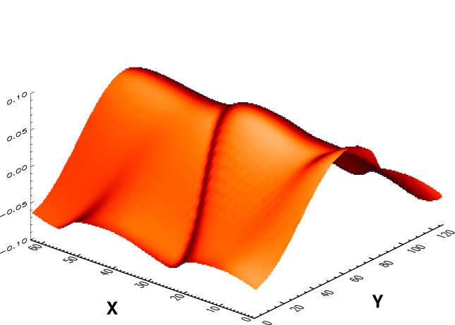
Figure 2: Density field fluctuations for $\beta=0.5$, $L_{x}/2\pi=0.95$, $L_{\perp}/2\pi=1.7$ and $B_{0}=0.3$, at $t=288$

Figure 3: $|\ln\rho_{k}(0,1)|$ as a function of time for $\beta=2.0$, $L_{x}/2\pi=0.7$, $L_{\perp}/2\pi=1.21$ and $B_{0}=0.3$

This suggests to study the behavior of the gravitationally stable system in presence of an AW. Numerical simulations are now performed with a resolution of $64\times 128$ grid points for $L_{x}/2\pi=0.95$ and $L_{\perp}/2\pi=1.7$ so that the medium is gravitationally stable. The system remains stable in presence of the AW as long as the wave amplitude does not exceeds 0.16 but becomes unstable in the range of amplitudes $[0.18,0.35]$. Figure 1 shows the typical temporal behavior of $|\ln\rho_{k}(0,1)|$, where $\rho_{k}(k_{x},k_{y})$ denotes the Fourier coefficient of the density, for an unstable simulation. In Fig. 2 the density field fluctuations $\rho-1$ resulting from the same simulation are displayed at $t=288$. In addition to the concentration of mass in the transverse direction, a weak longitudinal modulation is also visible. Another set of simulations with $\beta=2$, $L_{x}/2\pi=0.7$ and $L_{\perp}/2\pi=1.21$, shows the same behavior with respect to the gravitational instability but in this case, the growth of the gravitational instability, shown in Fig. 3, is oscillatory.

Similar results are also obtained when choosing the AW wave number on the third Fourier mode. However in the case $\beta<1$, larger wave numbers or smaller values of $\beta$ lead to stronger longitudinal modulation resulting from the coexistence with the decay instability.

In the next two sections we present an analytical interpretation of the previous results.

3 Reduced description

As mentioned in Sect. 1 the analytical study of the transverse gravitational stability of the system is a very complex problem. Its solution would require numerical simulations of the same complexity as the ones done in the previous section. For this reason and in order to gain some physical insight, we use a reduced description adapted to study the nonlinear dynamics of an AW propagating along a strong uniform field coupled with a small amplitude MHD flow in planes perpendicular to this field. This reduced description has been derived in the absence of self-gravity by Gazol et al. (1999) (see also Champeaux et al. (1999)) for two different regimes depending on the values of $\beta$ and its derivation is presented in Appendix A for the self-gravitating case. A verification of this asymptotic description has been performed in the context of Hall MHD for the development of transverse instabilities on a moderate amplitude AW (Laveder et al. 2002b ). Here we only consider the case $\beta\neq 1$, for which the reduced equations have been extended to take into account the coupling with magnetosonic waves. The case where $\beta$ is close to the resonance $\beta=1$ is more delicate as both the AW and the sonic wave must be considered on an equal footing and obey nonlinear equations. The derivation is based on the existence of a small parameter $\epsilon$, squared ratio of the wave amplitude to the value of the strong uniform magnetic field, that identifies with the squared Alfvenic Mach number, $M_{A}^{2}=u_{0}^{2}/v_{A}^{2}$, where $u_{0}$ is a typical velocity fluctuation. In the frame of reference of the AW, a stretching of coordinates allows to study non-linear effects on long times, $\tau=\epsilon^{2}t$ and large scales, $(\xi,\eta,\zeta)=(\epsilon(x-t),\epsilon^{3/2}y,\epsilon^{3/2}z)$, for both the AW and the transverse MHD flow. The scaling and the resulting equations are given in Appendix A. The coupling between the AW and the transverse hydrodynamics is accomplished through the introduction of mean transverse velocity and magnetic fields which describe the slow transverse dynamics and result from the average over the direction of the uniform magnetic field.

Within the framework of this description, where the small-scale magnetosonic waves have been filtered, it is possible to study the interplay between the AW and the large-scale transverse gravito-magneto-acoustic mode in isolation from the other small-scale instabilities. The scaling is chosen in order to ensure that the transverse scales are of the same order as the Jeans length.

The reduced description presented in Appendix A includes the Hall effect, which causes the AW to become dispersive. This effect is probably unimportant in must situations of interest although it can become relevant in presence of dust (Rudakov (2001)).

4 Linear stability analysis

A plane wave $B_{0}e^{(i(k\xi-\omega\tau))}$ propagating parallel to the uniform magnetic field in a homogeneous medium, is an exact solution to equations (70)-(79) when its frequency and wave number are related by $\omega+k^{2}/2R_{i}=0$. The dispersive effect is kept for generality but it does not affect the analysis. The wave is perturbed as

$$\widetilde{b}=B_{0}(1+A)\exp i(k\xi-\omega\tau+\phi),$$ (6)

where the amplitude, $A=A(\eta,\zeta,\tau)$, and the phase, $\phi=\phi(\eta,\zeta,\tau)$ modulations are real and taken independent of the longitudinal variable. Such a perturbation assumes that the wave remains circularly polarized, a correct assumption in the context of a linear stability analysis, but that ceases to be valid when strong modulations are considered (Champeaux et al. 1997b ).

It is easy to see from equation (78) that if the mean transverse magnetic field $\bar{b}$ does not exist initially, as we assume, it is not generated by linear perturbations. The other fields are written as $p=p^{(0)}+p^{(1)}$, where the perturbation $p^{(1)}$ separates into oscillating $\widetilde{p}^{(1)}$ and mean $\bar{p}^{(1)}$ contributions taken in the form

$$\widetilde{p}^{(1)}=\widetilde{p}e^{i(k\xi-\omega\tau+\phi)}+c.c,$$

and

$$\bar{p}^{(1)}=\bar{p}(\eta,\zeta,\tau),$$

respectively. Note that the amplitude of fluctuating perturbations, $\widetilde{p}$, is a complex number and varies only in the transverse directions, $\widetilde{p}=\widetilde{p}^{R}(\eta,\zeta,\tau)+i\widetilde{p}^{I}(\eta,\zeta,\tau)$ while $\bar{p}^{(1)}$ is a real quantity. After linearizing and projecting on the first longitudinal Fourier mode we get the following linear system

$$B_{0}(i\partial_{\tau}\phi+\partial_{\tau}A)+ikB_{0}\left(\bar{u}_{x}+\frac{\bar{b}_{x}}{2}-\frac{\bar{\delta}}{2}\right)$$

$$\quad\quad-\frac{1}{2}\partial_{\perp}(\beta\widetilde{\rho}+\widetilde{b}_{x}+\beta j^{2}\widetilde{\Phi})=0$$ (7)

$$\partial_{\tau}\bar{u}+\partial_{\perp}\left(B_{0}^{2}A+\beta\bar{\delta}+(\beta+1)\bar{b}_{x}+\beta j^{2}\bar{\Phi}\right)=0$$ (8)

$$\widetilde{u}_{x}-\widetilde{\delta}=0$$ (9)

$$\widetilde{u}_{x}-\beta\widetilde{\delta}-\beta\widetilde{b}_{x}-\beta j^{2}\widetilde{\Phi}=0$$ (10)

$$ik\widetilde{b}_{x}+\frac{B_{0}}{2}(\partial_{\perp}^{*}A+i\partial_{\perp}^{*}\phi)=0$$ (11)

$$\partial_{\tau}\bar{\delta}+\frac{B_{0}}{2}\left(\partial_{\perp}(\widetilde{u}_{x}-\widetilde{\delta})+\partial_{\perp}^{*}(\widetilde{u}_{x}^{*}-\widetilde{\delta}^{*})\right)=0$$ (12)

$$\partial_{\tau}\bar{u}_{x}-\frac{B_{0}}{2}\left(\partial_{\perp}(\widetilde{b}_{x}+\widetilde{u}_{x})+\partial_{\perp}^{*}(\widetilde{b}_{x}^{*}+\widetilde{u}_{x}^{*})\right)=0$$ (13)

$$\partial_{\tau}\bar{b}_{x}+\frac{1}{2\epsilon}(\partial_{\perp}\bar{u}^{*}+\partial_{\perp}^{*}\bar{u})$$

$$\quad\quad-\frac{B_{0}}{2}\left(\partial_{\perp}(\widetilde{b}_{x}+\widetilde{u}_{x})+\partial_{\perp}^{*}(\widetilde{b}_{x}^{*}+\widetilde{u}_{x}^{*})\right)=0$$ (14)

$$-\frac{k^{2}}{\epsilon}\widetilde{\Phi}+(\partial_{\eta\eta}+\partial_{\zeta\zeta})\widetilde{\Phi}=\widetilde{\delta}+\widetilde{b}_{x}$$ (15)

$$(\partial_{\eta\eta}+\partial_{\zeta\zeta})\bar{\Phi}=\bar{\delta}+\bar{b}_{x}.$$ (16)

Note that a truncation in Fourier space is also necessary in this case. The order $\epsilon$ contribution in the equation for the mean longitudinal magnetic field $\bar{b}_{x}$, is kept in order to allow transverse magnetosonic waves to propagate. From equations (9), (10), (12) and (15) we have

$${\widetilde{\delta}}={\widetilde{u}}_{x}\;\;\;\;\;\;{\bar{\delta}}=0.$$

By separating real and imaginary parts of the remaining equations and then assuming that the oscillating, $\widetilde{p}^{R}$ $\widetilde{p}^{I}$, and non-oscillating, $\bar{p}^{(1)}$, perturbations have the form

$$p=\hat{p}e^{i(K_{\eta}\eta+K_{\zeta}\zeta-\Omega\tau)},$$ (17)

we obtain an algebraic system of equations from which we find

$$\hat{\widetilde{u}}_{x}=C_{\epsilon}\hat{\widetilde{b}}_{x}$$ (18)

$$\hat{\widetilde{\Phi}}=\frac{1+C_{\epsilon}}{\frac{k^{2}}{\epsilon}+K_{\perp}^{2}}\hat{\widetilde{b}}_{x}$$ (19)

$$\hat{\widetilde{b}}_{x}^{I} = \frac{iB_{0}}{2k}(K_{\eta}\hat{A}+K_{\zeta}\hat{\phi})$$

$$\hat{\widetilde{b}}_{x}^{R} = \frac{iB_{0}}{2k}(K_{\zeta}\hat{A}-K_{\eta}\hat{\phi})$$ (20)

$$\hat{\bar{u}}_{y} = \frac{K_{\eta}}{\Omega}\left(B_{0}^{2}\hat{A}+\left(\beta+1-\frac{\beta j^{2}}{K_{\perp}^{2}}\right)\hat{\bar{b}}_{x}\right)$$

$$\hat{\bar{u}}_{z} = \frac{K_{\zeta}}{\Omega}\left(B_{0}^{2}\hat{A}+\left(\beta+1-\frac{\beta j^{2}}{K_{\perp}^{2}}\right)\hat{\bar{b}}_{x}\right)$$ (21)

$$\hat{\bar{u}}_{x}=\frac{iB_{0}^{2}C_{\epsilon 1}}{2k\Omega}K_{\perp}^{2}\hat{\phi}$$ (22)

$$\hat{\bar{\Phi}}=-\frac{\hat{\bar{b}}_{x1}}{K_{\perp}^{2}},$$ (23)

where $K_{\perp}^{2}=K_{\eta}^{2}+K_{\zeta}^{2}$,

$$C_{\epsilon}=\frac{\beta-\left(\frac{\beta j^{2}}{k^{2}/\epsilon+K_{\perp}^{2}}\right)}{1-\beta+\left(\frac{\beta j^{2}}{k^{2}/\epsilon+K_{\perp}^{2}}\right)},$$ (24)

and

$$C_{\epsilon 1}=1+C_{\epsilon}=\left(1-\beta+\frac{\beta j^{2}}{k^{2}/\epsilon+K_{\perp}^{2}}\right)^{-1}.$$ (25)

Equations (7) and (14) lead to

$$i\Omega\hat{A}+\frac{C_{\epsilon 2}}{4k}K_{\perp}^{2}\hat{\phi}=0$$ (26)

$$-i\Omega\hat{\phi}+i\frac{C_{\epsilon 1}}{2\Omega}B_{0}^{2}K_{\perp}^{2}\hat{\phi}+\frac{k}{2}\hat{\bar{b}}_{x}+\frac{C_{\epsilon 2}}{4k}K_{\perp}^{2}\hat{A}=0$$ (27)

$$-i\Omega\hat{\bar{b}}_{x}+i\frac{K_{\perp}^{2}}{\epsilon\Omega}\left(B_{0}^{2}\hat{A}+\left(1+\beta-\frac{\beta j^{2}}{K_{\perp}^{2}}\right)\hat{\bar{b}}_{x}\right)$$

$$\quad\quad-\frac{C_{\epsilon 1}}{2k}B_{0}^{2}K_{\perp}^{2}\hat{\phi}=0,$$ (28)

with $C_{\epsilon 2}=\beta C_{\epsilon 1}(1-j^{2}/(k^{2}/\epsilon+K_{\perp}^{2}))+1$. Rescaling the uniform magnetic field and the frequency of the perturbations by a factor $\epsilon^{-1/2}$, and the Alfvén wave number $k$ by a factor $\epsilon^{1/2}$, i.e. returning to the original variables, the coefficients $C_{\epsilon}$, $C_{\epsilon 1}$, and $C_{\epsilon 2}$ become independent of $\epsilon$. We denote the unscaled coefficients by $C$, $C_{1}$, and $C_{2}$, respectively. The dispersion relation, also independent of $\epsilon$, reads

$$\Omega^{4}$$

$$-\Omega^{2}K_{\perp}^{2}\left(\frac{C_{2}^{2}K_{\perp}^{2}}{16k^{2}}+\frac{3}{4}B_{0}^{2}C_{1}+(\beta+1-\frac{\beta j^{2}}{K_{\perp}^{2}})\right)$$

$$+\left(\beta+1-\frac{\beta j^{2}}{K_{\perp}^{2}}\right)$$

$$\left(\frac{C_{2}^{2}K_{\perp}^{6}}{16k^{2}}+B_{0}^{2}\frac{C_{1}K_{\perp}^{4}(\beta+\frac{3}{4}-\frac{\beta j^{2}}{K_{\perp}^{2}})}{2(\beta+1-\frac{\beta j^{2}}{K_{\perp}^{2}})}\right)=0.$$ (29)

It can be rewritten as

$$\Omega^{2} =K_{\perp}^{2}\left(\beta+1-\frac{\beta j^{2}}{K_{\perp}^{2}}\right)$$ (30)

$$+\frac{B_{0}^{2}}{2}K_{\perp}^{2}C_{1}\left(\frac{\frac{3}{2}\Omega^{2}-K_{\perp}^{2}(\beta+\frac{3}{4}-\frac{\beta j^{2}}{K_{\perp}^{2}})}{\Omega^{2}-\frac{K_{\perp}^{4}C_{2}^{2}}{16k^{2}}}\right).$$

From equation (29) it is possible to check that for $C_{1}>0$, $\Omega^{2}$ is always real, so that stability is governed by the sign of the last term of this equation. When the system is stable in absence of the AW, i.e. $K_{\perp}>K_{\perp J}=j(\beta/1+\beta)^{1/2}$, it can be seen that as $K_{\perp}<K_{\perp c1}$, where

$$K_{\perp c1}^{2}=\frac{\beta j^{2}}{\beta+3/4},$$ (31)

and when $B_{0}$ exceeds a critical amplitude $B_{0c}$, the value for which the last term of equation (29) vanishes, the system becomes unstable.

The first term in the right hand side of equation (30) contains the contribution of the uniform magnetic field, whereas the second one is the contribution arising from the AW. When the system is unstable in absence of the AW, there is another critical wave number $K_{\perp c2}$ for which the second term vanishes. It reads

$$K_{\perp c2}^{2}=\frac{\beta j^{2}}{\beta+3/2}.$$ (32)

Always assuming $C_{1}>0$, for perturbations with wave numbers $K_{\perp}$ smaller than (respectively larger than) $K_{\perp c2}$, the AW has a stabilizing (respectively destabilizing) effect. Thus there exists a band of perturbation wave numbers $[K_{\perp c2},K_{\perp c1}]$ around $K_{\perp J}$, for which the presence of the AW has a destabilizing effect.

Figure 4: Effect of varying the perturbation wave number near critical values $K_{\perp c1}=(2/5)^{1/2}$ and $K_{\perp c2}=0.5$ for $\beta=0.5$, $j=1$ and $k=1.526$

In Fig. 4 we display the root $\Omega^{2}$ corresponding to the gravito-magneto-acoustic branch, as a function of the wave amplitude $B_{0}$ for $\beta=0.5$, $j=1$, $k=1.0526$ and five different values of $K_{\perp}$ around $K_{\perp c1}=(2/5)^{1/2}$ and $K_{\perp c2}=0.5$ (note that for $\beta<1$, $C_{1}>0$). It is observed that for $K_{\perp}>K_{\perp c1}$ (dotted line) the medium remains stable, whereas for $K_{\perp}<K_{\perp c1}$ (dashed line) the medium becomes unstable when the AW amplitude is large enough. For $K_{\perp}<K_{\perp c2}$ (double-dotted dashed line), the medium remains unstable but the presence of the AW has a stabilizing effect. The destabilizing effect for $K_{\perp c2}<K_{\perp}<K_{\perp c1}$ is even more pronounced for larger wave numbers $k$ although it quickly saturates as $k$ increases.

It is now interesting to discuss whether the previous results can be interpreted in terms of an AW pressure. In the case of quasi-uniform perturbations, i. e. $K_{\perp}\ll k$ and $K_{\perp}\ll\Omega$, the dispersion relation (30) approximates to

$$\Omega^{2}\approx K_{\perp}^{2}\left(\beta+1-\frac{\beta j^{2}}{K_{\perp}^{2}}\right)+\frac{3}{4}B_{0}^{2}C_{1}K_{\perp}^{2}.$$ (33)

Assuming a polytropic dependence of the magnetic pressure on the density in the form $|b|^{2}/2\propto\rho^{\gamma}_{w}$, linearizing equations (1)-(2), and taking perturbations in the form (17) it is easy to see that for $\beta\rightarrow 0$, $\gamma_{w}=3/2$. This is the value obtained by McKee & Zweibel (1995) in the same regime. The factor $C_{1}$ ($C_{1}=(1-\beta)^{-1}$ as $\epsilon\rightarrow 0$) arises from the coupling of the AW with long-wavelength magnetosonic waves excited by the perturbations to the AW.

When $\Omega$ is real and $\Omega\ll 1$, i.e. close to the stability transition for $C_{1}>0$, the dispersion relation approximates to

$$\Omega^{2}\approx K_{\perp}^{2}\left(\beta+1-\frac{\beta j^{2}}{K_{\perp}^{2}}\right)$$

$$\quad\quad+8B_{0}^{2}k^{2}\frac{C_{1}}{C_{2}^{2}}\left(\beta+\frac{3}{4}-\frac{\beta j^{2}}{K_{\perp}^{2}}\right).$$ (34)

The second term on the right hand side of previous equation is negative when $K_{\perp}<K_{\perp c1}$ and overcomes the first term on the right hand side when $B_{0}>B_{0c}$. In this case the effect of the AW cannot be modelled by a pressure.

Figure 5: Effect of varying the perturbation wave number for $\beta=2$, $j=1$, $K_{\perp}=0.826$ and $k=1.4286$

When $C_{1}<0$, $\Omega^{2}$ can be either real or complex, depending on the values of $B_{0}$, $k$, $K_{\perp}$ and $j$. As an example we choose the parameters used in the second simulation discussed in section 2, for which $C_{1}=-3.73$. In Fig. 5, $\Omega^{2}$ is plotted as a function of $B_{0}$, when it is real. It can be seen that for $B_{0}=0.3$, $\Omega^{2}$ is complex, leading to the oscillatory instability observed in Fig. 3. Note that in addition to the gravitational instability, when $\beta>1$, AWs are unstable with respect to the absolute filamentation instability (Champeaux et al. 1997a ; Laveder et al.  2002a ), which leads to the amplification of the transverse magnetic field in filaments aligned with the uniform field.

5 Conclusion

In this paper we have shown that a circularly polarized AW propagating along a uniform magnetic field modifies the transverse gravitational instability in two different ways. When $\beta$ is not too large ($C_{1}>0$), the AW provides an extra pressure if the perturbation wave number $K_{\perp}$ lies outside a band $[K_{\perp c2},K_{\perp c1}]$. On the other hand, when $K_{\perp}$ lies in this band a moderate amplitude AW leads to an increase of the gravitational instability growth rate or even to the destabilization of a medium stable in absence of waves.

The asymptotic model used in this paper does not allow to study the effect of large amplitude waves but it successfully explains direct MHD simulations results for moderate amplitude waves. In addition these simulation show that at large amplitude an AW is able to stabilize a gravitationally unstable medium as predicted by a theory based on a WKB approach (McKee and Zweibel 1995). The results obtained in the present paper concerning the destabilizing effect of moderate amplitude waves arise from the coupling between the AW and the transversely propagating magneto-acoustic mode. This effect, which becomes less relevant for large amplitude AWs, cannot be recovered by the WKB theory, which treats the different MHD modes separately.

The present paper only addresses the linear regime. The question arises whether the instability triggered by the AW saturates early or leads to a runaway situation. Numerical simulations of the nonlinear regime, which require the presence of dissipation, are planned. It could also be of interest to perform numerical simulations in the regime of weak Alfvén wave turbulence, a strongly turbulent situation being more difficult to analyze.

Appendix A Reduced equations

The derivation of the reduced equations is here performed for a self-gravitating fluid in the Hall-MHD approximation where equation (3) is replaced by

$$\partial_{t}{\bf b}-{\bf\nabla}\times({\bf u}\times{\bf b})=-\frac{1}{R_{i}}\mbox{\boldmath$\nabla$}{\mbox{\boldmath$\times$}}\left(\frac{1}{\rho}(\mbox{\boldmath$\nabla$}{\mbox{\boldmath$\times$}}{\bf b}){\mbox{\boldmath$\times$}}{\bf b}\right).$$ (35)

The last term of this equation, is the Hall term associated with the generalized Ohm’s law and $R_{i}$ denotes the non dimensional ion-gyromagnetic frequency. When the Alfvén wavelength is close to the ion inertial length, this term becomes relevant and makes the AW dispersive.

In order to perform the asymptotic expansion we define the stretched variables $\xi=\epsilon(x-t)$, $\eta=\epsilon^{3/2}y$, $\zeta=\epsilon^{3/2}z$, and $\tau=\epsilon^{2}t$ and expand

$$\rho=1+\epsilon\rho_{1}+\epsilon^{2}\rho_{2}++\epsilon^{3}\rho_{3}\cdots$$ (36)

$$u_{x}=\epsilon u_{{x}_{1}}+\epsilon^{2}u_{{x}_{2}}+\epsilon^{3}u_{{x}_{3}}+\cdots$$ (37)

$$b_{x}=1+\epsilon b_{{x}_{1}}+\epsilon^{2}b_{{x}_{2}}+\epsilon^{3}b_{{x}_{3}}+\cdots$$ (38)

$$u_{y}=\epsilon^{1/2}(u_{{y}_{1}}+\epsilon u_{{y}_{2}}+\epsilon^{2}u_{{y}_{3}}+\cdots)$$ (39)

$$u_{z}=\epsilon^{1/2}(u_{{z}_{1}}+\epsilon u_{{z}_{2}}+\epsilon^{2}u_{{z}_{3}}+\cdots)$$ (40)

$$b_{y}=\epsilon^{1/2}(b_{{y}_{1}}+\epsilon b_{{y}_{2}}+\epsilon^{2}b_{{y}_{3}}+\cdots)$$ (41)

$$b_{z}=\epsilon^{1/2}(b_{{z}_{1}}+\epsilon b_{{z}_{2}}+\epsilon^{2}b_{{z}_{3}}+\cdots)$$ (42)

$$\Phi=\frac{1}{\epsilon^{2}}(\Phi_{0}+\epsilon\Phi_{1}+\epsilon^{2}\Phi_{2}+\cdots).$$ (43)

We also define $J\propto j\epsilon^{3/2}$, ensuring that the typical transverse scales are comparable to the Jeans length. When expanding the Poisson equation in powers of $\epsilon$, it can be rewritten as

$$\left(\frac{1}{\epsilon}\partial_{\xi\xi}+\partial_{\eta\eta}+\partial_{\zeta\zeta}\right)\Phi=\rho,$$ (44)

where $\rho=\rho_{1}+\epsilon\rho_{2}$ and $\Phi=\Phi_{0}+\epsilon\Phi_{1}$.

We then expand equations (1),(2),(35) and (4) in powers of $\epsilon$. At order $\epsilon^{3/2}$, we have

$$\partial_{\xi}u_{1}+\partial_{\xi}b_{1}=0,$$ (45)

where the transverse fields are given by $b=b_{y}+ib_{z}$ and $u=u_{y}+iu_{z}$. In order to include a coupling between the Alfvén waves and the transverse hydrodinamic motions, we include a mean contribution, corresponding to an average over the $\xi$ variable and denoted by an over-line, in the transverse components of the velocity and magnetic fields

$$b_{1}=\widetilde{b}_{1}(\xi,\eta,\zeta,\tau)+\bar{b}_{1}(\eta,\zeta,\tau),$$ (46)

$$u_{1}=\widetilde{u}_{1}(\xi,\eta,\zeta,\tau)+\bar{u}_{1}(\eta,\zeta,\tau).$$ (47)

Equation (45) implies that the fluctuating parts (denoted by tildes) satisfy

$$\widetilde{u}_{1}=-\widetilde{b}_{1}.$$ (48)

At order $\epsilon^{2}$, we obtain

$$-\partial_{\xi}\widetilde{\rho}_{1}+\partial_{\xi}\widetilde{u}_{x1}+\partial_{\eta}(\widetilde{u}_{y1}+\bar{u}_{y1})$$

$$\quad\quad+\partial_{\zeta}(\widetilde{u}_{z1}+\bar{u}_{z1})=0$$ (49)

$$-\partial_{\xi}\widetilde{b}_{x1}+\partial_{\eta}(\widetilde{u}_{y1}+\bar{u}_{y1})+\partial_{\zeta}(\widetilde{u}_{z1}+\bar{u}_{z1})=0$$ (50)

$$\partial_{\xi}\left(-\widetilde{u}_{x1}+\beta(\widetilde{\rho}_{1}+j^{2}\widetilde{\Phi})+\frac{|\widetilde{b}_{1}+\bar{b}_{1}|^{2}}{2}\right)=0$$ (51)

$$\partial_{\xi}\widetilde{b}_{x1}+\partial_{\eta}(\widetilde{b}_{y1}+\bar{b}_{y1})+\partial_{\zeta}(\widetilde{b}_{z1}+\bar{b}_{z1})=0.$$ (52)

Using equation (48) and separating the mean values and fluctuations in equation (50), we get

$$\partial_{\xi}\widetilde{b}_{x1}+\partial_{\eta}\widetilde{b}_{y1}+\partial_{\zeta}\widetilde{b}_{z1}=0$$ (53)

$$\partial_{\eta}\bar{u}_{y1}+\partial_{\zeta}\bar{u}_{z1}=0.$$ (54)

The transverse velocity field is thus incompressible to leading order. Defining $\partial_{\perp}=\partial_{\eta}+i\partial_{\zeta}$, Eqs. (49) and (52) then rewrite

$$\partial_{\xi}(-\widetilde{\rho}_{1}+\widetilde{u}_{x1}+\widetilde{b}_{x1})=0$$ (55)

$$\partial_{\perp}^{*}\bar{b}_{1}+\partial_{\perp}\bar{b}_{1}^{*}=0.$$ (56)

At order $\epsilon^{5/2}$, separating in the equations for $b_{1}$ the mean and fluctuating parts, we obtain

$$\partial_{\tau}\bar{b}_{1}-\frac{1}{2}\partial_{\perp}(\bar{u}_{1}\bar{b}_{1}^{*}-\bar{u}_{1}^{*}\bar{b}_{1})=0$$ (57)

and

$$\partial_{\tau}\widetilde{b}_{1}-\partial_{\xi}(\widetilde{b}_{2}+\widetilde{u}_{2})+(\bar{u}_{x1}+\bar{b}_{x1})\partial_{\xi}\widetilde{b}_{1}$$

$$\quad\quad+\partial_{\xi}\left(\widetilde{b}_{1}(\widetilde{u}_{x1}+\widetilde{b}_{x1})\right)-\bar{u}\partial_{\xi}\widetilde{b}_{x1}$$

$$\quad\quad-\frac{1}{2}\partial_{\perp}(\bar{u}_{1}\widetilde{b}_{1}^{*}-\bar{u}_{1}^{*}\widetilde{b}_{1})+\bar{b}_{1}\partial_{\xi}\widetilde{u}_{x1}$$

$$\quad\quad\frac{1}{2}\partial_{\perp}(\bar{b}_{1}\widetilde{b}_{1}^{*}-\bar{b}_{1}^{*}\widetilde{b}_{1})+\frac{i}{R_{i}}\partial_{\xi\xi}\widetilde{b}_{1}=0.$$ (58)

Similarly, the equation for $u_{1}$ leads to

$$\partial_{\tau}\bar{u}_{1}+\partial_{\perp}\left(\beta(\bar{\rho}_{1}+j^{2}\bar{\Phi})+\bar{b}_{x1}+\langle\frac{|\widetilde{b}_{1}|^{2}}{2}\rangle\right)$$

$$\quad+\frac{1}{2}(\bar{u}_{1}\partial_{\perp}^{*}+\bar{u}_{1}^{*}\partial_{\perp})\bar{u}_{1}-\frac{\bar{b}_{1}}{2}(\partial_{\perp}^{*}\bar{b}_{1}-\partial_{\perp}\bar{b}_{1}^{*})=0,$$

(59)

and

$$\partial_{\tau}\widetilde{u}_{1}+\partial_{\xi}\left((\widetilde{\rho}_{1}-\widetilde{u}_{x1}-\widetilde{b}_{x1})\widetilde{b}_{1}\right)+(\bar{\rho}_{1}-\bar{u}_{x1}-\bar{b}_{x1})\partial_{\xi}\widetilde{b}_{1}$$

$$\quad-\partial_{\xi}(\widetilde{u}_{2}+\widetilde{b}_{2})-\frac{1}{2}(\bar{u}\partial_{\perp}^{*}+\bar{u}^{*}\partial_{\perp})\widetilde{b}-\frac{1}{2}(\widetilde{b}\partial_{\perp}^{*}+\widetilde{b}^{*}\partial_{\perp})\bar{u}$$

$$\quad+\partial_{\perp}\left(\beta(\widetilde{\rho}_{1}+j^{2}\widetilde{\Phi})+\widetilde{b}_{x1}+\frac{|\widetilde{b}_{1}|^{2}-\langle|\widetilde{b}_{1}|^{2}\rangle}{2}\right)$$

$$\quad-\frac{\widetilde{b}_{1}}{2}(\partial_{\perp}^{*}\bar{b}_{1}-\partial_{\perp}\bar{b}_{1}^{*})-\frac{\bar{b}_{1}}{2}(\partial_{\perp}^{*}\widetilde{b}_{1}-\partial_{\perp}\widetilde{b}_{1}^{*})=0$$ (60)

where $\langle.\rangle$ denotes the mean value with respect to the $\xi$ variable. The solvability condition for eqs. (58) and (60) leads to

$$\partial_{\tau}\widetilde{b}_{1}+\partial_{\xi}\left((-\frac{\widetilde{\rho}_{1}}{2}+\widetilde{u}_{x1}+\widetilde{b}_{x1})\widetilde{b}_{1}\right)$$

$$\quad+(-\frac{\bar{\rho}_{1}}{2}+\bar{u}_{x1}+\bar{b}_{x1})\partial_{\xi}\widetilde{b}_{1}+\frac{1}{2}\partial_{\xi}(\bar{b}_{1}\widetilde{u}_{x1})$$

$$\quad-\frac{1}{2}\partial_{\perp}\left(\beta(\widetilde{\rho}_{1}+j^{2}\widetilde{\Phi})+\widetilde{b}_{x1}+\frac{|\widetilde{b}_{1}|^{2}}{2}-\langle\frac{|\widetilde{b}_{1}|^{2}}{2}\rangle\right)$$

$$\quad+\frac{1}{2}(\bar{u}_{1}^{*}\partial_{\perp}+\bar{u}_{1}\partial_{\perp}^{*})\widetilde{b}_{1}+\frac{1}{4}\bar{b}_{1}(\partial_{\perp}^{*}\widetilde{b}_{1}-\partial_{\perp}\widetilde{b}_{1}^{*})$$

$$\quad+\frac{1}{4}\widetilde{b}_{1}(\partial_{\perp}^{*}\bar{b}_{1}-\partial_{\perp}\bar{b}_{1}^{*})-\frac{1}{4}\partial_{\perp}(\widetilde{b}_{1}^{*}\bar{b}_{1}-\widetilde{b}_{1}\bar{b}_{1}^{*})$$

$$\quad+\frac{i}{2R_{i}}\partial_{\xi\xi}\widetilde{b}_{1}=0,$$ (61)

which generalizes the usual DNLS equation by the presence of coupling to both longitudinal and transverse mean fields.

When pushing to the next order the asymptotic expansion for the longitudinal fields and combining the equations arising at successive orders $\epsilon^{2}$ and $\epsilon^{3}$ for these fields and $\epsilon^{3/2}$ and $\epsilon^{5/2}$ for the transverse mean fields, we obtain the self-gravitating version of equations derived by Champeaux et al. (1999), which reads:

$$\partial_{\tau}\widetilde{b}+\partial_{\xi}\Big{(}\widetilde{b}(u_{x}+b_{x}-\frac{\rho}{2})+\frac{1}{2}\bar{b}(u_{x}+b_{x})\Big{)}$$

$$\quad\quad-\frac{1}{2}\partial_{\perp}\Big{(}\beta(\widetilde{\rho}_{1}+j^{2}\widetilde{\Phi})+(1-\beta)\widetilde{P}\Big{)}$$

$$\quad\quad+(\bar{\bf u}+\bar{\bf b})\cdot\mbox{\boldmath$\nabla$}\widetilde{b}+\frac{i}{2R_{i}}\partial_{\xi\xi}\widetilde{b}=0$$ (62)

$$\partial_{\tau}\delta+\frac{1}{\epsilon}\partial_{\xi}(u_{x}-\delta)+\partial_{\xi}(\rho u_{x})+\frac{1}{2}\left(\partial_{\perp}^{*}\left(\widetilde{b}(u_{x}-\delta)\right)+{\rm c.c.}\right)$$

$$\quad\quad+\mbox{\boldmath$\nabla$}\cdot(\bar{\bf u}\delta+\bar{\bf b}u_{x})-\frac{i}{2R_{i}}\partial_{\xi}(\partial_{\perp}^{*}\widetilde{b}-\partial_{\perp}\widetilde{b}^{*})=0$$ (63)

$$\partial_{\tau}u_{x}-\frac{1}{\epsilon}\partial_{\xi}\left(u_{x}-\beta(\rho_{1}+j^{2}\Phi)-\frac{|\widetilde{b}+\bar{b}|^{2}}{2}\right)$$

$$\quad\quad+\partial_{\xi}\left(\frac{u_{x}^{2}}{2}+\left(\beta(\gamma-1)-1\right)\frac{\rho^{2}}{2}-b_{x}(b_{x}+u_{x}-\rho)\right)$$

$$\quad\quad-\frac{1}{2}\left(\partial_{\perp}^{*}\left(\widetilde{b}(b_{x}+u_{x})\right)+{\rm c.c.}\right)$$

$$\quad\quad+\mbox{\boldmath$\nabla$}\cdot(\bar{\bf u}u_{x}-\bar{\bf b}b_{x})=0$$ (64)

$$\partial_{\tau}b_{x}+\frac{1}{\epsilon}\left(-\partial_{\xi}{b_{x}}+\mbox{\boldmath$\nabla$}\cdot{\bf u}\right)$$

$$\quad\quad-\frac{1}{2}\left(\partial_{\perp}^{*}\widetilde{b}(u_{x}+b_{x})+{\rm c.c.}\right)+\mbox{\boldmath$\nabla$}\cdot(\bar{\bf u}b_{x}-\bar{\bf b}u_{x})$$

$$\quad\quad+\frac{i}{2R_{i}}\partial_{\xi}(\partial_{\perp}^{*}\widetilde{b}-\partial_{\perp}\widetilde{b}^{*})=0$$ (65)

$$\partial_{\tau}\bar{\bf u}-\frac{1}{\epsilon}\partial_{\xi}(\bar{\bf u}+\bar{\bf b})+\mbox{\boldmath$\nabla$}\left(\beta(\bar{\rho}_{1}+j^{2}\bar{\Phi})+\bar{b}_{x}+\langle\frac{|\widetilde{b}|^{2}}{2}\rangle\right)$$

$$\quad\quad+\bar{\bf u}\mbox{\boldmath$\cdot\nabla$}\bar{\bf u}=(\mbox{\boldmath$\nabla$}{\mbox{\boldmath$\times$}}\bar{\bf b}){\mbox{\boldmath$\times$}}\bar{\bf b}$$ (66)

$$\partial_{\tau}\bar{\bf b}-\frac{1}{\epsilon}\partial_{\xi}(\bar{\bf u}+\bar{\bf b})-\mbox{\boldmath$\nabla$}{\mbox{\boldmath$\times$}}(\bar{\bf u}{\mbox{\boldmath$\times$}}\bar{\bf b})=0$$ (67)

$$\partial_{\xi}b_{x}+\frac{1}{2}\left(\partial_{\perp}(\bar{b}^{*}+\widetilde{b}^{*})+\partial_{\perp}^{*}(\bar{b}+\widetilde{b})\right)=0$$ (68)

$$\widetilde{P}=\frac{1}{2(1-\beta)}\left(2\widetilde{b}_{x}+|\widetilde{b}+\bar{b}|^{2}-\langle|\widetilde{b}+\bar{b}|^{2}\rangle\right),$$ (69)

where $\delta=\rho-b_{x}$, $\bar{u}=\bar{u}_{1}+\epsilon\bar{u}_{2}$, $u_{x}=u_{x1}+\epsilon u_{x2}$, $b_{x}=b_{x1}+\epsilon b_{x2}$, $\delta=\delta_{1}+\epsilon\delta_{2}$, $\mbox{\boldmath$\nabla$}=(\partial_{\eta},\partial_{\zeta})$, $\bar{\bf b}=(\bar{b}_{y},\bar{b}_{z})$ and $\bar{\bf u}=(\bar{u}_{y},\bar{u}_{z})$. Note that the equation for $\widetilde{b}$, which results from a solvability condition, is kept unchanged. The above equations describe the nonlinear AW dynamics in the long-wavelength limit (Eq. (62)) and the two-dimensional hydrodynamics developing in planes perpendicular to the mean magnetic field (Eqs. (66) and (67)). These equations also include the non-linear dynamics of the magneto-sonic waves resulting from the perturbation of the AW (Eqs. (63)-(65)).

Assuming that the mean quantities do not depend on the large longitudinal scale $\epsilon\xi$ and considering only the dominant contributions, except for the equation for $b_{x}$ where order $\epsilon$ contribution is kept in order to allow magneto-sonic waves to develop as a consequence of coupling between parallel propagating AW and transverse perturbations, we obtain

$$\widetilde{u}_{x}-\widetilde{\delta}=0$$ (70)

$$\widetilde{u}_{x}-\beta(\widetilde{\rho}_{1}+j^{2}\widetilde{\Phi})-\frac{|\widetilde{b}|^{2}-\langle|\widetilde{b}|^{2}\rangle+\widetilde{b}\bar{b}^{*}+\widetilde{b}^{*}\bar{b}}{2}=0$$ (71)

$$\partial_{\xi}\widetilde{b}_{x}+\partial_{\eta}\widetilde{b}_{y}+\partial_{\zeta}\widetilde{b}_{z}=0$$ (72)

$$\partial_{\tau}\bar{\delta}+\left(\frac{1}{2}\partial_{\perp}^{*}\left[\langle\widetilde{b}(\widetilde{u}_{x}-\widetilde{\delta})\rangle+\bar{u}\bar{\delta}+\bar{b}\bar{u}_{x}\right]+c.c.\right)=0$$ (73)

$$\partial_{\tau}\bar{u}_{x}+\left(\frac{1}{2}\partial_{\perp}^{*}\left[\bar{u}\bar{u}_{x}-\langle\widetilde{b}(\widetilde{b}_{x}+\widetilde{u}_{x})\rangle-\bar{b}\bar{b}_{x}\right]+c.c.\right)$$

$$\quad\quad=0$$ (74)

$$\partial_{\tau}\bar{b}_{x}+\frac{1}{2\epsilon}(\partial_{\perp}\bar{u}^{*}+\partial_{\perp}^{*}\bar{u})$$

$$\quad\quad-\frac{1}{2}\left[\langle\partial_{\perp}^{*}(\widetilde{b}(\widetilde{u}_{x}+\widetilde{b}_{x}))\rangle\right]$$

$$\quad\quad-\frac{1}{2}\left[\partial_{\perp}^{*}(\bar{b}\bar{u}_{x})-\partial_{\perp}^{*}(\bar{u}\bar{b}_{x})+c.c.\right]=0$$ (75)

$$\partial_{\tau}\bar{u}+\partial_{\perp}\left(\beta(\bar{\rho}_{1}+j^{2}\bar{\Phi})+\bar{b}_{x}+\langle\frac{|\widetilde{b}|^{2}}{2}\rangle\right)$$

$$+\frac{1}{2}(\bar{u}\partial_{\perp}^{*}\bar{u}+\bar{u}^{*}\partial_{\perp}\bar{u})-\frac{1}{2}(\bar{b}\partial_{\perp}^{*}\bar{b}-\bar{b}\partial_{\perp}\bar{b}^{*})=0$$ (76)

$$\partial_{\tau}\bar{b}+\frac{1}{2}\partial_{\perp}(\bar{u}\bar{b}^{*}-\bar{u}^{*}\bar{b})=0$$ (77)

$$\partial_{\eta}\bar{b}_{y}+\partial_{\zeta}\bar{b}_{z}=0,$$ (78)

where oscillating and mean contributions have been separated. Previous equations can be used to rewrite the solvability condition as

$$\partial_{\tau}\widetilde{b}+\partial_{\xi}\left(\frac{1}{2}(\widetilde{b}+\bar{b})\widetilde{P}+(\bar{u}_{x}+\frac{1}{2}\bar{b}_{x}-\frac{1}{2}\bar{\delta})\widetilde{b}\right)-\frac{1}{2}\partial_{\perp}\widetilde{P}$$

$$\qquad+(\bar{\bf u}+\bar{\bf b})\cdot\mbox{\boldmath$\nabla$}\widetilde{b}+\frac{i}{2R_{i}}\partial_{\xi\xi}\widetilde{b}=0$$ (79)

References

• Bonazzola et al.  (1987) Bonazzola, S., Falgarone, E., Heyvaerts, J., Pérault, M., & Puget, J. L. 1987, A&A 172, 293.
• (2) Champeaux, S., Passot, T. & Sulem, P.L. 1997, J. Plasma Phys., 58, 665
• (3) Champeaux, S., Passot, T. & Sulem, P.L. 1997, Phys. of Plasmas, 5, 100
• Champeaux et al.  (1999) Champeaux, S., Gazol, A., Passot, T. & Sulem, P.L. 1999 in Nonlinear MHD Waves and Turbulence, Ed. T. Passot, P.-L. Sulem, Lecture Notes in Physics, vol. 536, p.54
• Chandrasekhar  (1951) Chandrasekhar, S. 1951, Proc. R. Soc. London, 210, 26
• Chandrasekhar  (1961) Chandrasekhar, S. 1961, Hydrodynamic and Hydromagnetic Stability (Oxford: Clarendon)
• (7) Dewar, R. L. 1970, Phys.Fluids, 13, 2710
• Derby (1978) Derby, N. F. 1978, ApJ, 224, 1013
• Elmegreen  (1991) Elmegreen, B. G. 1991, in The Physics of Star formation and Early Stellar Evolution, Ed. C. J. Lada, N. D. Kylafis (Dordrecht: Kluwer),35
• Fukuda & Hanawa  (1999) Fukuda, N. & Hanawa, T. 1999, ApJ, 517, 226
• Gammie & Ostiker (1996) Gammie, C. F. & Ostiker, E. C. 1996, ApJ, 466, 814
• Gazol et al.  (1999) Gazol, A., Passot, T. & Sulem P. L. 1999, Phys. Plasmas, 6, 3114
• Goldstein (1978) Goldstein, M. L. 1978, ApJ, 219, 700
• Heitsch et al.  (2001) Heitsch, F., Mac Low, M. M., & Klessen, R. S. 2001, ApJ, 547, 280
• Jayanti & Hollweg  (1993) Jayanti, V. & Hollweg, J. V. 1993, J. Geophys. Res. 98, 13247.
• Jeans  (1902) Jeans, J. H. 1902, Phil.Trans.Roy.Soc.London, A199,1
• (17) Laveder, D., Passot, T., & Sulem P. L. 2002, Phys. Plasmas, 9, 293
• (18) Laveder, D., Passot, T., & Sulem P. L. 2002, Phys. Plasmas, 9, 305
• Léorat et al.  (1990) Léorat, J., Passot, T., & Pouquet, A. 1990, MNRAS, 243, 293
• Lou  (1996) Lou, Y. Q. 1996, MNRAS, 279, L67
• McKee & Zweibel   (1995) McKee, C. F., Zweibel, E. G. 1995, ApJ, 440, 686
• Mjolhus  (1976) Mjolhus, E. 1976, J. Plasma Physics, 16, 321
• Mouschovias  (1991) Mouschovias, T. C. 1991, in The Physics of Star formation and Early Stellar Evolution, Ed. C. J. Lada, N. D. Kylafis (Dordrecht: Kluwer) 61
• Ostriker et al.  (1999) Ostriker, E. C., Gammie, C. F., & Stone, J. M. 1999, ApJ, 513, 259
• Pudritz  (1990) Pudritz R. E. 1990, ApJ, 350, 195
• Sasao  (1973) Sasao, T. 1973 Publ. Astron. Soc. Japan, 25, 1
• Rudakov (2001) Rudakov, L. 2001, Phys. Scripta, T89, 158
• Shu et al.   (1987) Shu, F. H., Adams, F. C. ans Lizano, S. 1987, ARA&A, 25, 23
• Stone et al.  (1998) Stone, J. M., Ostriker, E. C., & Gammie, C. F. 1998, ApJ, 508, L99
• Toomre  (1964) Toomre, A. 1964, ApJ, 139, 1217
• Vázquez-Semadeni & Gazol  (1995) Vázquez-Semadeni, E., Gazol, A. 1995, A&A, 303, 204
• Viñas & Goldstein  (1991) Viñas A. F., & Goldstein M. L., 1991, J.Plasma Physics, 46, 129.
• Vázquez-Semadeni et al.  (1995) Vázquez-Semadeni E., Passot T., & Pouquet A., 1995, ApJ, 441, 536