Observing the dark matter density profile of isolated galaxies

Abstract

Using the Sloan Digital Sky Survey (SDSS), we probe the halo mass distribution by studying the velocities of satellites orbiting isolated galaxies. In a subsample that covers 2500 sq. degrees on the sky, we detect about 3000 satellites with absolute blue magnitudes going down to $M_{B}=-14$; most of the satellites have $M_{B}=-16$ to $-18$, comparable to the magnitudes of M32 and the Magellanic Clouds. After a careful, model-independent removal of interlopers, we find that the line-of-sight velocity dispersion of satellites declines with distance to the primary. For an $L_{*}$ galaxy the r.m.s. line-of-sight velocity changes from $\approx$$120~{}\mbox{km~{}s${}^{-1}$}$ at 20 kpc  to $\approx$$60~{}\mbox{km~{}s${}^{-1}$}$ at 350 kpc. This decline agrees remarkably well with theoretical expectations, as all modern cosmological models predict that the density of dark matter in the peripheral parts of galaxies declines as $\rho_{\rm DM}\propto r^{-3}$. Thus, for the first time we find direct observational evidence of the density decline predicted by cosmological models; we also note that this result contradicts alternative theories of gravity such as MOND. We also find that the velocity dispersion of satellites within 100 kpc  scales with the absolute magnitude of the central galaxy as $\sigma\propto L^{0.3}$; this is very close to the Tully–Fisher relation for normal spiral galaxies.

1 Introduction

Measuring the distribution of mass around galaxies at large radii ($\geq 100~{}\mbox{kpc}$) provides a critical test for cosmological models. By studying the mass distribution at these distances, we directly address one of the most intriguing questions of modern cosmology – the nature of dark matter. Specifically, we wish to determine the extent of galaxy dark matter halos and their density profile. While the inner parts of galaxy halos have density distributions that yield approximately flat rotation curves, our understanding of the profile at larger distances is much poorer. The issue is critical because the density profile that gives rise to a flat rotation curve ($\rho\propto r^{-2}$) is different from that predicted by cosmological models (NFW Navarro, Frenk, & White, 1997) at larger distances ($\rho\propto r^{-3}$).

The challenge in measuring the mass distribution at large radii arises from the difficulty in finding a visible tracer to probe the mass. Historically, neutral hydrogen (HI) has been used to study the outer parts of rotation curves (e.g., Roberts & Rots, 1973; Bosma, 1981; van Albada et al., 1985), since HI is detected well beyond the optical boundaries of spiral galaxies. The observations demonstrating that HI rotation velocities of field spirals are roughly constant at large galactocentric distances provides one of the primary pieces of evidence that galaxies are embedded in massive dark matter halos (e.g., Ostriker, Peebles, & Yahil, 1974; Faber & Gallagher, 1979; Sancisi & van Albada, 1987; Sofue & Rubin, 2001). However, HI emission is detected only out to 30–50 kpc. X-ray emission from the diffuse hot gas in isolated elliptical galaxies also indicates the presence of massive dark matter halos (e.g., Buote & Canizares, 1994; Romanowsky & Kochanek, 1998; Buote et al., 2002), but, just like HI in spiral galaxies, the X-ray emission does not extend far enough to distinguish isothermal from cosmological $\rho\propto r^{-3}$ profiles (Buote et al., 2002). Strong gravitational lensing places an important upper limit on the amount of dark matter but only in the inner (few tens of kpc) regions of galaxies (e.g., Keeton, Kochanek, & Falco, 1998; Keeton, 2001; Maller et al., 2000).

Weak gravitational lensing provides a more promising method of studying the outer parts of galaxies. Individual field galaxies produce a small distortion of background galaxies, and this distortion can be used to measure the galaxy–mass correlation function. Unfortunately, the existing data (e.g., Tyson et al., 1984; Brainerd, Blandford, & Smail, 1996; Hoeskstra, Yee, & Gladders, 2001; Fischer et al., 2000; Smith et al., 2001) do not distinguish between a singular isothermal sphere (SIS; Schneider & Rix, 1997) and a cosmological NFW profile: both models provide good fits to the galaxy–mass correlation function in the outer regions where the error bars are large. Moreover, the galaxy–mass correlation function can be affected by neighbors of the lens galaxy (e.g., Smith et al., 2001; Guzik & Seljak, 2002). Once the contamination from the neighboring galaxies is taken into account, as done by, for example, Fischer et al. (2000); Hoeskstra, Yee, & Gladders (2001), McKay et al. (2001) place only a lower limit on the size of the halo.

Velocities of satellites of galaxies provide another way to probe the mass distribution at large radii. These have been used to constrain the mass of the Milky Way (Zaritsky et al., 1989; Lin, Jones, & Klemola, 1995; Kochanek, 1996; Evans & Wilkinson, 2000) and M31 (Evans et al., 2000). However, because the number of detectable satellites around galaxies outside of the Local Group is small, one needs to study many galaxies to accumulate enough statistics to study the profiles of other galaxies. As a result, observational efforts to study the dynamics of satellites have been somewhat limited (Erickson, Gottesman, & Hunter, 1987; Zaritsky et al., 1993; Zaritsky & White, 1994; Zaritsky et al., 1997; McKay et al., 2002). Important early results were obtained by Zaritsky et al. (1993), Zaritsky & White (1994) and Zaritsky et al. (1997), who compiled and studied a sample of about 100 satellites of nearby isolated spiral galaxies with an average of 1–2 satellites per primary galaxy. It was found that the line-of-sight velocity dispersion of the satellites does not decline with the projected distance to the primary galaxy. This result has been generally considered a strong argument for the presence of dark matter at large distances ($\sim$200–400 kpc) around galaxies. Zaritsky & White (1994) also found that the satellite velocity dispersion does not correlate with the luminosity of the primary galaxy.

McKay et al. (2002) used the SDSS to select and study a much larger sample of 1225 satellites. The mean number of satellites they found around each host was only two. The new analysis confirmed that the velocity dispersion of satellites does not decline with distance from the primary, as observed by Zaritsky et al. (1993); Zaritsky & White (1994); Zaritsky et al. (1997). This implies that halos of isolated galaxies extend to distances of several hundred kpc. In contradiction with the earlier results, however, McKay et al. (2002) find that the velocity dispersion of satellites, $\sigma$, increases with the luminosity, $L$, of the primary galaxy as $\sigma\propto L^{0.5}$ and claim that this is consistent with the predictions of the semi-analytical models of galaxy formation of Kauffmann et al. (1999) when the sample of primary galaxies in the models is defined as it is in the observational analysis.

Cosmological models made definite predictions for the mass profile of dark matter halos at large distances. Although SIS halo models with density $\rho\propto r^{-2}$ and $\sigma={\rm constant}$ are often assumed, there is little justification for using SIS at these distances. The main motivations for using SIS are simplicity and extrapolation of flat rotation curves to much larger radii. However, during the last two decades of intensive numerical modeling of galaxy formation, not a single model has produced an SIS. Every cosmological model studied so far (and there have been plenty) has $\rho\propto r^{-3}$ at large radii. The slope does not depend on the mean density of matter: CDM with $\Omega_{\rm matter}=1$ (Ghigna et al., 2000) and $\Lambda$ CDM with $\Omega_{\rm matter}=0.3$ (Klypin et al., 2001) have the same slope. It does not depend on the nature of the dark matter: warm dark matter (Avila-Reese et al., 2001), self-interacting dark matter (Colín et al., 2000), and cold dark matter all make the same prediction. The slope does not depend on the halo mass: halos ranging from cluster masses to dwarf masses all have $\rho\propto r^{-3}$. In other words, the declining velocity dispersion of satellites is not a test for the parameters of cosmological models, but rather of the hierarchical scenario itself. It is ironic that the same argument – the constant velocity dispersion of satellites – which just a few years ago provided one of the strongest cases for the existence of dark matter, is now an argument against dark matter. The only model that predicts a constant velocity dispersion is Modified Newtonian Dynamics (MOND).

As previous authors have noted (Zaritsky, 1992; Zaritsky & White, 1994), a comprehensive measurement of the satellite velocity dispersion profile around isolated galaxies should ideally combine two main elements: (1) a large number of primary galaxy and satellite (candidates) to estimate the satellite kinematics in separate bins of primary mass (or luminosity) and projected separation, and (2) a model-independent, robust, and testable rejection of interloper galaxies – dwarfs with large physical distances from the primary galaxies but small projected and velocity differences – that are not bound to the primary. The effect of the interlopers is to make the halo mass profile difficult to measure, and that may have led to systematic effects in the few observations that suggest a constant velocity dispersion at large radii. Understanding their effect is crucial for any interpretation of the halo mass distribution. Results from weak lensing can be affected by the presence of nearby projected neighbors, leading to similar systematic problems (see Smith et al., 2001; Guzik & Seljak, 2002).

In this paper we use the vast data base of SDSS to study the motion of satellites around a carefully selected sample of isolated nearby galaxies. We also develop an improved, model-independent approach for interloper rejection, which, together with state-of-the art cosmological $N$-body simulations of galaxies and their satellites, allows us to measure the dark matter halo profile.

In Section 2, we describe the observational data and the criteria for selecting our samples of primaries and satellites. The numerical simulations are briefly described in Section 3, where we also discuss the use of simulations to test prescriptions to remove interlopers. Our observational results are presented in Section 4, and our conclusions are given in Section 5.

2 Observational Data: Selection of primaries and satellites

The SDSS (York et al., 2000; Stoughton et al., 2002) is a survey that images up to $10^{4}$ $deg^{2}$ of the the northern Galactic cap in five bands $ugriz$ (Fukugita et. al., 1996; Pier et al., 2002; Hogg et. al., 2001; Smith et al., 2002) using a drift-scanning mosaic CCD camera (Gunn et al., 1998), down to a limiting magnitude of $r^{\prime}\sim 23$ (Lupton et al., 2001). Approximately 900,000 galaxies down to $r^{\prime}\sim 17.7$ will be targeted for spectroscopic follow-up using two fiber-fed spectrographs on the same telescope (Strauss et al., 2002; Blanton et al., 2002).

For the current analysis, we use data on galaxies for which spectra were obtained before August 2002. We use “survey quality” redshifts derived from these spectra by D. Schlegel. The recessional velocity errors are always less than 20 km s^-1 . Our SDSS redshift sample consists of 254,073 galaxies distributed in several strips on the sky; the total area covered by our data is about 2,500 deg². Photometric parameters were taken from the PHOTO measurement (Lupton et al., 2001) of the brightest object within 3 arcsec that was loaded into the SDSS collaboration database in August 2002 (but see also discussion below); magnitudes were corrected for foreground extinction using the (Schlegel, Finkbeiner, & Davis, 1998) values loaded in the SDSS database. The sky coverage of the resulting SDSS imaging and spectroscopic data is shown in Figure 1.

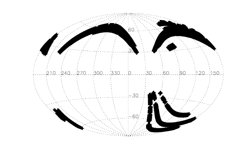
Figure 1: Sky coverage for the SDSS dataset used in this work. The total area covered by our data is $\sim$2500 deg².

We supplemented the SDSS data with data from the RC3 catalog (de Vaucouleurs et al., 1991) for two reasons. First, as we are identifying isolated galaxies (see below), we want to avoid choosing galaxies that have bright neighbors outside the area covered by the SDSS at the time we made our sample; the RC3 provides a catalog of galaxies over the whole sky to make this possible. While it is true that the RC3 catalog is not complete, especially at larger distances, missing companions in the SDSS data are much more likely for the nearest galaxies for which the area on the sky corresponding to our isolation criterion is large. For these, the RC3 catalog should be nearly complete. Another, possibly more important, reason for using the RC3 is that the version of PHOTO that we were using did not provide accurate photometry for large and bright galaxies owing to problems with the deblending algorithm. As a result, we used RC3 $B_{T}$ magnitudes (or photographical magnitudes if $B_{T}$ was not available), corrected for foreground reddening, for all of the SDSS galaxies for which we found a match in the RC3 catalog (within 0.5 arcmin on the sky and 100 km s^-1 in velocity); for all of the other galaxies (which are the smaller galaxies for which the SDSS photometry is accurate), we transformed the SDSS $g$ magnitude to $B$ magnitudes using the relation given by Yasuda et al. (2001).

Our main galaxy list was selected from the full redshift sample by taking all galaxies with $500<cz<60,000~{}\mbox{km~{}s${}^{-1}$}$ and apparent magnitude $r^{\prime}<17.7$; the total number of selected galaxies is 206,352. Distances are derived assuming a smooth Hubble flow with $h=0.7$ ($H_{0}=$ 100 $h^{-1}$ km s^-1 Mpc^-1); the heliocentric velocities were converted to the Local Group Standard of Rest before computing distances.

For the study of satellite dynamics, we define primary galaxies to be those with absolute blue magnitude brighter than $M_{B}=-19.0$. We put no restriction on Hubble type. We use three different isolation and selection criteria to define three different samples of isolated primaries. To be considered as isolated, a galaxy must have no other galaxies within a magnitude difference $\Delta M$, projected separation $\Delta R$, and velocity separation $\Delta V$. Satellites are defined as all objects within a projected distance $\delta r$ and velocity difference $\delta v$ and being at least $\delta m$ magnitudes fainter than the primary. Table 1 gives the parameters used to define each sample, and the number and median distance of primaries, and the number of satellites.

The first two samples have identical isolation criteria, but Sample 2 is defined for primaries out to a larger distance, hence only bright satellites can be seen for the more distant galaxies. The shallower sample has more satellites per primary, but the more distant sample has an overall larger number of total satellites. The third sample mimics conditions used by McKay et al. (2002), in which the isolation criterion is significantly relaxed. It has a very large search radius (almost 3 Mpc), but the luminosity of the neighbors can be quite large: half that of the luminosity of the primary. In other words, this prescription can pick a bright member of a group of galaxies and erroneously treat it as an “isolated” galaxy. As discussed below we obtain similar results for all of the samples, suggesting that our results are statistically significant and do not depend on the exact isolation criterion. Our main results are based on the first two samples.

Table 1: Selection and isolation criteria for SDSS samples

Parameter	Sample 1	Sample 2	Sample 3
Maximum depth of the sample (km s-1)	10,000	60,000	60,000
Constraints on bright neighbors:
Magnitude difference, $\Delta M$	2.0	2.0	0.75
Minimum projected distance, $\Delta R$ ($h^{-1}$ kpc)	500	500	2000
Minimum velocity separation, $\Delta V$ (km s-1)	1000	1000	1000
Constraints on satellites:
Minimum magnitude difference, $\delta m$	2.0	2.0	1.5
Maximum projected distance to primary, $\delta r$ ($h^{-1}$ kpc)	350	350	500
Maximum velocity separation with primary, $\delta v$ (km s-1)	500	500	1000
Number of isolated galaxies	1278	88603	26807
Number of satellites	453	1052	2734
Statistics of isolated galaxies with at least one satellite:
Number	283	716	1107
Mean distance (km s-1)	7100	14700	23170
Mean distance (km s-1) for $-19.5<M_{B}<-20.5$	7244	9785	11076
Mean distance (km s-1) for $-20.5<M_{B}<-21.5$	7697	15917	20854
Limiting magnitude $M_{B}$	$-$16.4	$-$18.0	$-$19.0

Figure 2 shows distributions of primary and satellite brightnesses, brightness ratios, and number of satellites per primary for Sample 1. Considering only primaries for which there is at least one satellite, we find on average two satellites per primary in our first sample, which is similar to that found by Zaritsky et al. (1997) and McKay et al. (2002). A visual morphology classification of our primaries in Sample 1 indicates that about 30% of the galaxies are ellipticals and S0s (E–SO). This fraction of early-type galaxies is simiar as seen in the RC3 catalog and in the SDSS (Nakamura et al., 2002). A fraction of our primaries is close to the edges of the strips and therefore we do not cover their entire halos; for 84$\%$ of the primaries the whole volume is covered.

Given the limiting magnitude of the SDSS spectroscopic survey, we expect to find satellites down to $M_{B}\sim-14$ for a primary with $cz=2000$ km s^-1 and down to $M_{B}\sim-17$ for a primary with $cz=7100$ km s^-1, the mean of our primary recessional velocities in Sample 1. These limits would yield about four satellites per primary for our nearest primaries and 1–2 satellites for the further ones if we assume that all galaxies have satellite luminosity functions similar to that of the Local Group (see Pritchet, & van den Bergh, 1999; Grebel, 2000). Samples 2 and 3 include more distant primaries, and only brighter satellites for the more distant galaxies (see Table 1 for limiting magnitudes).

Figure 2: Statistics of primary galaxies and their satellites in a subsample with velocities less than $10,000~{}\mbox{km~{}s${}^{-1}$}$. The top left panel shows the distribution of absolute blue magnitudes, $M_{B}$, of isolated primaries that have at least one satellite; the top right panel shows the brightnesses of the satellites. The magnitude differences between the primaries and the satellites is presented in the bottom left panel. The number of satellites around each host is shown in the bottom right panel.

The main physical properties of satellites and primaries, such as their color distribution, spectral properties, and their subdivision into early- and late-type galaxies will be discussed in Vitvitska et al. (2003).

3 Numerical models

Cosmological simulations of galactic dark matter satellites in the hierarchical model of structure formation predict a remarkably large number of dark matter satellites orbiting around a Milky Way-size halo (Klypin et al., 1999; Moore et al., 1999). In many respects the simulations are quite realistic; we use them to develop a method for removing the effects of interlopers on the amplitude and shape of the r.m.s. velocity profile of the satellites. Note that the results of the simulations are not used in the reduction of the real astronomical data.

We use one of the simulations presented by Klypin et al. (2001). The simulation is done for the standard $\Lambda$ CDM cosmological model with $\Omega_{0}=0.3$, $\Omega_{\Lambda}=0.7$, and $h=0.7$; the spectrum normalization is $\sigma_{8}=0.9$. The Adaptive-Refinement-Tree (ART) code (see Klypin et al., 2001, for details) is used to run the simulation. The simulation box was $25\ \mbox{$h^{-1}$ Mpc}$. The formal force resolution was $100\ h^{-1}$ pc; the mass resolution is $1.2\times 10^{6}~{}\mbox{$h^{-1}\ M_{\odot}$}$.

The simulation has three galaxy-size halos. All halos are relaxed and have cusps. The outer parts of the density profiles of the halos are well approximated by an NFW profile. The distance between two of the halos is 600 kpc; we decided not to use this pair because the halos are not isolated. We selected the third halo, which does not have a massive companion within 3 Mpc  radius. This halo has a virial mass of $1.5\times 10^{12}\ \mbox{$h^{-1}\ M_{\odot}$}$, a virial radius of 235 $h^{-1}$ kpc, and a maximum circular velocity of 214 km s^-1. There are 200 dark matter satellites inside a 350 $h^{-1}$ kpc  radius from the center of the halo. Most of the satellites are very small with circular velocity of 10–15 km s^-1 and mass $5\times 10^{7}\ \mbox{$h^{-1}\ M_{\odot}$}$.

The simulations were done in such a way that only regions around the three large halos ($\sim$1/2 Mpc) have high resolution. The rest of the computational volume was simulated with significantly lower resolution. No halos outside the regions of high resolution are used in our analysis.

3.1 Satellites in cosmological simulations: removal of interlopers

In any sample of isolated bright galaxies and their satellites there is a fraction of galaxies that are probably not related to the host, but which are included in the sample because of projection effects. We call these objects interlopers. The interlopers tend to have large velocity differences and large projected separations. The fraction of interlopers in the samples of Zaritsky & White (1994) and Zaritsky et al. (1997) was $15\%$. We expect a similar level of contamination in our observational samples. If the interlopers are not removed, the r.m.s. velocity of satellites, and the inferred mass of the primaries, will be overestimated. We use the simulations described in the last section to test prescriptions for removing the interlopers.

Figure 3: The absolute value of the line-of-sight velocity difference between satellites and the central halo as a function of projected distance to a simulated dark matter halo in the standard $\Lambda$ CDM  model. Filled circles show (true) satellites with 3D distance less than 350 $h^{-1}$ kpc  from the central halo with mass $M_{\rm vir}=1.5\times 10^{12}\mbox{$h^{-1}\ M_{\odot}$}$. Open circles show a realization of interlopers, which were generated by randomly placing objects inside a cylinder of radius 350 $h^{-1}$ kpc  and length 1000 km s^-1. The number of interlopers is defined by the luminosity function of galaxies in the SDSS. The dashed curve gives the r.m.s. velocity in the combined sample. The full curve shows the r.m.s. velocity of true satellites.

To understand how interlopers might affect the results we introduce them into the simulation. We have to do this because the $N$-body simulation resolves only the region very close to the central halo; no interlopers are present in the simulation. To make a sample that realistically mimics the observational data we start by making an estimate of the number of expected interlopers in the observed sample. Using the SDSS field luminosity function (Blanton et al., 2001) we find that 0.43 galaxies between $-18<M_{B}<-16$ are expected inside a volume $R<350~{}\mbox{$h^{-1}$ kpc}$ and with a velocity dispersion of $|\Delta V|<500~{}\mbox{km~{}s${}^{-1}$}$ at a distance of $\sim$5000 km s^-1. This is the estimated number of interlopers per primary, if galaxies are randomly distributed in space. Neglecting the large-scale correlations of galaxies appears to be a reasonable assumption at this point, because our primaries are selected to avoid clusters and groups of galaxies. The latter are responsible for most galaxy clustering on a scale of a few megaparsecs. Thus, the clustering of galaxies (with the exception of true satellites) around our primaries is small and can be neglected. Using simulations this point should be quantified in more detail in the future.

In the observed samples we find on average two satellites per primary. Thus, we expect 0.215 interlopers for each true satellite. In our numerical simulation we have 200 true satellites. This means that we expect about 43 interlopers. We randomly place 43 interlopers into a cylinder of radius $R=350~{}\mbox{$h^{-1}$ kpc}$ and length $1000~{}\mbox{km~{}s${}^{-1}$}$.

Figure 3 shows the resulting velocity differences for both satellites and interlopers as a function of projected distance to the parent dark matter halo, as well as the r.m.s. velocities for the true satellites and for the combined sample of the satellites and interlopers. Since the interlopers are not physically associated with the primaries, their number depends only on the volume. Therefore, their effect on the r.m.s. velocity is stronger at larger distances. Neglecting interlopers clearly leads to an apparent increase in the r.m.s. velocity with distance, while the r.m.s. velocity of the true satellites actually decreases with distance.

To reliably estimate the satellite velocity dispersion, one needs to find a way to account for the interlopers. We start by characterizing the velocity distribution of true satellites. Motivated by Figure 3, we consider a Gaussian velocity distribution, but allow the width of the distribution to change with radius. Figure 4 shows the resulting distribution of normalized (to the r.m.s. velocity in different radial bins) velocities, and demonstrates that the distribution is very close to Gaussian. In reality, the distribution cannot be completely Gaussian because satellites with very high velocities will not be bound to the halo, and will escape. Using simple arguments based on the virial theorem, one naively expects that satellites with velocities twice the r.m.s. velocity should not be bound. Indeed, we find an indication of this: in Figure 4 the points are systematically below the Gaussian fit for $\Delta V>2\sigma$. However, it is difficult to use the simple argument because we measure only one component of the velocity and because the escape velocity changes with distance. In any case, the Gaussian fit provides a reasonably accurate approximation for the distribution of the line-of-sight velocities of true satellites.

A simple prescription far removing the interlopers was used by McKay et al. (2002). The velocity difference distribution of the entire sample of neighbors (including objects at all projected distances) was fitted by a Gaussian + constant function. The idea is that the Gaussian describes the velocity distribution of satellites, and that the constant takes into account the distribution of interlopers; the width of the Gaussian component gives a direct measurement of the r.m.s. velocity of the satellites. Our simulations show that the velocities of the true satellites are indeed well approximated by the Gaussian distribution, but that the width of the distribution (i.e., the velocity dispersion) is a function of radius. We find that the McKay et al. (2002) prescription has two problems that result from making a single fit over all radii:

(1) The level of interloper contamination (the constant in the fit) does not depend on the distance to the primary. This is inaccurate because of a purely geometrical factor: the volume and thus, the number of interlopers, is larger for larger radii. Neglecting this dependence produces a bias: the r.m.s. velocity is overestimated at large radii and underestimated at small radii.

(2) There is no allowance for dependence of the velocity dispersion on projected distance. Because this dependence is in fact what we wish to study, we do not want to impose the assumption of a constant velocity dispersion on the prescription for the removal of interlopers.

Figure 4: The distribution of relative velocities of true satellites in $N$-body simulations. The distribution is very close to Gaussian (full curve). The distribution was obtained by finding the r.m.s. velocities for individual bins and then combining the normalized velocities.

In fact, if we apply the McKay et al. (2002) prescription to the simulations, we find that the recovered profile of the (interloper-removed) r.m.s. velocity is flat; the prescription fails to recover the true dispersion profile of the satellites. In this article, we apply an improved interloper prescription by making a separate “Gauss + constant” fit for separate radial bins. In this case the increase of the number of interlopers with the projected distance is taken into account (at least approximately). This also allows for a radially dependent velocity dispersion of true satellites. In practice we use $100~{}\mbox{kpc}$  radial bins (70 $h^{-1}$ kpc  in numerical simulations) and 100 km s^-1  velocity bins. We do not include satellites with projected distance less than $20~{}\mbox{kpc}$. The binned data are used to minimize the sum over all bins of normalized deviations $(V_{i,\rm obs}-V_{i,\rm model})^{2}/N_{i}$, where $N_{i}$ is the number of velocities in the $i$th bin, and $V_{i,\rm obs}$ and $V_{i,\rm model}$ are the observed and modeled velocities in the bin.

Figure 5 shows the accuracy of the recovery of the true r.m.s. velocity for the simulation; the short-dashed line shows the recovered velocity while the solid line shows the true velocity distribution of the satellites. The procedure works remarkably well. It recovers the value of the velocity dispersion and the number of interlopers. In the next section, we apply the same procedure to the observational samples.

The theoretical prediction for the velocity dispersion profile for an NFW profile with the same virial mass as that of the simulated dark matter halo is shown by a long-dashed line. In order to make this prediction for the r.m.s. line-of-sight velocity, we use the NFW profile and assume that the satellites are in equilibrium. We then use the Jeans equation to find the velocity dispersion. The velocity anisotropy $\beta(r)\equiv 1-\sigma_{\perp}^{2}/2\sigma_{r}^{2}$, which is needed for the equation, was taken from cosmological simulations (Colín, Klypin, & Kravtsov, 2000; Vitvitska et al., 2002). (Here $\sigma_{\perp}$ and $\sigma_{r}$ are the tangential and radial r.m.s. velocities). The velocity anisotropy changes from very small values $\beta\approx 0$ close to the center of a halo to $\beta\approx 0.5-0.6$ at the virial radius. We use this dependence of $\beta$ on radius to make analytical estimates of the projected velocity dispersion. Specifically, we integrate the r.m.s. velocities, which we obtain from the Jeans equation, along a line of sight. The integration is truncated at 1.5 virial radii. The velocity anisotropy enters these calculations twice: through the Jeans equation and during the integration along the line of sight. For a fixed mass profile $M(r)$ the effects of the velocity anisotropy are rather mild. The line-of-sight r.m.s. velocity in the realistic non-isotropic halo declines with distance slightly more rapidly as compared with the isotropic case ($\beta=0$).

Figure 5: The same as in Figure 3. The long dashed and dot-dashed curves show respectively the velocity dispersion and the escape velocity for the NFW profile with the same virial mass as the real dark matter halo. Most of the interlopers are above the escape velocity – they cannot possibly belong to the dark matter halo. The r.m.s. velocity of the true satellites is plotted using the solid curve. This r.m.s. velocity of true satellites is accurately recovered (short-dashed curve) from the total sample of satellites + interlopers by making the Gaussian + constant fit for velocities in individual radial bins.

4 Results

4.1 Radial dependence of satellite velocity dispersion

Figure 6: The line-of-sight velocity differences of satellites in SDSS Sample 2 (open circles) for primaries in the range $-19.5<M_{B}<-20.5$. The dashed curve shows the r.m.s. velocities for raw data with no removal of interlopers (except for the $\pm 500~{}\mbox{km~{}s${}^{-1}$}$ cut of the velocities). The r.m.s. velocity is basically flat; it does not depend on the distance to the primary. The full curve shows theoretical prediction for equilibrium NFW halo with mass $\mbox{M${}_{\rm vir}$}=5\times 10^{12}\ \mbox{M${}_{\odot}$}$. The decline in velocities is not observed in the raw data.

Figure 7: The same as in Figure 6, but for Sample 3 with primaries in the range $-20.5<M_{B}<-21.5$. The short dashed curve shows the r.m.s. velocities for raw data; the r.m.s. velocity increases slightly with the distance. The full curve with the error bars shows the r.m.s. velocity after removal of interlopers in each radial bin; the r.m.s. velocity is clearly declining with distance. It is consistent with the NFW prediction (full curve) for halos with virial mass, $\mbox{M${}_{\rm vir}$}=6\times 10^{12}\ \mbox{M${}_{\odot}$}$. The long dashed curve shows the escape velocity from the NFW halo of this mass.

Figure 8: The same as in Figure 6, but with the removal of the interlopers. The full curve with the error bars shows the r.m.s. velocity after removal of interlopers. As in Figure 7, the r.m.s. is clearly declining and consistent with the NFW profile (short-dashed curve) with $\mbox{M${}_{\rm vir}$}=1.5\times 10^{12}\ \mbox{M${}_{\odot}$}$. The long dashed curve shows the escape velocity from the NFW halo of this mass. All satellites above the escape velocity curve are interlopers.

Figure 6 shows the relative line-of-sight velocities for a subset of Sample 2; only companions of galaxies with $-19.5<M_{B}<-20.5$ are shown. Figure 7 shows a comparable plot for Sample 3, but only for the brighter primaries, since the statistics are poor for the fainter primaries. The raw r.m.s. velocity is shown by the dashed curve. Both figures show that the r.m.s. velocity of the raw (uncorrected) data either does not change or slightly increases with the distance from the primary. A few years ago this would have been a strong argument in favor of dark matter in the outer parts of galaxies, but as discussed in the introduction, a flat r.m.s. velocity curve extending to 300 kpc  strongly contradicts any existing dark matter model. Taken at face value, the raw r.m.s. velocities presented in Figures 6 and  7 contradict the dark matter scenario, and actually favor MOND.

However, if we remove interlopers using the Gauss + constant technique discussed in the previous section, as shown by the full lines with error bars in Figures 7 and 8, we find that the velocity dispersion of satellites declines with distance. We note that the results for Sample 1, which extends to fainter satellites, are similar to those shown here for the other two samples. Using Monte Carlo simulations, we reject a hypothesis that the r.m.s. velocity is constant at the 97% level corresponding approximately to the 3$\sigma$ level for Gaussian statistics. For the simulations we combine Samples 2 and 3, which provide independent measurements. We assume that deviations of the r.m.s. velocities are Gaussian in each of four bins for each sample. The average value of the r.m.s. velocity is defined by four random points. The probability of having $\chi^{2}$ larger than the observed $\chi^{2}$ and declining curves in two independent realizations is $2.9\times 10^{-2}$, based on 10,000 realizations. Most of the constraints come from Sample 2, where the first and the last points deviate from the average by 1.5$\sigma$ and 1.8$\sigma$ correspondingly. Sample 3 alone is consistent with the constant r.m.s. velocity. Still, even in this case the velocity declines. When we combine both samples, the constant r.m.s. velocity becomes very improbable.

The number of estimated interlopers is quite modest. For Sample 1, which has 132 satellites for primaries in the range $-19.5<$M_B$<-20.5$, we estimate that 23 are interlopers: 17% of the sample. The numbers are similar for the other samples: 19% in Sample 2 and 20% in sample 3. As expected from geometrical arguments, the number of interlopers increases with the radius. For example, in Sample 3 the number of estimated interlopers is 16.7 for radii in the range 100–200 kpc, and 54 for 200–360 kpc, which is roughly consistent with a constant number of interlopers per unit volume.

The observed decline in velocity dispersion with radius closely matches that predicted by an NFW dark matter density profile. Figures 7 and 8 give the predicted NFW velocities for halos of mass $6\times 10^{12}\ \mbox{M${}_{\odot}$}$ (for primaries with $-20.5<M_{B}<-21.5$) and $M_{\rm vir}=1.5\times 10^{12}\ \mbox{M${}_{\odot}$}$ (for primaries with $-19.5<M_{B}<-20.5$).

If we remove interlopers using the method of McKay et al. (2002), the mean velocity dispersion for each magnitude bin is smaller than the raw value, but we do not get a declining velocity curve. This explains the difference between our conclusions and those of McKay et al. (2002), who do not find a radial dependence on velocity dispersion; as discussed above, we feel that our procedure of allowing for the radial dependence of interloper contamination is better motivated physically.

4.2 Relation of satellite velocity dispersion with host luminosity

A comparison of Figures 7 and 8 clearly indicates that the r.m.s. velocity increases with the luminosity of the primary. This contradicts the earlier results of Zaritsky et al. (1997). Because the NFW profile provides an accurate fit to the observed velocity dispersion profile, we can use it to estimate the virial mass of each group of galaxies. For galaxies with $-19.5<M_{B}<-20.5$ we find $M_{\rm vir}=1.5\times 10^{12}\ \mbox{M${}_{\odot}$}$. For the brighter magnitudes, $-20.5<M_{B}<-21.5$, the virial mass is $M_{\rm vir}=6\times 10^{12}\ \mbox{M${}_{\odot}$}$. These values give us virial mass-to-light ratios $M/L=100$ and $M/L=150$ for the dimmer and brighter galaxies correspondingly. Thus, the $M/L$ ratio increases with the luminosity roughly as $M/L\approx L^{0.5}$. We believe that this change in $M/L$ with luminosity is real and does not reflect a change in the stellar populations for both magnitude bins. A reason for this is that we did not see a dependence of the fraction of E–S0 with luminosity for the primaries in Sample 1, at least from $-$19 to $-$22 blue absolute magnitudes. A similar increase of $M/L$ with luminosity ($M/L\propto L^{0.4\pm 0.2}$) has been seen from weak lensing studies by Guzik & Seljak (2002). See, however, McKay et al. (2001) who, also from weak lensing, found no dependence of the $M/L$ on luminosity.

Instead of trying to estimate masses of the galaxies (which is bound to be model-dependent), we can study the more direct dependence of the r.m.s. velocity on the luminosity of the primary galaxy. This can be viewed as an analog of the Tully–Fisher relation. Figure 9 presents the dependence of the satellite r.m.s. velocity, computed within 120 kpc as a function of galaxy luminosity. We calculate the r.m.s. velocity relatively close to the primary galaxy because within this distance the velocity dispersion depends only weakly on the distance to the primary for all primaries considered here. Hence, we can meaningfully compare results from galaxies that might have different sizes. The estimated value of the velocity dispersion for an $L_{*}$ galaxy from weak lensing studies (Hoeskstra, Yee, & Gladders, 2001; McKay et al., 2001) is also shown; the results of lensing studies are very close to those derived from the SDSS satellite data.

The results are consistent with a slope of $\sigma\propto L^{0.3}$. We can write this dependence using a form analogous to the Tully–Fisher relation:

$$M_{B}=0.02-8.7\log(2\sigma).$$ (1)

This relation is shown in Figure 9. The slope of this relation is the same as for spiral galaxies (Verheijen, 2001), which is shown as a long-dashed line in the figure. The zero point for the spiral relation was shifted down by factor of 1.6 to match the SDSS data points; this factor is close to the naively expected $\sqrt{3}$ correction from rotational velocity to 1D line-of-sight velocity. The remaining difference of 8% is difficult to assign to any particular effect; there are several effects that could produce the small difference (e.g., projection effects, and non-isotropic orbits).

However, when we compute the r.m.s. velocity within a larger radius of 350 kpc, we find $\sigma\propto L^{0.5}$. The reason for the steeper slope is a combination of the very large radius and declining $\sigma(r)$, which will occur if the density profiles of halos at different mass are not homologous, e.g., if the concentration of the halo decreases with increasing mass. This is consistent with theoretical prediction.

It is rather straightforward to find the $\sigma$–virial mass relation for the NFW halos. Using the model described in Section 3.1 (equilibrium NFW with slightly anisotropic velocities), we find the line-of-sight r.m.s. velocity averaged for radii 20–100 kpc and the line-of-sight velocity for projected distance 350 kpc. The results are shown in Figure 10. For the range of masses considered here, the $\sigma$–$M$ relations are power laws. Just as the observed slope of the $\sigma$–$L$ relation, the slope of the $\sigma$–$M_{\rm vir}$ relation increases with the radius within which the r.m.s. velocity is calculated. For the 350 kpc  radius the slope 0.5 is the same as the slope of the $\sigma$–$L$ relation for the same radius. This would imply a constant mass-to-light ratio. This result, being formally correct, is a bit misleading. Measured in terms of a more physically motivated quantity, the virial radius, the $M/L$ ratio increases with luminosity.

Comparison with theoretical predictions of the luminosities is more complicated and will be deferred to another paper. We use only the virial $M/L$ for two magnitudes $M_{B}=-20$ and $-21$. In a recent paper, Yang et al. (2002) ask which model parameters are required for the cosmological models to explain the observed luminosity function and the Tully–Fisher relation. The main uncertainty is the $M/L$ ratio. Yang et al. (2002) predict an $M/L(L)$ that is needed to account for observations. We compare our two $M/L$ ratios with the Yang et al. (2002) predictions and find them remarkably close. However, this comparison actually required numerous corrections, including a correction for overdensity of 180 to the virial overdensity, correction for galactic absorption, correction for different bands, and scaling with the Hubble constant. The corrections were provided by Rachel Somerville. Preliminary comparison with semi-analytical models (Somerville, private communication) indicate a problem: observed galaxies are $\approx$0.75 mag too bright as compared with theoretical predictions.

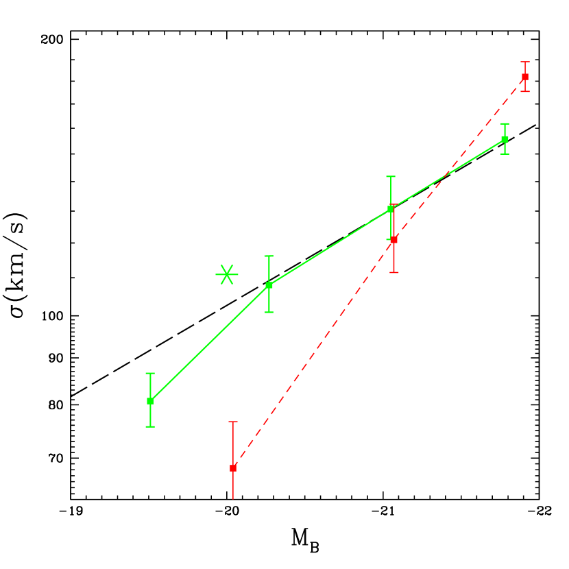
Figure 9: The dependence of satellite r.m.s. velocity on the absolute $B$ magnitude of the primary galaxy. The solid line shows r.m.s. velocity inside 120 kpc. The long-dashed line shows the Tully–Fisher relation of spiral galaxies (Verheijen, 2001) scaled down by a factor of 1.6 to account for the difference in definitions of velocities. The short-dashed line shows the r.m.s. velocity for satellites in the outer radial shell 250–350 kpc. For these large radii the r.m.s. velocity is consistent with $\sigma\propto L^{0.5}$ (constant $M/L$). The asterisk shows the weak lensing results for $L_{*}$ galaxies (Hoeskstra, Yee, & Gladders, 2001)

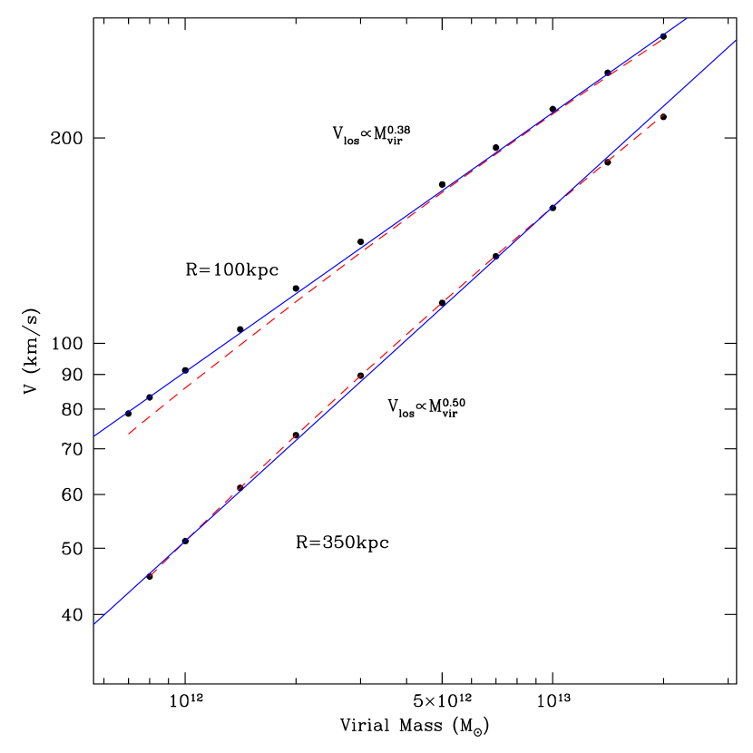
Figure 10: Theoretical predictions for the line-of-sight r.m.s. velocity, $\sigma$, at different projected distances as the function of galaxy virial mass. The dots show the velocities for equilibrium NFW halos. The top curves and symbols are for velocities averaged for radii 20–100 kpc. The bottom curves are for projected distance 350 kpc. Power-law fits indicated in the plot with full lines provide very accurate approximations. The dashed curves are 1D tangential r.m.s. velocity at 100 kpc and at 350 kpc.

5 Conclusions

We construct samples of isolated galaxies and associated satellites using data from the SDSS. We detect about 3000 satellites with absolute blue magnitudes going down to $M_{B}=-14$. Analysis of the satellite velocities clearly indicates that galaxies are embedded in large halos extending to distances up to $350~{}\mbox{kpc}$. Our measured velocity dispersion for $\sim L_{*}$ galaxies is in agreement with measurements from weak lensing studies.

Our analysis of galaxies selected from the SDSS database clearly indicates that the line-of-sight r.m.s. velocity of satellites declines with the distance to the primary galaxy. Similar results were found for each of our three samples, suggesting that it is robust to statistical effects and the exact definition of an isolated galaxy. This decline agrees remarkably well with $\rho\propto r^{-3}$ predicted by all cosmological models. Both the isothermal and MOND profiles contradict the observational results. Observations of weak lensing from the SDSS combined with the Tully–Fisher and Fundamental Plane relations (Seljak, 2002) also finds that the galactic halo profiles has to be steeper than isothermal at large radii.

Interlopers play an important role. We believe that the decline in satellite velocity was not seen previously (Zaritsky & White, 1994; Zaritsky et al., 1997; McKay et al., 2002), mainly because of either lack of statistics or insufficient removal of interlopers. We use numerical simulations to test prescriptions for correcting the effects of interlopers and isolation criteria. Both effects – interlopers and isolation criteria – have a tendency to overestimate of the mass of the dark matter halo and imply a velocity profile that is too flat.

We find that the satellite velocity dispersion inside a projected 100 kpc radius and the absolute blue magnitude of the galaxy are related as $M=0.02-8.7\log(2\sigma)$ ($\sigma\propto L^{0.3}$). This dependence is in agreement with the slope and the zero point of the Tully–Fisher relation for spiral disks. If we calculate the r.m.s. velocity within a radius of $350~{}\mbox{kpc}$, the slope of the velocity–luminosity relation is visibly steeper: $\sigma\propto L^{0.5}$. The likely explanation for the difference in the slopes is an interplay between the shape of the velocity dispersion and the virial radius of galaxies.

The mass-to-light ratio increases with luminosity as $M/L\propto L^{0.5}$. For $M_{B}=-20$ (-21) we find that the virial $M/L=100$ (150).

References

- Avila-Reese et al. (2001) Avila-Reese, V., Colín, P., Valenzuela, O., D’Onghia, E., & Firmani, C. 2001, ApJ, 559, 516
- Blanton et al. (2001) Blanton, M. R. et al. 2001, AJ, 121, 2358
- Blanton et al. (2002) Blanton, M. R., Lupton, R. H., Maley, F. M., Young, N., Zehavi, I., & Loveday, J. 2002, AJ, submitted, astro-ph/0105535
- Bosma (1981) Bosma, A. 1981, AJ, 86, 1825
- Brainerd, Blandford, & Smail (1996) Brainerd, T. G., Blandford, R. D., & Smail, I. 1996, ApJ, 466, 623
- Buote & Canizares (1994) Buote, D. A. & Canizares, C. R. 1994, ApJ, 427, 86
- Buote et al. (2002) Buote, D. A., Jeltema, T. E., Canizares, C. R., & Garmire, G. P. 2002, ApJ, 577, 183
- Colín et al. (2000) Colín, P., Avila-Reese, V., Valenzuela, O., & Firmani, C. 2002, astro-ph/0205322
- Colín, Klypin, & Kravtsov (2000) Colín, P., Klypin, A. A., & Kravtsov, A. V. 2000, ApJ, 539, 561
- de Vaucouleurs et al. (1991) de Vaucouleurs et al. 1991, “Third Reference Catalogue of Bright Galaxies”, University of Texas Press, Austin
- Erickson, Gottesman, & Hunter (1987) Erickson, L. K., Gottesman, S. T., & Hunter, J. H. 1987, Nature, 325, 779
- Evans & Wilkinson (2000) Evans, N. W. & Wilkinson, M. I. 2000, MNRAS, 316, 929
- Evans et al. (2000) Evans, N. W., Wilkinson, M. I., Guhathakurta, P., Grebel, E. K., & Vogt, S. S. 2000, ApJ, 540, L9
- Faber & Gallagher (1979) Faber, S. M. & Gallagher, J. S. 1979, ARA&A, 17, 135
- Fischer et al. (2000) Fischer, P. et al. 2000, AJ, 120, 1198
- Fukugita et. al. (1996) Fukugita, M., Ichikawa, T., Gunn, J. E., Doi, M., Shimasaku, K., & Schneider, D. P. 1996, AJ, 111, 1748
- Ghigna et al. (2000) Ghigna, S., Moore, B., Governato, F., Lake, G., Quinn, T., & Stadel, J. 2000, ApJ, 544, 616
- Grebel (2000) Grebel, E. K. 2000, Star formation from the small to the large scale. Proceedings of the 33rd ESLAB symposium on star formation from the small to the large scale. Edited by F. Favata, A. Kaas, and A. Wilson. ESTEC, Noordwijk, The Netherlands. ESA SP 445., p.87
- Gunn et al. (1998) Gunn, J. E. et al. 1998, AJ, 116, 3040
- Guzik & Seljak (2002) Guzik, J. & Seljak, U. 2002, MNRAS, 335, 311
- Hoeskstra, Yee, & Gladders (2001) Hoeskstra, H., Yee, H. K. C., & Gladders, M. D. 2001, proceedings for ”Where’s the matter? Tracing dark and and bright matter with the new generation of large scale surveys”, Marseille, 2001, astro-ph/0109514
- Hogg et. al. (2001) Hogg, D. W., Schlegel, D. J., Finkbeiner, D. P., & Gunn, J. E. 2001, AJ, 122, 2129
- Kauffmann et al. (1999) Kauffmann, G., Colberg, J. M., Diaferio, A., & White, S. D. M. 1999, MNRAS, 303, 188
- Keeton (2001) Keeton, C. R. 2001, ApJ, 561, 46
- Keeton, Kochanek, & Falco (1998) Keeton, C. R., Kochanek, C. S., & Falco, E. E. 1998, ApJ, 509, 561
- Klypin et al. (2001) Klypin, A., Kravtsov, A. V., Bullock, J. S., Primack, J. R., 2001, ApJ, 554, 903
- Klypin et al. (1999) Klypin, A., Kravtsov, A. V., Valenzuela, O., & Prada, F. 1999, ApJ, 522, 82
- Kochanek (1996) Kochanek, C. S. 1996, ApJ, 457, 228
- Lin, Jones, & Klemola (1995) Lin, D. N. C., Jones, B. F., & Klemola, A. R. 1995, ApJ, 439, 652
- Lupton et al. (2001) Lupton, R., Gunn, J. E., Ivezic, Z., Knapp, G. R., Kent, S., & Yasuda, N. 2001, in ASP Conf. Ser. 238, Astronomical Data Analysis Software and Systems X, ed. F. R. Harnden, Jr., F. A. Primini, & H. E. Payne (San Francisco: ASP), 269
- McKay et al. (2001) McKay, T. A. et al. 2001. submitted to ApJ, astro-ph/0108013
- McKay et al. (2002) McKay, T. A. et al. 2002, ApJ, 571, L85
- Maller et al. (2000) Maller, A. H., Simard, L., Guhathakurta, P., Hjorth, J., Jaunsen, A. O., Flores, R. A., & Primack, J. R. 2000, ApJ, 533, 194
- Moore et al. (1999) Moore, B., Ghigna, S., Governato, F., Lake, G., Quinn, T., Stadel, J., & Tozzi, P. 1999, ApJ, 524, L19
- Nakamura et al. (2002) Nakamura, O. et al. 2002, astro-ph/0212405
- Navarro, Frenk, & White (1997) Navarro,J. F., Frenk, C. S., & White, S. D. M. 1997, ApJ, 490, 493
- Ostriker, Peebles, & Yahil (1974) Ostriker, J. P., Peebles, P. J. E., & Yahil, A. 1974, ApJ, 193, L1
- Pier et al. (2002) Pier, J. R., Munn, J. A., Hindsley, R. B., Hennessy, G. S., Kent, S. M., Lupton, R. H., & Ivezic, Z. 2002, AJ, submitted
- Pritchet, & van den Bergh (1999) Pritchet, C. J. & van den Bergh, S. 1999, AJ, 118, 883
- Roberts & Rots (1973) Roberts, M. S. & Rots, A. H. 1973, A&A, 26, 483
- Romanowsky & Kochanek (1998) Romanowsky, A. J. & Kochanek, C. S. 1998, ApJ, 493, 641
- Sancisi & van Albada (1987) Sancisi, R. & van Albada, T. S. 1987, IAU Symp. 117: Dark matter in the universe, 117, 67
- Schlegel, Finkbeiner, & Davis (1998) Schlegel, D. J., Finkbeiner, D. P., & Davis, M. 1998, ApJ, 500, 525
- Schneider & Rix (1997) Schneider, P. & Rix, H. 1997, ApJ, 474, 25
- Seljak (2002) Seljak, U. 2002, MNRAS, 334, 797
- Smith et al. (2001) Smith, D. R., Bernstein, G. M., Fischer, P., & Jarvis, M. 2001, ApJ, 551, 643
- Smith et al. (2002) Smith, J. A., Tucker, D. L., Kent, S. M., et al. 2002, AJ, 123, 2121
- Sofue & Rubin (2001) Sofue, Y. & Rubin, V. 2001, ARA&A, 39, 137
- Stoughton et al. (2002) Stoughton, C. et al. 2002, AJ, 123, 485
- Strauss et al. (2002) Strauss, M. A. et al. 2002, AJ, 124, 1810
- Tyson et al. (1984) Tyson, J. A., Valdes, F., Jarvis, J. F., & Mills, A. P. 1984, ApJ, 281, L59
- van Albada et al. (1985) van Albada, T. S., Bahcall, J. N., Begeman, K., & Sancisi, R. 1985, ApJ, 295, 305
- Verheijen (2001) Verheijen, M. A. W. 2001, ApJ, 563, 694
- Vitvitska et al. (2002) Vitvitska, M., Klypin, A., Kravtsov, A.V., Wechsler, R.H., Primack, J.R., Bullock, J.S. 2002, ApJ, accepted, astro-ph/0105349.
- Vitvitska et al. (2003) Vitvitska, M., Prada, F., Klypin, A., Holtzman, J. et al. 2003, in preparation
- Yang et al. (2002) Yang, X., Mo, H. J., & van den Bosch, F. C., 2002, astro-ph/0207019
- Yasuda et al. (2001) Yasuda, N. et al. 2001, AJ, 122, 1104
- York et al. (2000) York, D.G. et al. 2000, AJ, 120, 1579
- Zaritsky (1992) Zaritsky, D. 1992, ApJ, 400, 74
- Zaritsky et al. (1989) Zaritsky, D., Olszewski, E. W., Schommer, R. A., Peterson, R. C., & Aaronson, M. 1989, ApJ, 345, 759
- Zaritsky et al. (1993) Zaritsky, D., Smith, R., Frenk, C., & White, S. D. M. 1993, ApJ, 405, 464
- Zaritsky et al. (1997) Zaritsky, D., Smith, R., Frenk, C., & White, S. D. M. 1997, ApJ, 478, 39
- Zaritsky & White (1994) Zaritsky, D. & White, S. D. M. 1994, ApJ, 435, 599