The spin periods of magnetic cataclysmic variables
Abstract
We have used a model of magnetic accretion to investigate the rotational equilibria of magnetic cataclysmic variables (mCVs). This has enabled us to derive a set of equilibrium spin periods as a function of orbital period and magnetic moment which we use to estimate the magnetic moments of all known intermediate polars. We further show how these equilibrium spin periods relate to the polar synchronisation condition and use these results to calculate the theoretical histogram describing the distribution of magnetic CVs as a function of . We demonstrate that this is in remarkable agreement with the observed distribution assuming that the number of systems as a function of white dwarf magnetic moment is distributed according to .
Department of Physics and Astronomy, The Open University, Walton Hall, Milton Keynes MK7 6AA, U.K.
Department of Physics and Astronomy, The University of Leicester, University Road, Leicester LE1 7RH, U.K.
1. The sample of mCVs
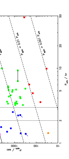
As shown in Figure 1, the mCVs occupy a wide range of parameter space in the spin period () versus orbital period () plane. This indicates that accretion occurs by a variety of different types of magnetically controlled flow. However, certain regions of the diagram are sparsely populated. In order to understand this distribution we use a model of magnetic accretion to investigate the rotational equilibria of these systems. First we discuss the systems included in Figure 1 and their characteristics.
1.1. Synchronous polars
We include 67 synchronous polars ranging from CV Hyi with a period of 77.8 min to V1309 Ori with a period of 7.98 hr. Magnetic field strength estimates exist for 52 of these, spanning the range G cm3. It is apparent that a true period gap no longer exists for polars, however we note that there are 22 synchronous systems with hr and a further 45 systems with hr.
1.2. Asynchronous polars
There are 5 systems in which and differ by around 2% or less. These are assumed to be polars that have been disturbed from synchronism by a recent nova explosion. The systems are V1432 Aql with (Friedrich et al 1996), BY Cam with (Silber et al 1992), V1500 Cyg with (Schmidt & Stockman 1991), V4633 Sgr with (Lipkin et al 2001), and CD Ind with (Schwope et al 1997). In Figure 1 these systems are essentially indistinguishable from the synchronous polars.
1.3. Nearly synchronous intermediate polars
Slightly further away from synchronism than the asynchronous polars are 4 recently discovered systems that may best be described as nearly synchronous intermediate polars. The systems are V381 Vel with (Tovmassian, these proceedings), RXJ0524+42 with (Schwarz, these proceedings), HS0922+1333 with (Tovmassian, these proceedings) and V697 Sco with (Warner & Woudt 2002). Two of these systems lie in the ‘period gap’. We suggest that all four systems are intermediate polars in the process of attaining synchronism and evolving into polars.
1.4. Conventional intermediate polars
We include 22 systems that we classify as conventional intermediate polars. These all have spin to orbital period ratios in the range and hr. The systems are V709 Cas (Norton et al 1999), 1RXSJ154814.5–452845 (Haberl, Motch & Zickgraf 2002), 2236+0052 (Woudt & Warner, these proceedings), V405 Aur (Allan et al 1996), YY Dra (Haswell et al 1997), PQ Gem (Duck et al 1994), V1223 Sgr (Taylor et al 1997), AO Psc (Taylor et al 1997), HZ Pup (Abbott & Shafter 1997), UU Col (Burwitz et al 1996), FO Aqr (de Martino et al 1999), V2400 Oph (Buckley et al 1997), BG CMi (de Martino et al 1995), TX Col (Norton et al 1997), 1WGA1958.2+3232 (Norton et al 2002), TV Col (Vrtilek et al 1996), AP Cru (Woudt & Warner 2002), V1062 Tau (Hellier, Beardmore & Mukai 2002), LS Peg (Rodriguez-Gil et al 2001), RR Cha (Woudt & Warner 2002), RXJ0944.5+0357 (Woudt & Warner, these proceedings), and V1425 Aql (Retter, Leibowitz & Kovo-Kariti 1998). The orbital period of 1RXSJ154814.5–452845 is currently uncertain, and the two possible values are both shown in Figure 1, connected by a horizontal line.
1.5. EX Hya-like systems
There are a further 4 intermediate polars that lie below the ‘period gap’. These all have and hr. Given their location on the versus diagram, we refer to these as ‘EX Hya-like’ systems for convenience. The systems are HT Cam (Kemp et al 2002), RXJ1039.7–0507 (Woudt & Warner 2003a), V1025 Cen (Hellier, Wynn & Buckley 2002) and EX Hya (Allan, Hellier & Beardmore 1998). The systems DD Cir (Woudt & Warner 2003b) and V795 Her (Rodriguez-Gil et al 2002) lie within the ‘period gap’ with and may be included with these systems.
1.6. RXJ1914.4+2456 and RXJ0806.3+1527
RXJ1914 (a.k.a. V407 Vul) and RXJ0806 are X-ray sources that each display a single coherent periodiocity at 569s and 321s respectively. They have been suggested to be double degenerate systems, where the modulation represents the orbital period of either a polar, an Algol-like system or an electrically powered star (Cropper et al 1998, these proceedings; Ramsay et al 2000, 2002a, 2002b; Marsh & Steeghs 2002; Wu et al 2002; Israel et al 1999, 2002, these proceedings). It has also been suggested that the systems are face-on stream-fed intermediate polars (Norton, Haswell & Wynn 2002), in which case the periods observed are beat periods between the white dwarf spin and orbital periods caused by the accretion stream flipping from one pole to the other twice in each synodic period. For stream-fed flow, the orbital periods must be h for RXJ1914 and h for RXJ0806. We include these systems in Figure 1 under the assumption that they are intermediate polars. Their data points are shown with ‘tails’ indicating the upper limits on their spin and orbital periods.
1.7. Rapid rotators
Finally there are a mixed bag of 6 objects that are characterized by rapidly rotating white dwarfs. They all lie in the region of the diagram defined by , but with a large range of orbital periods. They include the very long outburst interval SU UMa star, WZ Sge (Patterson et al 1998) with a proposed spin period of 28 s, the propeller system AE Aqr (Choi, Dotani & Agrawal 1999) with a 33 s spin period, the ‘DQ Her systems’ V533 Her (Thorstensen & Taylor 2000) and DQ Her (Zhang et al 1995), and also XY Ari (Hellier, Mukai & Beardmore 1997) and the long orbital period old nova GK Per (Morales-Rueda, Still & Roche 1996).
2. Spin equilibria
The spin rate of a magnetic white dwarf accreting via a disc reaches equilibrium when the rate of angular momentum accreted by the white dwarf is equal to the braking effect of the magnetic torque on the disc close to its inner edge. The inner edge of such a disc may then be defined as the point where the magnetic stresses exceed the viscous stresses.
Most models for this equilibrium spin period find that the inner edge of the disc, at radius , is roughly equal to the magnetospheric radius and also to the corotation radius, , that is the radius at which a particle in a Keplerian orbit would orbit the white dwarf at the same rate as the white dwarf spins on its axis. This implies that systems whose white dwarfs have low surface magnetic moments will be rapid rotators, whilst systems whose white dwarfs have high surface magnetic moments will be slow rotators.
In turn, this leads to the requirement for truncated accretion disc formation of (i.e. the circularisation radius at which material would first go into orbit around the white dwarf). With this hierarchy of radii, the spin and orbital periods of the system must then satisfy . Whilst this condition is clearly satisfied for the rapid rotators like DQ Her, V533 Her, XY Ari and GK Per, it is clearly not true for all intermediate polars.
Indeed, systems with are unlikely to possess discs, since this implies . King & Wynn (1999) showed that the spin period of EX Hya can be understood as an equilibrium situation in which the magnetospheric and corotation radii extend out to the inner Lagrangian point, . They used simulations of the accretion flow for parameters appropriate to EX Hya to show that a range of equilibrium spin periods are possible, but that the maximum possible spin to orbital period ratio is , in remarkable agreement with the periods of EX Hya. King & Wynn further suggested that a continuum of spin equilibria should exist appropriate to a range of magnetic moments and orbital periods. The aim of the work reported below was to explore this parameter space.
3. The magnetic model
The equation of motion of plasma in a magnetic field is
| (1) |
If we assume the tension term is the dominant force, then the magnetic acceleration is given by
| (2) |
This in turn may be parameterized by introducing the drag parameter via
| (3) |
where is the angular speed of the material orbiting the white dwarf with Keplerian velocity and is the angular speed of the magnetic field lines.
Up to this point, the model is appropriate for any form of magnetic interaction. However, if we now assume that the accertion flow takes the form of diamagnetic blobs, we may express in terms of the magnetic timescale or the magnetic field strength , the Alfvén speed , and the blob density and length .
| (4) |
The blob density is approximated by
| (5) |
and the blob length by
| (6) |
where the sound speed is
| (7) |
with K.
The model outlined above is implemented in a computer code and may be used to allow systems to evolve to their rotational equilibrium. Other examples of the use of the model are presented in King & Wynn (1999), Hellier, Wynn & Buckley (2002) and Ultchin, Regev & Wynn (2002).
4. Results
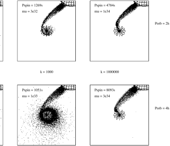
The results of running the model to establish the allowed range of equilibrium spin periods are shown in Figure 2, and Figure 3 shows some example accretion flows corresponding to different regions of the parameter space explored. The model was run for 10 different orbital periods (80 m, 2 h, 3 h, … 10 h) for each of 11 different values of the parameter. These values have been converted into the corresponding value of the white dwarf surface magnetic moment , assuming the diamagnetic blob prescription of Equation 4. Lines on Figure 2 connect the points for each orbital period. The line for an orbital period of 80 m essentially reproduces that obtained by King & Wynn appropriate to EX Hya. It should be noted that there is some latitude in applying the conversion from to (mostly from the assumed values of and describing the blobs), so the envelope of equilibrium periods may shift laterally in the plane. Also, the calculations were performed for a single value of white dwarf mass (0.7 M⊙) and different values will shift the results slightly in the vertical direction. Nonetheless it is encouraging that the predicted equilibrium spin periods lie in the range at which many mCVs are seen. It should also be noted that the estimated magnetic field strengths for the intermediate polars that display polarized emission (e.g. PQ Gem, BG CMi, V2400 Oph and LS Peg) lie within the region covered by the results.
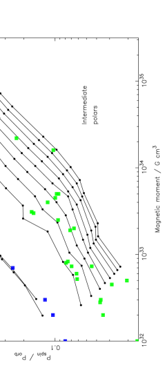
In the envelope of allowed parameter space shown on Figure 2, we note that the region with corresponds to and so indicates regions where truncated accretion discs may form. The region with corresponds to and the region with corresponds to .
If we now assume that all mCVs are at their equilibrium spin period we can place the intermediate polars on Figure 2 by tracing across at the appropriate value to intersect the equilibrium line for the appropriate orbital period. In this way, most of the squares have been placed on Figure 2. For the few systems that have (i.e. EX Hya and the 4 nearly synchronous intermediate polars) we have simply placed them above the mid-point of the plateau part of the relevant curves at the appropriate value. We note that in cases where is measured for intermediate polars, several are spinning up whilst a similar number are spinning down, and FO Aqr has been seen to do both. Hence the assumption that intermediate polars are close to their equilibrium spin periods is a good one with only small deviations apparent on short timescales.
5. Synchronisation
We now use the results obtained above to investigate the polar synchronisation condition. We may assume that systems become synchronized once the magnetic locking torque is equal to the accretion torque. Hence
| (8) |
where the surface magnetic moment on the secondary may be approximated by
| (9) |
from Warner (1996) with in hours. The magnetospheric radius is approximated by the corotation radius,
| (10) |
and the mass accretion rate is set to the secular value given by
| (11) |
for h (McDermott & Taam 1989) and
| (12) |
for angular momemtum loss by gravitational radiation (Warner 1995) which we assume to be dominant at h. The mass ratio is where we assume a primary mass of M⊙ and a secondary mass given by M⊙.
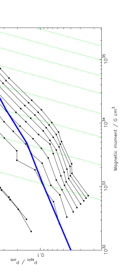
Solutions to Equation 8 are plotted as diagonal lines on Figure 4. Each line connects points at which synchronisation will occur for a given orbital period. The lines shown are for orbital periods of 3 h, 4 h, … 10 h, as those for shorter orbital periods lie to the upper left of the region plotted. Where these diagonal lines intersect the equilibrium spin period lines for their respective orbital periods, gives the points at which systems will synchronize. The locus of these points is shown by the thick line which simply connects the various intersection points. Hence, systems lying below the thick line will not be prone to synchronise, whilst those lying above will tend to do so.
6. Predictions
From Figures 2 and 4 it can be seen that the intermediate polars above the period gap virtually all lie below the sychronisation line. The two systems just above the line are RR Cha and RXJ0944.5+0357 with of 0.161 and 0.168 respectively. We suggest these three are probably normal intermediate polars and within the errors of our calculation are consistent with sitting below the synchronisation line. Lying well above the synchronisation line are the two nearly synchronous intermediate polars V697 Sco and HS0922+1333 with of 0.737 and 0.882 respectively. We suggest that these two systems are on their way to synchronism. A similar fate should hold for the rest of the intermediate polars above the period gap that have relatively high white dwarf magnetic moments.
At short orbital periods, the picture is rather different. All 6 of the EX Hya-like intermediate polars, plus the two nearly synchronous intermediate polars RXJ0524+42 and V381Vel, lie above the synchronisation line and so should be synchronised. We suggest the reason for them not being synchronised could be that the secondary stars in the EX Hya-like systems have low magnetic moments (i.e. less than predicted by Equation 9) and so are unable to come into synchronism.
It is also apparent from Figure 2 that virtually all the intermediate polars have G cm3 whereas virtually all of the polars have G cm3. This discrepancy between the intermediate polar and polar magnetic fields has been noted in the past, and poses the question: where are the synchronous systems with low white dwarf magnetic moments? We can suggest three possibilities for the answer.
Firstly, it may be that the systems with a low white dwarf magnetic moment do synchronize, but in the synchronous state they are primarily EUV emitters and so unobservable. Alternatively it may be that when systems with low white dwarf magnetic moment evolve to short orbital periods, for some reason they simply do not synchronize, but remain on the spin equilibrium line where the rest of the EX Hya-like systems reside. Finally there is the possibility raised by Cummings (these proceedings) that the magnetic fields in intermediate polars are buried by their high accretion rate and so are not really as low as they appear. In this picture, one could envisage that as intermediate polars evolve towards shorter orbital periods, when they reach the period gap the mass transfer shuts off, the magnetic field of the white dwarf re-surfaces, and the systems synchronize before re-appearing below the period gap as conventional, high field, polars.
7. The magnetic moment distribution of white dwarfs in mCVs
The results shown in Figure 4 can also be used to characterize the theoretical distribution of mCVs as a function of the white dwarf surface magnetic moment. We assume that the number of systems varies according to
| (13) |
where is a number to be determined. We may integrate under the equilibrium curves shown in Figure 4 to get the predicted number of systems within a given range of . The number in a given bin is then
| (14) |
where is the gradient of a cubic fit to each of the equilibrium curves in Figure 4. The range of spin to orbital period ratios was divided into eight logarithmic bins, seven of which were 0.25 wide in log space and the eighth corresponded to synchronous systems. The integration was carried out over the magnetic moment range and at the spin to orbital period ratio (for a given orbital period) indicated by the thick line in Figure 4, we assume that systems become synchronized. The predicted number of systems was averaged over orbital periods of 3, 4, 5, and 6 hours assuming systems to be distributed evenly in orbital period, and the final result was normalised to the number of known mCVs with orbital periods greater than 3 h.
The best fit value of the power law index was found to be at 1.95, with a reduced chi-squared of , as shown in Figure 5, although values between 1.85 and 2.05 are also valid (). The cumulative histograms comparing the observed number of systems with that predicted by Equation 13 with is shown in Figure 6, and Table 1.

| Lower edge of bin | |||
|---|---|---|---|
| log() | (obs) | (model) | |
| –2.00 | 0.010 | 1 | 0.00 |
| –1.75 | 0.018 | 1 | 0.00 |
| –1.50 | 0.032 | 4 | 6.19 |
| –1.25 | 0.056 | 11 | 14.08 |
| –1.00 | 0.100 | 4 | 1.21 |
| –0.75 | 0.178 | 1 | 0.08 |
| –0.50 | 0.316 | 0 | 0.00 |
| –0.25 | 0.562 | 2 | 0.00 |
| 0.00 | 1.000 | 26 | 28.45 |

8. Conclusions
We have demonstrated that there is a range of parameter space in the versus plane at which spin equilibrium occurs for mCVs. Using the results of numerical simulations we can infer the surface magnetic moments of the white dwarfs in intermediate polars to be mostly in the range . Most of the intermediate polars with orbital periods greater than 3 h lie below the synchronisation line, whilst most systems with orbital periods less than 2 h lie above it and should be synchronized. High magnetic moment intermediate polars at long orbital periods will evolve into polars. Low magnetic moment intermediate polars at long orbital periods will either: evolve into EX Hya-like systems at short orbital periods; evolve into low field strength polars which are (presumably) unobservable, and possibly EUV emitters; or, if their fields are buried by high accretion rates, evolve into conventional polars once their magnetic fields re-surface when mass accretion turns off. EX Hya-like systems may have low magnetic field strength secondaries and so avoid synchronisation.
We have also shown that the distribution of mCVs above the period gap follows the relationship . Recent data from G. Schmidt (private communication), concerning the magnetic field strength distribution of isolated white dwarfs, reveals a drop off in the number at high magnetic field strengths in those systems too.
References
Abbott, T.M.C., & Shafter, A.W., 1997, ASP Conf. Ser. 121, 679
Allan, A., Horne, K., Hellier, C., Mukai, K., Barwig, H., Bennie, P.J., & Hilditch, R.W., 1996, MNRAS, 279, 1345
Allan, A., Hellier, C., & Beardmore, A.P., 1998, MNRAS, 295, 167
Buckley, D.A.H., Haberl, F., Motch, C., Pollard, K., Schwarzenberg-Czerny, A., & Sekiguchi, K., 1997, MNRAS, 287, 117
Burwitz, V., Reinsch, K., Beuermann, K., & Thomas, H.C., 1996, A&A, 310, L25
Choi, C.S., Dotani, T., & Agrawal, P.C., 1999, ApJ, 525, 399
Cropper, M., 2003, these proceedings
Cropper, M., Harrop-Allin, M.K., Mason, K.O., Mittaz, J.P.D., Potter, S.B., & Ramsay, G. 1998, MNRAS, 293, L57
Cummings, A., 2003, these proceedings
de Martino, D., Mouchet, M., Bonnet-Bidaud, J.M., Vio, R., Rosen, S.R., Mukai, K., Augusteijn, T., & Garlick, M.A., 1995, A&A, 298, 849
de Martino, D., Silvotti, R., Buckley, D.A.H., Gänsicke, B., Mouchet, M., Mukai, K., & Rosen, S.R., 1999, A&A, 350, 517
Duck, S.R., Rosen, S.R., Ponman, T.J., Norton, A.J., Watson, M.G., & Mason, K.O., 1994, MNRAS, 271, 372
Friedrich, S., Staubert, R., Lamer, G., Koenig, M., Geckeler, R., Baessgen, M., Kollatschny, W., Oestreicher, R., James, S.D., & Sood, R.K. 1996, A&A306, 860
Haberl, F., Motch, C., & Zickgraf, F.J., 2002, A&A, 387, 201
Haswell, C.A., Patterson, J., Thorstensen, J.R., Hellier, C., & Skillman, D.R., 1997, ApJ, 476, 847
Hellier, C., Mukai, K., & Beardmore, A.P., 1997, MNRAS, 292, 397
Hellier, C., Beardmore, A.P., Mukai, K., 2002, A&A, 389, 904
Hellier, C., Wynn G.A., & Buckley, D.A.H., 2002, MNRAS, 333, 84
Israel, G.L., 2003, these proceedings
Israel, G.L., Panzera, M.R., Campana, S., Lazzati, D., Covino, S., Tagliaferri, G., & Stella, L., 1999, A&A, 349, L1
Israel, G.L., Hummel, W., Covino, S., Campana, S., Appenzeller, I., Gässler, W., Mantel, K.-H., Marconi, G., Mauche, C.W., Munari, U., Negueruela, I., Nicklas, H., Rupprecht, G., Smart, R.L., Stahl, O., & Stella, L., 2002, A&A, 386, L13
Kemp, J., Patterson, J., Thorstensen, J.R., Fried, R.E., Skillman, D.R., & Billings G., 2002, PASP, 114, 623
King, A.R., & Wynn, G.A., 1999, MNRAS, 310, 203
Lipkin, Y., Leibowitz, E.M., Retter, A., & Shemmer, O., 2001, MNRAS, 328, 1169
Marsh, T.R., & Steeghs, D., 2002, MNRAS, 331, L7
McDermott, P.N., Taam, R.E., 1989, ApJ, 342, 1019
Morales-Rueda, L., Still, M.D., & Roche, P., 1996, MNRAS, 283, 58
Norton, A.J., Hellier, C., Beardmore, A.P., Wheatley, P.J., Osborne, J.P., & Taylor, P., 1997, MNRAS, 289, 362
Norton, A.J., Beardmore, A.P., Allan, A., & Hellier, C., 1999, A&A, 347, 203
Norton, A.J., Haswell, C.A., & Wynn, G.A., 2002, astro-ph/0206013
Norton, A.J., Quaintrell, H., Katajainen, S., Lehto, H.J., Mukai, K., & Negueruela, I., 2002, A&A, 384, 195
Patterson, J., Richman, H., Kemp., J., & Mukai, K., 1998, PASP, 110, 403
Ramsay, G., Cropper, M., Wu, K., Mason, K.O., Hakala, P. 2000, MNRAS, 311, 75
Ramsay, G., Hakala, P., & Cropper, M. 2002a, MNRAS, 332, L7
Ramsay, G., Wu, K., Cropper, M., Schmidt, G., Sekiguchi, K., Iwamuro, F., & Maihara, T., 2002b, MNRAS, 333, 575
Retter, A., Leibowitz, E.M., & Kovo-Kariti, O., 1998, MNRAS, 293, 145
Rodriguez-Gil, P., Casares, J., Martinez-Pais, I.G., Hakala, P., & Steeghs, D., 2001, ApJ, 548, L49
Rodriguez-Gil, P., Casares, J., Martinez-Pais, I.G., & Hakala, P.J., 2002, ASP Conf. Ser., 261, 533
Schmidt, G.D., & Stockman, H.S., 1991, ApJ, 371, 749
Schwarz, R., 2003, these proceedings
Schwope, A.D., Buckley, D.A.H., O’Donoghue, D., Hasinger, G., Trümper, J., & Voges, W., 1997, A&A, 326, 195
Silber, A., Bradt, H.V., Ishida, M., Ohashi, T., & Remillard, R.A., 1992, ApJ, 389, 704
Taylor, P., Beardmore, A.P., Norton, A.J., Osborne, J.P., & Watson, M.G., 1997, MNRAS, 289, 349
Thorstensen, J.R., & Taylor, C.J., 2000, MNRAS, 312, 629
Tovmassian, G., 2003, these proceedings
Ultchin, Y., Regev, O., Wynn, G.A., 2002, MNRAS, 331, 578
Vrtilek, S.D., Silber, A., Primini, F., Raymond, J.C., 1996, ApJ, 465, 951
Warner, B., 1995, Cataclysmic Variable Stars, CUP
Warner, B., 1996, Ap&SS, 241, 263
Warner, B., & Woudt, P.A., 2002, PASP, 114, 1222
Woudt, P.A., & Warner, B. 2002, MNRAS, 335, 44
Woudt, P.A., & Warner, B., 2003a, astro-ph/0210565, MNRAS, in press
Woudt, P.A., & Warner, B., 2003b, astro-ph/0301241, MNRAS, in press
Woudt, P.A., & Warner, B. 2003c, these proceedings
Wu, K., Cropper, M., Ramsay, G., & Sekiguchi, K., 2002, MNRAS, 331, 221
Zhang, E., Robinson, E.L., Stiening, R.F., & Horne, K., 1995, ApJ, 454, 447