A dual output polarimeter devoted to the study of the Cosmic Microwave Background

Abstract

We have developed a correlation radiometer at 33 GHz devoted to the search for the residual polarization of the Cosmic Microwave Background (CMB). The two instrument’s outputs are a linear combination of two Stokes parameters (Q and U, or U and V). The instrument is therefore directly sensitive to the polarized component of the radiation (respectively linear and circular). The radiometer has a beam-width of 7 or 14 deg, but it can be coupled to a telescope increasing the resolution. The expected CMB polarization is at most a part per milion. The polarimeter has been designed to be sensitive to this faint signal, and it has been optimized to improve its long term stability, observing from the ground. In this contribution the performances of the instrument are presented, together with the preliminary tests and observations.

1 INTRODUCTION

The search for Cosmic Microwave Background (CMB) polarization is one of the most promising to provide us with important information about the primordial Universe. The current picture of the Universe, as emerged from the CMB anisotropy measurements, can be supported, enlarged, and clarified by the information coming from the study of the CMB polarization. A residual linear polarization of the CMB is expected from the presence of anisotropy. Its origin comes from the anisotropic scattering of the CMB photons with the cosmic plasma moving at the recombination epoch [1]. The recent measurements of the CMB anisotropy power spectrum [2, 3, 4] improves the current knowledge of the cosmic parameters, but it is unable to remove the degeneracy between them. Therefore a measurements of the polarization power spectrum can help to distinguish among scalar, vector and tensor modes of density fluctuation.

The level of anisotropy measured sets the value of the expected linear polarization to less than few $\mu K$ at degree angular scale. The polarization signal is even fainter and decreasing at larger scales [5]. One of the most important answer we can do through the polarization measurements is related to a possible reionization occurred in the primordial Universe, conditioning the post-recombination epoch. This information is better obtained studying angular scales larger than 1 $deg$. If so the polarization signal at these large scales is much larger and comparable with the one expected at 1 $deg$ [5]. Finally deviations from a uniform and isotropic expansion of the Universe produce a circular polarization on the CMB. A circular polarization also appears in case of rotational modes associated to primordial magnetic fields [6]. The present upper limits, both linear and circular, are summarized in Table 1 and Table 2.

Table 1: Measured CMB polarization upper limits: linear polarization.

Wavelength ($cm$)	Angular Scale ($deg$)	Sky Region	Upper Limit ($\mu K$)	Reference
3.4	$3.8\times 10^{-2}$	$\delta\simeq-50$	15	Ref.[7]
6.0	$(5-44)\times 10^{-3}$	$\delta=+80$	93 - 23	Ref.[8]
3.2	15	$\delta=+40$	1610	Ref.[9]
1 - 0.75	2.9, 2.1, 1.6, 1.2, 0.9	$\delta=-63$	37, 54, 28, 41, 79	Ref.[10]
0.91	7 - 15	$-37\leq\delta\leq+63$	150	Ref.[11]
0.91	7 - 14	SCP	267 - 226	Ref.[12]
1.2 - 0.8	1.2	NCP	25	Ref.[13]
0.33	0.85	$\delta=+89$	14	Ref.[14]
0.05 - 0.3	0.5 - 40	$-10\leq\delta\leq-45$	300	Ref.[15]
1.2 - 0.8	9 - 90	$\delta=+43$	14	Ref.[16]

Table 2: Measured CMB polarization upper limits: circular polarization.

Wavelength ($cm$)	Angular Scale ($deg$)	Sky Region	Upper Limit ($\mu K$)	Reference
6.0	$(5-44)\times 10^{-3}$	$\delta=+80$	112 - 29	Ref.[8]
0.91	15	$\delta=+37$	$1.2\times 10^{4}$	Ref.[17]

The importance of the detection of the CMB polarization and the very faint level of the signal make CMB polarimetry one of the most exciting challenge for the next years in experimental cosmology.

2 THE RATIONALE OF THE INSTRUMENT

We have developed a dual output polarimeter, operating at the frequency of 33 $GHz$. The characteristics of the instrument are summarized in Table 3, while the block diagram is shown in Fig. 1. The instrument has been completely described elsewhere [18, 19].

Table 3: Main properties of the Milano polarimeter.

Frequency	33 $GHz$
Bandwidth	1.5 $GHz$
Angular Scale	7 - 14 $deg$
Receiver	Heterodyne / Correlation
Polarization modes	Linear / Circular
Output	Dual / Stokes parameters

Figure 1: A schematic of the Milano polarimeter. The main blocks are shown: the cryogenic front-end, the modulation/demodulation loop, the RF-to-IF down-conversion, the Phase Discriminator.

The radiation is fed by a corrugated conical horn into an ortho-mode transduser (OMT). Here the two polarization components are separated and conditioned in two distinct chains. The two signals are then amplified, filtered, down-converted, phase-modulated and finally correlated by a Phase Discriminator (PD). The outputs of the PD are then detected synchronously with the phase modulation.

The signals coming from the two chains are:

$${\bf A}=k_{1}E_{01}e^{i\omega t}r(t)$$ (1)

$${\bf B}=k_{2}E_{02}e^{(i\omega t+\gamma)}$$ (2)

Here $E_{0i}$ are the two polarization electric fields, $k_{i}$ accounts for the gain of the chains, $\gamma=\phi+\theta$ is the phase difference at the $PD$ inputs, $r(t)$ describes the square wave phase modulation on channel $A$. $\gamma$ is the composition of the phase difference introduced by the instrument ($\theta$) with the intrinsic phase ($\phi$) of the radiation components. The four outputs of the $PD$ are:

$$U_{1}=h_{1}[|A|^{2}+|B|^{2}+2AB\ r(t)\ \cos(\gamma)]$$ (3)

$$U_{2}=h_{2}[|A|^{2}+|B|^{2}-2AB\ r(t)\ \cos(\gamma)]$$ (4)

$$U_{3}=h_{3}[|A|^{2}+|B|^{2}+2AB\ r(t)\ \sin(\gamma)]$$ (5)

$$U_{4}=h_{4}[|A|^{2}+|B|^{2}-2AB\ r(t)\ \sin(\gamma)]$$ (6)

The parameters $h_{i}$ accounts for the different gains in the PD ports. Generally we have $h_{i}\simeq h_{j}$ but the condition $h_{i}\equiv h_{j}$ is not trivial to obtain. After a differential amplification we have:

$$S_{1}=(h_{1}-h_{2})[|A|^{2}+|B|^{2}]+(h_{1}+h_{2})2AB\ r(t)\ \cos(\gamma)$$ (7)

$$S_{2}=(h_{3}-h_{4})[|A|^{2}+|B|^{2}]+(h_{3}+h_{4})2AB\ r(t)\ \sin(\gamma)$$ (8)

The common mode terms can be definitely rejected after the synchronous detection[20]. Here in fact the signals are demodulated: multiplied to a square wave $f(t)=\pm 1$ synchronous with $r(t)$ and integrated in a time interval much longer than the modulation period. The resulting signals are:

$O_{1}=<[(h_{1}-h_{2})[|A|^{2}+|B|^{2}]]\times f(t)>+<(h_{1}+h_{2})2AB\ \cos(\gamma)\ r(t)\times f(t)>$

$O_{1}=\Gamma(h_{1}+h_{2})2AB\ \cos(\gamma)$

$O_{2}=<[(h_{3}-h_{4})[|A|^{2}+|B|^{2}]]\times f(t)>+<(h_{3}+h_{4})2AB\ \sin(\gamma)\ r(t)\times f(t)>$

$O_{2}=\Gamma(h_{3}+h_{4})2AB\ \sin(\gamma)$

In this case the output signal is proportional to a linear combination of two of the Stokes parameters, while $\Gamma\sim<r(t)\times f(t)>$. Using the Iris polarizer we can study the linear polarization:

$$O_{1,l}=\Gamma(h_{1}+h_{2})2AB\ \cos(\gamma)\propto Q\cos(\phi)-U\sin(\phi)$$ (9)

$$O_{2,l}=\Gamma(h_{3}+h_{4})2AB\ \sin(\gamma)\propto Q\sin(\phi)+U\cos(\phi)$$ (10)

Alternatively, without using the Iris polarizer, the system is sensitive to the circular polarization:

$$O_{1,c}=\Gamma(h_{1}+h_{2})2AB\ \cos(\gamma)\propto Q\cos(\phi)-V\sin(\phi)$$ (11)

$$O_{2,c}=\Gamma(h_{3}+h_{4})2AB\ \sin(\gamma)\propto Q\sin(\phi)+V\cos(\phi)$$ (12)

Figure 2: Front-end section of the polarimeter: Horn, Polyethylene Window, Fiber-glass Waveguide (FGW), Iris Polarizer, Ortho-mode transducer (OMT), cryogenic isolators (Is), directional couplers (DC) injecting the signal coming from the noise source (NS), and low noise HEMT amplifiers. The cryogenic conponents are operated at $T\sim 20\ K$.

2.1 Front-end and cryogenics

The front-end section is shown in Fig. 2. The radiation from the horn comes through a circular fiberglass waveguide (FWG) to the cryogenic components. The inner surface of the fiberglass waveguide is silver + gold plated few $\mu m$ thick in order to get a high electrical conductivity, while having a good thermal insulation. The FGW is connected to the horn by a polyethylene window. The Iris Polarizer is used to phase shift one component of the electrical field against the other one. A phase shift of $90^{\circ}$ is required to switch from linear to circular components in the polarization. Now the radiation components are separated by means of an Orthomode Transducer (OMT). From this point we have two distinct chains of amplification.

The cryogenic low noise amplifiers are High Electron Mobility transistors (HEMT) provided by NRAO (noise temperature $T_{N}\simeq 10\ K$, Gain $G\simeq 40\ dB$, both measured at the temperature of 15 $K$). We used also two pairs of isolators at the OMT outputs and at the HEMT outputs. The calibration mark produced by a noise source (NS) is introduced into the amplification chains at the cryogenic section by two directional couplers (DC). The front-end section, apart from the horn, is cooled down to 20 $K$ by a mechanical cryocooler, reducing the insertion loss of the cold components.

2.2 RF and IF segments

The RF section is extended at room temperature. The connection is done by means of Stainless Steel WR-28 waveguides. These waveguides are silver + gold plated in order to reduce the insertion loss. The first component at room temperature are the phase modulators (PM). These pin-diode devices change the phase of the radiation switching between two states corresponding to $zero$ and $\pi$ phase difference. Only one of them is actually switching, the other modulator is inserted with the purpose of equalize the attenuation of the chains. Then we have a RF amplifier and a band-pass filter selecting the RF band: $31.5\ GHz\leq\nu\leq 34.5\ GHz$.

The down-conversion is driven by a common local oscillator (LO) with a low phase noise at a frequency $\nu_{LO}=30\ GHz$ . The IF frequency is therefore $\nu_{IF}=3\ GHz$. The IF section is made by a couple of amplifiers and a band-pass filter selecting the final band: $32.25\ GHz\leq\nu\leq 33.75\ GHz$. We insert a variable phase shifter in one of the two chains in order to change the phase difference helping the optimization of the detector and for calibration purpose. Finally we derive a small fraction of the amplified signal (1%) and detect it as a power monitor of the two chains. The RF and IF sections are shown in Fig. 3.

Figure 3: RF segment of the polarimeter: signal is phase modulated (PM), amplified, RF filtered and down-converted using a common local oscillator (LO). IF segment of the polarimeter: signal is amplified and filtered again. A phase shifter (PhS) is added in order to change the phase difference. A fraction of the signal is extracted by two directional couplers (DC) and used as Power Monitor.

2.3 Correlation and synchronous detection

The Phase discriminator (PD) is the core of the polarimeter. The working scheme is shown in Fig. 4. This device is made by four hybrid couplers at 90 and 180 $deg$. They couple the two inputs, as described in Fig. 4. The four outputs are now converted by four crystal detectors integrated into the phase discriminator. At the PD output two differential amplifiers extract the correlated signal, erasing the common mode. The gain of the detection diodes are equalized through a resistive partition, before entering the differential amplifier. The described procedure is necessary to reduce the level of systematics (see section 4). The two signals are now filtered and amplified at the frequency of modulation. Finally they are synchronously detected and then integrated. The post-detection segment is shown in Fig. 5.

Figure 4: The phase discriminator: scheme of operation. The four hybrids are shown. The IF signal is detected by four crystal diodes. The amplification of the four signals is equalized by using a resistive partition.

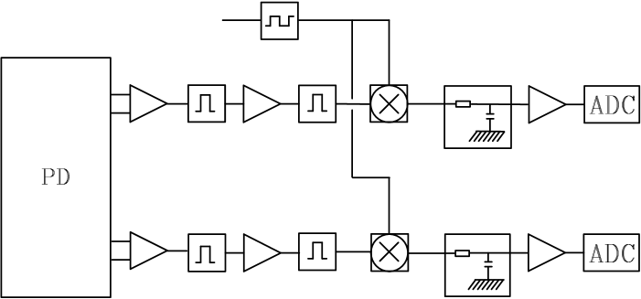
Figure 5: Post-detection segment of the polarimeter. The signal is filtered at the modulation frequency and amplified before the synchronous detection and the integration.

3 THE CALIBRATION PROCEDURE

3.1 The internal calibration mark

We use a calibration mark, as shown in Fig. 6, generated by a WR-28 Noise Source (NS) with an excess noise ratio $ENR\simeq 12\ dB$. The signal is divided by a waveguide power splitter (PS) and then injected into the amplification chains through a $20\ dB$ directional coupler (DC). Before entering the DC the signal is attenuated ($-30\ dB$) and guided into a stainless steel gold plated waveguides (WG). The two outputs of the diplexer are isolated using two ferrite circulators (Is). In this way we have a calibration correlated signal:

$$T_{cal}=T_{NS}\ exp[-(\tau_{PS}+\tau_{Att}+\tau_{Is}+\tau_{WG}+\tau_{DC})]$$ (13)

$T_{cal}\sim 20\ mK$

Unfortunately we also have a correlated signal when the NS is off. This is a possible source simulating a polarized sky signal. This spurious signal is at most the dummy load represented by the NS termination ($T_{0}^{NS}\sim 300\ K$), supposing to have a negligible return loss:

$$T_{spur}=T_{0}^{NS}\ exp[-(\tau_{PS}+\tau_{Att}+\tau_{Is}+\tau_{WG}+\tau_{DC})]$$ (14)

$T_{spur}\sim 1\ mK$

This is a correlated off-set signal which can be easily taken into account. What can be actually much more dangerous is the fluctuation of this level. These fluctuations can be set only by a thermal origin, in fact, when the NS is off, the source of spurious signal is a completely passive device. It is therefore extremely important to keep under control the temperature of the source of correlated signal. For this purpose we thermalize the NS and its case together with the diplexer at a temperature fluctuating not more than $\pm 0.1\ K$. In this way we have a fluctuation on the correlated signal: $\Delta T_{spur}<1\mu K$.

Figure 6: The internal calibration source. The signal from the noise source (NS) is divided by a power splitter (PS). In each chain we have an isolator (Is), a $30\ dB$ attenuator (Att), and a directional coupler (DC) used to inject the signal into the amplification chains.

The sky signal can be evaluated from this mark by taking into account the attenuation of the front-end of the radiometer (horn, fiberglass waveguide, window, Iris polarizer, ortho-mode transducer, and cryogenic isolators): $\tau_{FE}=\tau_{horn}+\tau_{win}+\tau_{FGW}+\tau_{OMT}+\tau_{Iris}+\tau_{CIs}$. The phase difference added by the NS path length ($\gamma^{\prime}$), respect to the phase of the signal entering the horn ($\gamma$), has to be also taken into account. Finally we get the following conversion factors ($\beta$) for the two outputs:

$$\beta_{1}(K/ADU)={T_{cal}\over O_{1,cal}}\ {\cos(\gamma^{\prime})\over\cos(\gamma)}\ e^{\tau_{FE}}$$ (15)

$$\beta_{2}(K/ADU)={T_{cal}\over O_{2,cal}}\ {\sin(\gamma^{\prime})\over\sin(\gamma)}\ e^{\tau_{FE}}$$ (16)

The phase difference of the NS correlated signal can be easily measured using the phase shifter placed in the amplification chain. We use this internal calibrator injecting it periodically in order to check for gain and phase long term fluctuations in the system. The NS is not able to measure the phase $\gamma$. This will be done using an external calibration source.

3.2 The external calibration source

The external source is a grid polarizer placed in front of the horn, at a distance far enough ($\sim 50\lambda$) to stay in the far-field region of the antenna. This grid has been realized with thin gold coated copper wires $0.3\ mm$ in diameter. The step of the wires is $s=0.6\ mm$, therefore we get a transmission coefficient of the perpendicular component of the radiation similar to the reflectivity of the parallel component. Both these coefficients are $\sim 99\%$. The dimensions of the grid are $50\ mm\times 50\ mm$.

The correlated signal produced by the grid is large, but its surface cover a small fraction ($\sigma\sim 19\%$) of the antenna beam. The signal is the sum of the antenna temperature ($T_{sky}+T_{Atm}$) transmitted by the grid and the noise temperature ($T_{N}^{Is}$) reflected back to the radiometer. In our case $T_{N}^{Is}\sim 20\ K$ is the temperature of the two cryogenic isolators placed at the output of the OMT. If the two isolators are at the same temperature, the correlated signal generated by the calibrator is[21]:

$$T_{grid}=\sigma[T_{sky}+T_{Atm}+T_{N}^{Is}]\times\cos(\theta)\sin(\theta)$$ (17)

Here $\theta$ is the angle between the grid’s wires and the principal planes of the OMT. If we rotate the grid we get the full characterization of this calibration signal. We have already tested this calibration system during the observations carried out from Dome Concordia on the Antarctic plateau during the local summer 1998-99[21, 22].

3.3 The power monitors

In addition to the described calibrators we can also measure the total power from the two amplification chains. These signals can be derived just before the Phase Discriminator by using two $20\ dB$ directional couplers (see Fig. 3). This information is useful to take under control the gain fluctuation of the RF and IF segments of the system.

Besides we can use these signals for calibration purpose and to evaluate the system noise temperature. The total power outputs can be calibrated using absorbers at two different temperature (liquid nitrogen and room temperature). In this way we get the sensitivity ($K/ADU$) and the noise temperature of the total power channels.

4 ANALYSIS OF SYSTEMATICS AND SENSITIVITY

An unavoidable requirement for an experiment devoted to the measurement of the CMB polarization is the stability of the performances. This is mandatory to guarantee the noise suppression during long integrations. In particular for correlation receivers the minimum detectable signal is related to the gain fluctuation ($\Delta G$) and to the offset ($T_{off}$) generated by the instrument:

$$\Delta T_{rms}=\sqrt{{\alpha\ T^{2}_{sys}\over\Delta\nu\ \tau}+T^{2}_{off}\Bigl{(}{\Delta G\over G}\Bigr{)}^{2}+\Delta T^{2}_{off}}$$ (18)

Here $\alpha$ is a numeric factor depending of the radiometer type, $\tau$ is the integration time, and $\Delta\nu$ is the bandwidth. The first term represent the white noise related to the system temperature of the radiometer. The other terms are degrading the system sensitivity, especially for long time integrations. In fact while the first term is decreasing with time the other contributions are expected to increase. Therefore gain stabilization and offset reduction are necessary to improve the sensitivity.

The offset signals arise mainly by non ideal performances of the system. In a correlation receiver spurious correlated signals are generated also in presence of uncorrelated radiation only. These signals can be produced only in the common parts, where the signals propagate in the same device. The places where this happens are the antenna (horn, iris polarizer, ortho-mode transducer) and the phase discriminator.

In a direct detection receiver into the second and third terms we have to put $T_{sys}$ ($\Delta T_{sys}$) in place of $T_{off}$ ($\Delta T_{off}$). The difference can be several order of magnitudes: $T_{sys}/T_{off}\sim 10^{4}-10^{5}$. This simple consideration suggests why a correlation receiver is intrinsically more stable than a direct detection one.

4.1 The antenna

Several spurious terms cane be generated on the antenna. The correlation introduced by the feed horn is responsible for an offset term related to the anisotropy of the sky radiation [23]. The signal is also proportional to the product of the co-polar and cross-polar radiation pattern of the antenna. A reasonable value of this product is $\sim 10^{-2}$, therefore this term is completely negligible, when the main contributor of the sky signal is the CMB.

A more serious effect comes from the cross correlation generated by the iris polarizer and by the ortho-mode transducer. The offset signal can be written as follows [23]:

$$T_{off}^{Iris+OMT}=SP_{OMT}(T_{sky}+T_{Atm}+T_{N}^{Ant})+SP_{Iris}\Bigl{(}T_{sky}+T_{Atm}+T_{N}^{Horn}-{T_{0}^{Iris}\over e^{-\tau^{*}_{horn}}}\Bigr{)}$$ (19)

$$T_{N}^{Ant}=T_{N}^{Horn}+{T_{N}^{Iris}\over e^{-\tau^{*}_{horn}}}+{T_{N}^{OMT}\over e^{-\tau^{*}_{horn}}\ |S_{L}|^{2}}$$ (20)

$$SP_{OMT}=2{\Re(S_{A1}S_{B1}^{*})\over|S_{A1}|^{2}}$$ (21)

$$SP_{Iris}={1\over 2}\Bigl{(}1-{|S_{C}|^{2}\over|S_{L}|^{2}}\Bigr{)}$$ (22)

There are two distinct terms. The first is related to the non ideality of the OMT. In fact it is proportional to the cross coupling term $S_{B1}$ (or $S_{A2}$). Here we suppose that the diagonal terms of the scattering matrix are $S_{A1}\sim S_{B2}\sim 1$, while the cross coupling terms are $S_{B1}\sim S_{A2}<<1$. The second term is generated by the Iris polarizer. Here we suppose $S_{L}\sim S_{C}$. This second term is not present when the polarimeter is operated without Iris polarizer. The contributions are also related to the noise temperature of the antenna components ($T_{N}^{Horn}$, $T_{N}^{Iris}$, $T_{N}^{OMT}$), to the external radiation field ($T_{sky}$, $T_{Atm}$), and to the physical temperature of the Iris polarizer ($T_{0}^{Iris}$).

In the previous formulae we have defined: $\tau^{*}_{horn}=\tau_{horn}+\tau_{win}+\tau_{FGW}$; while $T_{N}^{Horn}=T_{N}^{feed}+T_{N}^{win}+T_{N}^{FGW}$. For our polarimeter we have [18]: $T_{N}^{Horn}\sim 20-30\ K$, while $T_{N}^{Iris}+T_{N}^{OMT}\leq 1\ K$, and $T_{sky}+T_{Atm}\sim 10-15\ K$. The cross correlation term of the OMT is $S_{B1}\sim S_{A2}\sim-40\ dB$. We also estimate to have the same term from the Iris polarizer. Therefore the offset signal produced is: $T_{off}^{Iris+OMT}\sim few\ mK$. These components can change the physical temperature by about 1%, and anyway we monitor this variation and are able to correlate it with the observed offset signal.

One more term ($T_{off}^{RL}$) arises from the return loss of the antenna ($R_{Ant}$). The signal radiated from one of the ports of the OMT can be partially reflected and enter into the other port of the OMT. This signal is $T_{back}\sim T_{N}^{Is}+I_{Is}T_{HEMT}$. Here $I_{Is}\sim-20\ dB$ is the isolation of the cryogenic circulators. At the Phase Discriminator this signal is correlated with the radiation field propagating forward: $T_{for}\sim T_{Ant}+T_{HEMT}+I_{Is}T_{N}^{Is}$. At the PD output we obtain:

$$T_{off}^{RL}\sim(T_{HEMT}+T_{N}^{Is})\sqrt{I_{Is}\ R_{Ant}\ (SP_{OMT}+SP_{Iris})}$$ (23)

This term can be potentially of the same order of magnitude of $T_{off}^{Iris+OMT}$.

4.2 Modulation and correlation

Spurious signals can be also generated by the non ideal performances of the modulation/demodulation system and of the phase discriminator. We have seen as the combination of these devices erases the offset signal due to the lack of cancellation on the common mode terms[20]. The $AC$ detection technique helps also to improve the stability of the instrument performances, reducing the $1/f$ noise[20]. The frequency of the phase modulation is $\nu_{m}=781.25\ Hz$. This frequency has been chosen taking into account the major contributor of electromagnetic pollution, i.e. the electrical power supply network. Therefore we avoided to stay too close to the $50\ Hz$ harmonics (and the 60 $Hz$ too)[24].

The phase modulator is a pin-diode switch connecting input and output through two different path lengths. The two paths are selected reversing the polarization of the device. Both diodes and micro-strip lines present an attenuation. If the attenuation through the two ways is not the same an amplitude modulation is introduced together with the phase one. Even if the amplitude modulation is not so deep, the effect can be huge when an unpolarized source is observed.

If an amplitude asymmetry ($\delta<<1$) is present, on the $A$ channel, as it is the modulated one, the output signals, after the synchronous detection, are:

$$O_{1}=\Gamma[(h_{1}-h_{2})|A|^{2}\delta+(h_{1}+h_{2})\ 2AB\ (1+\delta/2)\ \cos(\gamma)]$$ (24)

$$O_{2}=\Gamma[(h_{3}-h_{4})|A|^{2}\delta+(h_{3}+h_{4})\ 2AB\ (1+\delta/2)\ \sin(\gamma)]$$ (25)

Two terms are now added to the one taking the information of the correlation. One of these terms is only a minor ($\delta<<1$) correction of the correlated signal. The other effect is to introduce a term depending on the common mode ($|A|^{2}$). This term can be reduced if the gains at the Phase Discriminator outputs are equalized, and the asymmetry in the amplitude modulation ($\delta$) minimized. The equalization of the outputs can be done by means of the resistive partitions placed before the differential amplifiers (see Fig. 4). The modulation asymmetry $\delta$ can be minimized by fine tuning the pine-diodes bias amplitude.

This spurious term enters into the output signal as an offset, but fluctuations in the system performances can mimic a correlation signal. We have analyzed also displacements from the ideal performances of the PD. Both amplitude asymmetries and phase couplings at angles different from the $90^{\circ}$ and $180^{\circ}$ induce only losses in the efficiency of the PD, but no spurious signal is generated.

5 OBSERVATION STRATEGY AND PROGRAMS

The instrument has been tested at the top of the Physics Department at the University of Milano - Bicocca for several months. These measurements have been devoted to debug the instrument from the systematics described previously testing the solutions adopted. In order to get high sensitivity the instrument performances have to be stable. This condition is required for long time integration. The instrument is operated inside a thermally insulating shelter. This solution has been adopted in order to create a stable environment around the radiometer. In this way we are able to thermalize the instrumentation and suppress the gain fluctuation. The horn is looking at the sky through a hole. We have selected an insulating tent operating down to a temperature of $-70^{\circ}C$. In fact one of observing sites selected for the polarimeter is the Antarctic plateau, during the local winter. Therefore this solution is ideal also in places with extreme climatic conditions. Besides the shelter is light and easily transportable[19].

The polarimeter will start celestial observations from Testa Grigia at the Plateau Rosà [25] on the Italian Alps, at 3480 m a.s.l. The instrument will be installed looking directly at the sky. Therefore we will observe with an angular resolution of $7^{\circ}$ and $14^{\circ}$. Observations will be carried out in transit mode, avoiding any movement of the instrumentation and of the beam direction. This can help for reducing the fluctuation of the signal coming from the local sources (ground and atmosphere). Then the polarimeter will be placed at the focal plane of the MITO telescope. In this way we get an angular resolution of $10-20\ arcmin$ [25, 26].

In a second time the polarimeter will be operated from the Antarctic Plateau in order to take advantage of the long Antarctic night. There observations in quasi static weather conditions are possible, avoiding solar radiation disturbances. Natural targets are the South Celestial Pole (SCP) regions. We can cover circles as large as few beam size around the pole. Besides, when observing the SCP, in case of linear polarization a typical signature is expected:

$$O_{1}\propto\sin(4\pi{t\over T}+\phi_{\circ})$$ (26)

$$O_{2}\propto\cos(4\pi{t\over T}+\phi_{\circ})$$ (27)

Here $t$ is the sidereal time, and $T$ a sidereal day, while $\phi_{\circ}$ is an arbitrary phase angle.

- [1] M. J. Rees, “Polarization and spectrum of the primeval radiation in an anisotropic universe,” The Astrophys. J. Lett. 153, pp. L1–L5, 1968.
- [2] P. de Bernardis and the BOOMERanG collaboration, “A flat universe from high-resolution maps of the cosmic microwave background radiation,” Nature 404, pp. 955–959, 2000.
- [3] S. Hanany and the Maxima collaboration, “Maxima-1: a measurement of the cosmic microwave background anisotropy on angular scales of 10′ - 5∘,” The Astrophys. J. Lett. 545, pp. L5–L9, 2000.
- [4] N. W. Halverson and the DASI collaboration, “Degree angular scale interferometer first results: a measurement of the cosmic microwave background angular power spectrum,” The Astrophys. J. 568, pp. 38–45, 2002.
- [5] W. Hu and M. White, “A cmb polarization primer,” New Astronomy 2, pp. 323–344, 1997.
- [6] A. Kosowsky, “Introduction to microwave background polarization,” New Astronomy Rev. 43, pp. 157–168, 1999.
- [7] R. Subrahmanian, M. J. Kesteven, R. D. Ekers, M. Sinclair, and J. Silk, “An australian telescope survey for cmb anisotropies,” MNRAS 315, pp. 808–822, 2000.
- [8] R. B. Partridge, J. Nowakowski, and H. M. Martin, “Linear polarized fluctuations in the cosmic microwave background,” Nature 331, pp. 146–147, 1988.
- [9] G. P. Nanos, “Polarization of the blackbody radiation at 3.2 centimeters,” The Astrophys. J. 232, pp. 341–347, 1979.
- [10] E. Torbet, M. J. Devlin, W. B. Dorwart, T. Herbig, A. D. Miller, M. R. Nolta, L. Page, J. Puchalla, and H. T. Tran, “A measaurement of the angular power spectrum of the microwave background made from the high chilean andes,” The Astrophys. J. Lett. 521, pp. L79–L82, 1999.
- [11] P. M. Lubin and G. F. Smoot, “Polarization of the cosmic background radiation,” The Astrophys. J. 245, pp. 1–17, 1981.
- [12] G. Sironi, F. Cavaliere, M. Gervasi, G. Giardino, C. Malfanti, S. Mussio, A. Passerini, F. Pennelli, and G. Bonelli, “A search for polarization of the cosmic microwave background at 33 ghz - preliminary observations of the south celestial pole region,” in Astrophysics from Antarctica, G. Novak and R. H. Landsberg, eds., pp. 116–120, ASP Conf. Ser. 141, 1998.
- [13] E. J. Wollack, N. C. Jarosik, C. B. Netterfield, L. A. Page, and D. Wilkinson, “A measurement of the anisotropy in the cosmic microwave background radiation at degree angular scales,” The Astrophys. J. Lett. 419, pp. L49–L52, 1993.
- [14] M. M. Headman, D. Barkats, J. O. Gundersen, S. T. Staggs, and B. Winstein, “A limit on the polarized anisotropy of the cosmic microwave background at subdegree angular scales,” The Astrophys. J. Lett. 548, pp. L111–L114, 2001.
- [15] N. Caderni, R. Fabbri, B. Melchiorri, F. Melchiorri, and V. Natale, “Polarization of the microwave background radiation. ii. an infrared survey of the sky,” Phys. Rev. D 17, pp. 1908–1918, 1978.
- [16] B. G. Keating, C. W. O’Dell, A. D. Oliveira-Costa, S. Klawikowski, N. Stebor, L. Piccirillo, M. Tegmark, and P. T. Timbie, “A limit on the large angular scale polarization of the cosmic microwave background,” The Astrophys. J. Lett. 560, pp. L1–L4, 2001.
- [17] P. M. Lubin, P. Melese, and G. F. Smoot, “Linear and circular polarization of the cosmic background radiation,” The Astrophys. J. Lett. 273, pp. L51–L54, 1983.
- [18] G. Sironi, G. Boella, G. Bonelli, L. Brunetti, F. Cavaliere, M. Gervasi, G. Giardino, and A. Passerini, “A 33 ghz polarimeter for observations of the cosmic microwave background,” New Astronomy 3, pp. 1–13, 1998.
- [19] G. Sironi, E. Battistelli, G. Boella, F. Cavaliere, M. Gervasi, A. Passerini, D. Spiga, and M. Zannoni, “Polarimetry of the cosmic microwave background from the antarctic plateau,” Publ. Astron. Soc. Aust. 19, pp. 313–317, 2002.
- [20] D. Spiga, E. Battistelli, G. Boella, M. Gervasi, M. Zannoni, and G. Sironi, “Cmb observations: improvements of the performance of correlation radiometers by signal modulation and synchronous detection,” New Astronomy 7, pp. 125–134, 2002.
- [21] M. Zannoni, Search for residual polarization of the cosmic microwave background. Phd thesys, Astronomy and Astrophysics - University of Milano, 1999.
- [22] M. Gervasi, E. Battistelli, G. Boella, F. Cavaliere, A. Passerini, M. Zannoni, and G. Sironi, “Cosmic microwave background polarization search: the milano 33 ghz polarimeter,” in What are the prospects for Cosmic Physics in Italy?, S. Aiello and A. Blanco, eds., pp. 165–169, SIF Conf. Proc. 68, 2000.
- [23] E. Carretti, R. Tascone, S. Cortiglioni, J. Monari, and M. Orsini, “Limits due to instrumental polarization in cmb experiments at microwave wavelengths,” New Astronomy 6, pp. 173–188, 2001.
- [24] M. Gervasi, E. Battistelli, G. Boella, F. Cavaliere, A. Passerini, G. Sironi, and M. Zannoni, “The milano polarization experiment devoted to the study of the cosmic microwave background,” in Astrophysical Polarized Backgrounds, S. Cecchini, S. Cortiglioni, R. Sault, and C. Sbarra, eds., pp. 164–168, AIP Conf. Proc. 609, 2002.
- [25] M. D. Petris, E. Aquilini, M. Canonico, L. D’Addio, P. de Bernardis, G. Mainella, A. Mandiello, L. Martinis, S. Masi, B. Melchiorri, M. Perciballi, and F. Scaramuzzi, “Mito: the 2.6 m millimetre telescope at testa grigia,” New Astronomy 1, pp. 121–132, 1996.
- [26] M. D. Petris, M. Gervasi, and F. Liberati, “New far infrared and millimetric telescopes for differential measurements with a large chopping angle in the sky,” Applied Optics 28, pp. 1785–1792, 1989.