Testing general relativity by micro-arcsecond global astrometry

The global astrometric observations of a GAIA-like satellite were modeled within the PPN formulation of Post-Newtonian gravitation. An extensive experimental campaign based on realistic end-to-end simulations was conducted to establish the sensitivity of global astrometry to the PPN parameter $\gamma$, which measures the amount of space curvature produced by unit rest mass. The results show that, with just a few thousands of relatively bright, photometrically stable, and astrometrically well behaved single stars, among the $\sim 10^{9}$ objects that will be observed by GAIA, $\gamma$ can be estimated after 1 year of continuous observations with an accuracy of $\sim 10^{-5}$ at the $3\sigma$ level. Extrapolation to the full 5-year mission of these results based on the scaling properties of the adjustment procedure utilized suggests that the accuracy of $\simeq 2\cdot 10^{-7}$, at the same $3\sigma$ level, can be reached with $\sim 10^{6}$ single stars, again chosen as the most astrometrically stable among the millions available in the magnitude range $V=12-13$. These accuracies compare quite favorably with recent findings of scalar-tensor cosmological models, which predict for $\gamma$ a present-time deviation, $\left|1-\gamma\right|$, from the General Relativity value between $10^{-5}$ and $10^{-7}$.

1 Introduction

Since General Relativity’s (GR) first appearance, many alternative gravity theories have been proposed. Experiments were then needed not only to test the validity of GR against Newton’s theory, but also every alternative theory of gravity against all the others (Will will93 (1993), will01 (2001)).

The Parametrized Post-Newtonian formalism (PPN) takes the slow-motion, post-Newtonian limit of all the metric theories and exploits their similarities to give them a unique, coherent framework by introducing a set of 10 PPN parameters. Each theory is then characterized by a particular value for each of the PPN parameters.

The validity of the post-Newtonian expansion is confined to those physical situations in which the energy density, regardless to its specific form, is small. Considering the various physical cases, this means that gravity fields ($U$), velocities ($v$), pressure to matter density ratios ($P/\rho$), and internal specific energy densities $\Pi$, are all small quantities so that (Ciufolini & Wheeler ciufwheel (1995); Will will93 (1993))

$$\epsilon^{2}\equiv\frac{v^{2}}{c^{2}}\sim\frac{U}{c^{2}}\sim\frac{P}{\rho c^{2}}\sim\Pi\ll 1,$$

where $\epsilon\ll 1$ is the “smallness parameter”. The slow-motion hypothesis also implies that, for any quantity $A$, its time derivative is much smaller than its space derivative, so that (Misner et al. misnetal (1973))

$$\frac{\left|\partial A/\partial t\right|}{\left|\partial A/\partial x\right|}\sim\epsilon;$$

this makes the PPN framework particularly convenient for Solar System experiments (where e.g. $U/c^{2}\lesssim 10^{-5}$). Each experiment allows one to measure the values of some PPN parameters, so that the theories that do not match those values are ruled out.

The most investigated among the PPN parameters are $\gamma$ and $\beta$, which measure respectively the amount of space-curvature produced by unit rest mass and the amount of non-linearity in the superposition law of gravity.

In GR the parameters $\gamma$ and $\beta$ are both equal to 1, while other theories aiming at the formulation of a unified theory predict small deviations from the GR value. The most promising of such theories consider the existence of a scalar field which, along with the usual metric tensor, participates in the generation of gravity. For this reason, such theories are usually called scalar-tensor theories. As a consequence, the value of $\gamma$ predicted by the scalar-tensor theories of gravity deviates from 1, and it is generally an adjustable value. Moreover, Damour and Nordtvedt (damnordt (1993)) showed that scalar-tensor cosmological models contain a sort of attractor mechanism toward GR. In practice the value of $\gamma$ changes with time and, whatever the value at the birth of the universe, it tends to 1 as $t\to\infty$. The present-time value of $|1-\gamma|$ (i.e. its deviation from GR) depends on the efficiency of the attractor mechanism, and Damour and Nordtvedt calculate a value between $10^{-5}$ and $10^{-7}$. More recently, Damour et al. (2002a , 2002b ) have given a new estimation of $|1-\gamma|$, within the framework compatible with string theory and modern cosmology, which basically confirms the previous results⁽⁾.

Although optical astrometry provided the first direct test of GR by measuring the amount of light bending due to the gravitational pull of the Sun (Dyson, Eddington, and Davidson 1920), observing conditions from the ground have severely limited the possibility of this technique to contribute to the search for a scalar component of gravity. Radio astrometry has been able to achieve significantly better results, however it is again the observing conditions (especially the effects of ionosphere and troposphere) which are ultimately limiting its accuracy in measuring gravitational light deflection from the ground. Presently, $\gamma$ is known to an accuracy of $\sim 10^{-3}-10^{-4}$ (Will will01 (2001)), therefore well above the level necessary to detect the scalar component predicted by Damour and Nordtvedt.

The success of the mission Hipparcos has proven that going into space is the way for increasing the accuracy of astrometric measurements to more interesting values. By utilizing the measurements of Hipparcos, (Froeschlé et al. froeschle (1997); see also Mignard  mignard (2001)) were able to derive $\gamma$ with an accuracy comparable to that of the best radio experiment (Lebach et al.  lebach (1995)). Therefore, expectations are that the micro-arcsec ($\mu$-arcsec) accuracy targeted by the space missions SIM, approved by NASA, and GAIA, approved by ESA, will be able to measure $\gamma$ with a precision of 10^-5–10^-6 (Danner and Unwin danunw (1999)) or better (ESA redbook (2000), de Felice et al. defelice3 (2000)), positioning optical astrometry at the fore front of experimental gravitation.

In this article we focus our attention on the GAIA project, a space astrometry mission that has recently been confirmed as a Cornerstone mission of the ESA program of scientific satellites. GAIA is expected to be launched not later than 2012, with a possible window of opportunity in 2010. For this reason ESA has devised a mission implementation plan that will be able to cope with a 2010 launch.

GAIA is a scanning astrometric satellite which builds on the successful concept of the Hipparcos mission, but with order-of-magnitude improvements in, e.g., the number of objects observed and measurement precision. It will be essential for the scientific advancement in many branches of astronomy, and especially in the fields of stellar astrophysics and galactic astronomy (Perryman et al. macp (2001)). Here we report on the first thorough attempt at determining the accuracy with which GAIA could measure the parameter $\gamma$. This is done through a realistic end-to-end simulation which considers the satellite most relevant modes of observation, the relativistic environment in which such observations take place, and the expected single-measurement errors.

2 The Parametrized Post-Newtonian (PPN) Model

Using the Eddington-Robertson form of the PPN formalism (where only the parameters $\gamma$ e $\beta$ are considered), we have developed a model based on the assumptions that the only source of gravity is a spherical and non-rotating Sun and the observer is moving on a circular orbit. This scenario is consistent with that discussed in our previous papers (de Felice et al. defetal1 (1998), defetal2 (2001); hereafter Paper I and Paper II, respectively),where a non-perturbative approach was developed as a first attempt at modeling the GAIA observations in a rigorous relativistic environment. Therefore, the results discussed in this paper can directly be compared with the findings reported in those earlier works.

Under the above hypotheses the PPN metric becomes (Misner et al., misnetal (1973))

$$\mathrm{d}s^{2} = -\left[1\!-\!2\frac{M}{r}\!+\!2\beta\left(\frac{M}{r}\right)^{2}\right]\mathrm{d}t^{2}+$$ (1)

$$\left[1\!+\!2\gamma\frac{M}{r}\right]\left[\mathrm{d}r^{2}\!+\!r^{2}\left(\mathrm{d}\theta^{2}\!+\!\sin^{2}\theta\,\mathrm{d}\phi^{2}\right)\right]$$

where $r$, $\theta$, and $\phi$ are spherical coordinates centered on the Sun, $t$ is coordinate time, and $M$ is the geometrized mass of the Sun.

As observable we consider the cosine of the angle $\psi_{12}$ between two stars; it can be expressed as

$$\cos\psi_{12}=\frac{h_{\alpha\beta}k_{1}^{\alpha}k_{2}^{\beta}}{\sqrt{h_{\iota\pi}k_{1}^{\iota}k_{1}^{\pi}}\sqrt{h_{\rho\sigma}k_{2}^{\rho}k_{2}^{\sigma}}},$$ (2)

where $k_{1}^{\alpha}$ and $k_{2}^{\alpha}$ are the four-velocities of the photons reaching the observer (i.e. the four-vectors tangent to the photons’ null-geodesics) and $h_{\alpha\beta}=g_{\alpha\beta}+u_{\alpha}u_{\beta}$ is a tensor which projects to the rest frame of the observer, i.e., the GAIA satellite. Here $g_{\alpha\beta}$ and $u_{\alpha}$ are the space-time metric and the observer’s four-velocity, respectively.

As expected, the expression we found for the four-velocities of the photons $k^{\alpha}$ depends on both $\gamma$ and $\beta$; then, they could be made part of the data reduction process as unknown parameters, in addition to those describing position and velocity of the stars. However, $\beta$ enters the $k^{\alpha}$ as a second order term compared to $\gamma$ (see also Eq.(1)); therefore, it was decided not to consider $\beta$ in the derivation of the observation equations (see below) but to set it to 1, namely to its value in GR.

Following the method developed in Paper I and II, and after a lengthy calculation, we then obtained the linearized observation equation as function of the astrometric parameters (i.e., angular coordinates, parallaxes, and proper motions), and of $\gamma$ in the form (Vecchiato vecchiato (2000))

$$-\sin\psi_{12}(t) \delta\psi_{12} =A_{1}\,\delta\theta_{1}(t_{0})+B_{1}\,\delta\phi_{1}(t_{0})+$$ (3)

$$C_{1}\,\delta p_{1}+D_{1}\,\delta\mu_{\theta_{1}}+E_{1}\,\delta\mu_{\phi_{1}}+$$

$$A_{2}\,\delta\theta_{2}(t_{0})+B_{2}\,\delta\phi_{2}(t_{0})+$$

$$C_{2}\,\delta p_{2}+D_{2}\,\delta\mu_{\theta_{2}}+E_{2}\,\delta\mu_{\phi_{2}}+$$

$$F\,\delta\gamma,$$

where the coefficients are derived from the differentiation of the right-hand side of Eq.(2) with respect to each of the unknowns.

As in Paper II, parallax and (angular) proper motions are defined as

$$p\equiv r_{\oplus}/r,\qquad\mu_{\theta}\equiv\frac{{\rm d}{\theta}}{{\rm d}{t}},\qquad\mu_{\phi}\equiv\frac{{\rm d}{\phi}}{{\rm d}{t}};$$

here $r_{\oplus}$ is the Earth’s mean orbital radius, $r$ is the coordinate radial distance of the star from the Sun and $t$ is the coordinate time.

3 The end-to-end simulation

The simulation follows the procedure used in the previous non-perturbative works (Paper I and II), the main change being the presence of the new unknown $\gamma$ that modifies the design matrix of the system of condition equations.

First, we generate the set of true quantities, which define initial location and temporal evolution of the stellar positions on the celestial sphere and the true value of $\gamma$. This was set to its GR value, i.e., $\gamma$ = 1. The corresponding catalog values are calculated, as usual, by adding suitable root-mean-square (rms) errors to the true values. Next, we find the stellar pairs which can be observed by a satellite that sweeps the sky following a Hipparcos-like scanning law. Once the stellar pairs are known the true angular distances (from the true coordinates) are calculated, and the satellite observations are generated by perturbing these true arcs with the observational error in Table 1. The catalog arcs (from the catalog coordinates) are also computed at this stage. Only arcs joining stars lying in different fields of view (FOVs) were counted without degeneration.

The result of these two steps is the generation of the measured quantity, $-\sin\psi(t)\delta\psi$, and of the coefficients in Eq. (3) for the construction of the linearized condition equations for all of the pairs observed during the mission lifetime we decided to simulate. Finally, the least-squares solution of the system is found by means of a conjugate-gradient method, suitable for large and sparse matrices like ours, and the errors are computed by direct comparison to the true values.

The least-squares solution returns the estimates of the adjustments to the catalog values of the unknowns in Eq. (3), i.e., $\tilde{\delta\theta}$, $\tilde{\delta\phi}$, $\tilde{\delta\mu_{\theta}}$, $\tilde{\delta\mu_{\phi}}$, $\tilde{\delta p}$, and $\tilde{\delta\gamma}$. For the adjustment to the $\gamma$ parameter, the corresponding rms error is indicated with the symbol $\sigma_{\delta\gamma}$. Notice that this error is the same as the error of $\gamma$, $\sigma_{\gamma}$, as $\tilde{\gamma}=\gamma_{cat}+\tilde{\delta\gamma}$, where $\gamma_{cat}$ is the simulated catalog value of the deflection parameter. The symbols $\sigma_{\delta\gamma}$ and $\sigma_{\gamma}$ are both used in the reminder of this article.

4 Experiments and results

Parameter	Numerical value	Comment
orbital radius	$1.496\cdot 10^{11}$ m	same as Earth’s orbital radius ($R_{\oplus}$)
precession angle	$43^{\circ}$	same as solar aspect angle
precession speed of the spin axis	6.4 rev/yr
satellite spin period	128 min
angle between the	$54^{\circ}$
viewing directions
field-of-view	$1^{\circ}\!\!.6$
of each telescope
mission starting time ($t_{0}$)	$-T/2$	minimum correlation between
		coords. and proper motions
radius of the simulated sphere	2 mas	uniform density sphere
		of 500 pc in radius
catalog error on	2 mas
coordinates and parallax
catalog error on $\gamma$	$\sigma_{\gamma}=2\cdot 10^{-3}$
single-measurement error ($\sigma_{obs}$)	10 $\mu$arcsec	as expected for pairs of
		V $\sim 12-13$  mag stars

Table 1: Most relevant parameters common to all of the simulations. $T$ is the mission duration. For the dynamical simulations, the stars are generated within a uniform density sphere of 500 pc centered on the Sun (i.e., $p\geq 2$ mas). Of course, the distribution of the resulting sample of simulated stars is representative only of a (relatively) small portion of the actual Galaxy. Nevertheless, as mentioned in Paper II, the adopted values are sufficiently realistic for the immediate scope of this work, which is to gauge the sensitivity of GAIA to the estimation of $\gamma$.

4.1 An upper limit on the accuracy of $\gamma$

Before going into the details of our experimental campaign it is useful to show, through a simple order-of-magnitude calculation, what kind of accuracy can be expected for $\gamma$ with GAIA-like observations. This calculation starts from the consideration that the satellite measurements for the estimation of $\gamma$ can be thought of as “Eddington-like” measurements of very high precision but with the stars at some tens of degrees from the solar limb. Each observation contributes to the determination of $\gamma$ with a precision of $\Delta_{\gamma}\sim 10^{-2}-10^{-3}$ ⁽⁾. If $N$ is the number of such observations, the final accuracy will be approximately $\sigma_{\gamma}\sim\Delta_{\gamma}\cdot N^{-1/2}$. For a period of, say, 1.5 years of continuous operations and 6500 of the stars in the magnitude range V=12-13 mag, GAIA would provide (see below) about 450000 observations, thus $\sigma_{\gamma}\sim 3\cdot 10^{-6}$. In the calculation above we have disregarded the facts that the geometry of the GAIA observations is different (the gravitational deflection is “seen” through its differential effect along the arcs joining the star pairs) and that $\gamma$ is not the only unknown to be estimated. Therefore, that value of $\sigma_{\gamma}$ is clearly representative of a best case scenario, and it is used only for comparison in the following discussion.

The simulation campaign was split in two parts. The first part was devoted to test the new code written for the PPN model and to make sure that the results were compatible with those in Paper I and II, and with the empirical prediction for $\gamma$ derived above. The second set of experiments was destined to establish the relation describing the GAIA sensitivity to $\gamma$ as function of the number of stars. Such a relation can then be used to make predictions on the accuracy of $\gamma$ for any given number of stars.

4.2 Validation of the PPN model

Table 1 lists the values of the input parameters which were common to all of the simulation runs. The main difference with our earlier work is in the single-observation error $\sigma_{\rm obs}$, which is set here to 10 $\mu$arcsec. This is the value expected for the error of one arc joining pairs of equal-magnitude stars, approximately 5 magnitudes brighter than those utilized in our previous experiments, i.e., V$\sim$12 mag. The 10-$\mu$arcsec error is compatible with current estimates of the GAIA error budget for stars brighter than $V=12-13$ (ESA, redbook (2000))⁽⁾.

As for the $\gamma$ parameter, the starting (catalog) value for the PPN parameter is generated from the true value by adding an error of $\sigma_{\gamma}=2\cdot 10^{-3}$, which is comparable with current best estimates.

The new code was tested on different sets of 50 simulations, and each Monte-Carlo set was run with the same values of the input parameters to have statistically significant results. The results of this series of experiments is summarized in Table 2.

The first row is representative of the runs with a “static sphere”, i.e., the ideal situation where all the stars have no intrinsic motions and are located at such a large (infinite) distance that the parallactic motion due to the observer is also null. In this case, the location on the celestial sphere of the simulated stars is completely specified by their angular coordinates ($\theta$ and $\phi$). Therefore, each linearized observation equation, Eq.3, has only five unknowns, the four corrections to the angular coordinates of each star pair, and the adjustment to the $\gamma$ parameter.

The second row presents the results of the simulations with a “dynamical sphere”, i.e., the case where the stars move with time. For simplicity, only the parallax motion was simulated; the stars were generated within a uniform density sphere of 500 pc centered on the Sun, i.e., with parallaxes $p\geq 2$ mas (200 times the measurement error), and, as for the static case, with no intrinsic (cosmic) motion. Notice that the mission duration was increased to 2 years. According to the findings in Paper II, this is the minimum observation period required for a reliable reconstruction of the dynamical parameters.

$$\begin{array}[]{c|c|c|c|c|c|c|c|c}T&n^{*}&n_{obs}&Q&\sigma_{obs}/\sqrt{Q}&\sigma_{\delta p}&\sigma_{\delta\theta}&\sigma_{\sin\theta\,\delta\phi}&\sigma_{\delta\gamma}\cdot 10^{5}\\ \hline\cr 1.5&6500&453071&34.85&1.69&--&1.76&1.88&0.94\\ 2.0&5000&356061&23.74&2.05&2.05&1.31&1.75&1.92\\ \end{array}$$

Table 2: Summary of the results of the different sets of simulations utilized to test the new code developed for the PPN model. $Q$ is the number-of-observations to the number-of-unknowns ratio.

As expected, the true errors of the astrometric parameters given in Table 2 compare quite well with what was obtained in Papers I and II after taking into account the differences in the values of $Q$ and the factor of 10 in measurement errors, consistent with the 5-mag difference of the stars considered in the new experiments. In particular, the results reported in the last row of Table 2 of Paper II, reproduce very closely what shown in our Table 2 for a mission duration of $T$=2 years.

4.3 What accuracy on $\gamma$?

Of much greater interest is the fact that the errors of $\gamma$ after the sphere reconstructions shown in Table 2 are considerably close to the best-case value of $\sim$ 3$\cdot$ 10^-6 derived at the onset of this section (see also Table 4 in de Felice et al 2000).

This encouraging result brought us to consider a new set of simulations with the intent to study the accuracy of $\gamma$ for larger samples of stars. Indeed, the all-sky survey nature of the GAIA observations ensures that all of the objects in the magnitude range of interest will be observed during the operational life of the satellite. This means that, although the actual number will considerably reduce because of the stringent requirements on the intrinsic astrometric stability of the sources, millions of potential targets will be available for the “$\gamma$ experiment”. Unfortunately, the computing power needed to perform a data reduction simulation of such a size is beyond our present resources, therefore we had to resort to an alternative schema to find the desired answer. We generated 11 simulations of a static sphere, each consisting, as before, of 50 runs with the same initial conditions and the mission duration set to 1 yr. The number of stars was increased from $n^{*}$=5000 to the maximum extent possible, i.e., $n^{*}$=15000. The results are listed in Table 3.

$n^{*}$	$<n_{\mathrm{obs}}>$	$\sigma_{\delta\gamma}$
5000	$1.78\cdot 10^{5}$	$1.99\cdot 10^{-5}$
6000	$2.56\cdot 10^{5}$	$1.91\cdot 10^{-5}$
7000	$3.49\cdot 10^{5}$	$1.23\cdot 10^{-5}$
8000	$4.56\cdot 10^{5}$	$1.33\cdot 10^{-5}$
9000	$5.79\cdot 10^{5}$	$1.34\cdot 10^{-5}$
10000	$7.14\cdot 10^{5}$	$9.79\cdot 10^{-6}$
11000	$8.63\cdot 10^{5}$	$9.19\cdot 10^{-6}$
12000	$1.03\cdot 10^{6}$	$1.07\cdot 10^{-5}$
13000	$1.20\cdot 10^{6}$	$8.16\cdot 10^{-6}$
14000	$1.40\cdot 10^{6}$	$7.87\cdot 10^{-6}$
15000	$1.60\cdot 10^{6}$	$6.19\cdot 10^{-6}$

Table 3: Computed errors on the estimation of the PPN parameter $\gamma$. The numbers refer to the results of the eleven $T=1$ yr Monte-Carlo simulations with increasing $n^{*}$ (number of stars). In the second column $<n_{\mathrm{obs}}>$ is the mean number of observations for the 50 simulations.

A single simulation, of the 50 comprising each Monte-Carlo set, yields one value of the difference $\delta\gamma=\gamma^{*}-\tilde{\gamma}$(true $\gamma$ minus estimated $\gamma$); each simulation is then a measure of $\gamma^{*}$ affected only by random errors, and the sample of 50 $\delta\gamma$’s has a Gaussian distribution. The standard deviation of this distribution, $\sigma_{\gamma}$, is the measure of the error on $\gamma$ of each Monte-Carlo group of simulations (Table 3). For example, if a difference of $3\cdot 10^{-5}$ from the GR value, $\gamma^{*}$=1, is measured for $\gamma$ with an error of $\sigma_{\gamma}\simeq 6\cdot 10^{-6}$, this would be interpreted as a 5-$\sigma$ detection of a deviation from General Relativity.

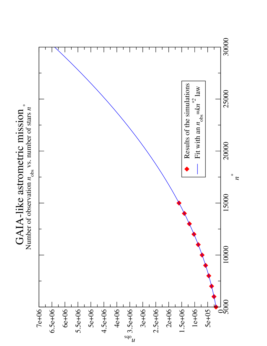
Figure 1: Number of observations versus number of stars. The solid curve represents the interpolated law $n_{\mathrm{obs}}$=$k\cdot{n^{*}}^{2}$, $k$=0.0071264.

Fig. 1 shows the relation $n_{\mathrm{obs}}$= $k\cdot{n^{*}}^{2}$ we derived from interpolating the data in Table 3. Also, simple statistical considerations suggest to fit the results in columns 2 and 3 of Table 3 to the $\sigma_{\delta\gamma}\propto n_{\mathrm{obs}}^{-1/2}$ relation, and the result is shown in Fig. 2.

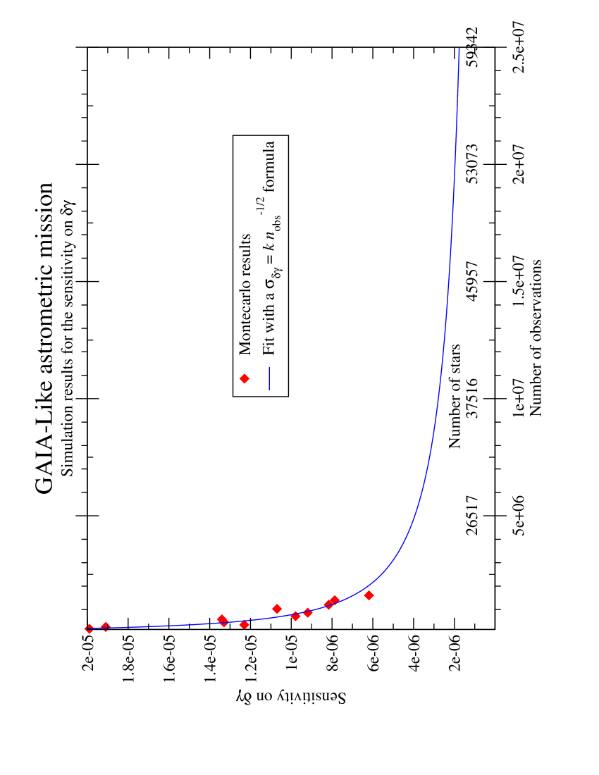
Figure 2: $\sigma_{\delta\gamma}$ versus number of observations. The solid curve represents the fit to the relation $\sigma_{\delta\gamma}=k\cdot n_{\mathrm{obs}}^{-1/2}$, $k=0.0088179\pm 0.0000097$.

We are now in a position to make realistic predictions on the error of $\gamma$ for a much larger number of stars (observations), comparable to the size of the stellar sample expected to be surveyed by the satellite at the magnitude limit of interest here. For $\sim 10^{6}$ stars ($\simeq$ $9.8\cdot 10^{8}$ observations), the value of $\sigma_{\delta\gamma}$ estimated from the curve in Fig. 2 is $\simeq 9\cdot 10^{-8}$. This means that a 1 yr-long GAIA-like mission could measure a value of $3\cdot 10^{-7}$ for $\left|1-\gamma\right|$, which would then represent a $3\sigma$ detection of the deviation of the actual gravitation from GR. And at the end of the satellite lifetime, after 5 years of continuous observations, the sensitivity to a $3\sigma$ detection will further improve by a factor of $1/\sqrt{2}$ to $\sim 2\cdot 10^{-7}$. These numbers imply that GAIA could reach the lower bound of the interval of possible deviations predicted by Damour and Nordtvedt (damnordt (1993)) and by Damour et al. (2002b ).

4.4 How do we compare with the Hipparcos result?

A Monte-Carlo experiment analogous to those above but with the relevant mission parameters set to the values of the Hipparcos mission was also conducted. We deemed it as quite important to compare our findings to the work of Froeschlé et al. (1997), who attempted the first direct determination of $\gamma$ by means of the global astrometric data taken with the Hipparcos satellite. Indeed, this would add confidence on the ability of our simulation to make realistic predictions on the possibility to derive a very accurate value for $\gamma$ with GAIA.

As “reference” experiment we adopted the case with 44000 stars in Table 1 of Froeschlé et al. (froeschle (1997)), which resulted in an error on the deflection parameter of $\sigma_{\gamma}=4\cdot 10^{-3}$.

We first simulated $n^{*}$=15000 stars and an observing period of 1 year; the observational and catalog errors were set to the values used in the Hipparcos experiments, i.e., $\sigma_{\mathrm{obs}}=3\,\mathrm{milli-arcsec}$ and $\sigma_{\mathrm{cat}}=1\,\mathrm{arcsec}$, respectively. The analysis of the usual 50 Monte-Carlo runs resulted in $\sigma_{\gamma}=2\cdot 10^{-3}$. We then scaled this value to the duration of the Hipparcos mission, 3 yr, and to the number of observations expected for 44000 stars (from the empirical law in Fig.1); this yielded $\sigma_{\gamma}=1\cdot 10^{-3}$.

That our experiment resulted in a much better value of $\sigma_{\gamma}$ should not come as a surprise, simply because we put ourselves in a more favorable situation: the instrument and satellite attitude were both assumed perfect in the simulation. In particular, having assumed a perfect astrometric instrument (optics, focal plane, and detectors) we disregarded any possible unmodeled systematic effect that could bias the estimation of $\gamma$, e.g., effects which would mimic a parallax zero-point error, as it has been the case for Hipparcos (Lindegren et al.  lennart (1992), Froeschlé et al. froeschle (1997)). In fact, in the observation equation derived from the reduction model used in the Hipparcos $\gamma$ experiment, one can see that the unknown which represents the parallax zero-point (common to all stars) is strongly correlated with the $\gamma$ parameter. It can be shown that, for the Hipparcos mission parameters, such correlation amounts to $\rho\simeq-0.92$ (Mignard mignard (2001)). A correlation of this magnitude, in turn, increases the error in the estimate of $\gamma$ by a factor of $1/\sqrt{1-\rho^{2}}\leavevmode\nobreak\ \simeq 2.6$ ⁽⁾. Therefore, the simulated “replica” of the Hipparcos experiment is to be considered consistent within a factor of 1.5, and not a factor of 4, with the published results based on the real data; quite an encouraging agreement given the quasi-ideal assumptions of our simulation.

5 Summary and conclusions

The global astrometric observations of a GAIA-like satellite were modeled within the PPN formulation of Post-Newtonian gravitation. Although simplified (a spherical and non-rotating Sun is the only source of gravity), this PPN model has allowed, through extensive end-to-end simulations, a realistic evaluation of GAIA’s sensitivity to the direct estimation of the light deflection parameter. The results show that the satellite could measure $\gamma$ to $\sim 10^{-7}$ ($1\sigma$) after 5 years of continuous observations, and using a subset of approximately $10^{6}$ stars chosen as the most astrometrically stable among the millions available in the magnitude range $V=12-13$ of the GAIA survey. Notice that after just one full year of observations $\gamma$ could be estimated with an error only a factor of $\sqrt{2}$ worse than the value above.

A comparison with the Hipparcos results has provided a way to gauge the degradation factor to be expected in going from an ideal instrument to the real astrometric payload and satellite. The factor of $1.5$ we found in that case is very encouraging; however, moving from the “milli-” to the “micro-”arcsec regime required by GAIA, the degradation might become larger. Future work will have to deal with the fact that the accuracy of $10^{-7}$ sets a goal for both the observational model, which will have to include all the details and the implications of Solar System gravitation, and instrument development and modeling, which will have to concentrate in identifying and, possibly, remove (through hardware improvements and/or calibration procedures), all relevant systematic error sources.

This work has provided quantitative evidence that the micro-arcsecond global astrometry of GAIA appears capable of testing general relativity to unprecedented levels. It will do so directly by accurately measuring the amount of light bending produced by gravity; a modern rendition, about a century later, of the experiment of Dyson, Eddington, and Davidson, then the first proof of Einstein’s theory.

6 Acknowledgements

We thank the referee for the valuable comments and for pointing us to the more recent literature.

Work partially supported by the Italian Space Agency (ASI) under contracts ASI I/R/32/00 and ASI I/R/117/01, and by the Italian Ministry for Research (MIUR) through the COFIN 2001 program.

References

- (1) Ciufolini, I., Wheeler, J. A., 1995; Gravitation and Inertia, Princeton Series in Physics
- (2) Danner, R. and Unwin, S. (eds.), 1999; SIM: Space Interferometry Mission. Taking the Measure of the Universe
- (3) Damour, T., Nordtvedt, K., 1993; Phys. Rev. Lett, 70, 2217
- (4) Damour, T., Piazza, F., Veneziano, G., 2002 (a); Phys. Rev. Lett, 89, 081601
- (5) Damour, T., Piazza, F., Veneziano, G., 2002 (b); Phys. Rev. D, 66, 046007
- (6) de Felice, F., Clarke, C.J.S., 1990; Relativity on curved manifolds, Cambridge University Press
- (7) de Felice, F., Lattanzi, M.G., Vecchiato, A., Bernacca, P.L., 1998; A&A, 332, 1133 (Paper I)
- (8) de Felice, F., Vecchiato, A., Bucciarelli, B., Lattanzi, M.G., Crosta, M.; 2000, IAU Colloquium 180, K. Johnston, D.D. McCarthy, B. J. Luzum, and G. H. Kaplan (Eds), p.314
- (9) de Felice, F., Bucciarelli, B., Lattanzi, M.G., Vecchiato, A., 2001; A&A, 373, 336 (Paper II)
- (10) Dyson, F.W., A.S. Eddington, & C. Davidson, 1920; Philosophical Transactions of the Royal Society of London 220A, 291
- (11) ESA 2000, GAIA: Composition, Formation and Evolution of the Galaxy, Technical Report ESA-SCI(2000)4, (scientific case on-line at http://astro.estec.esa.nl/GAIA)
- (12) Froeschlé, M., Mignard, F., and Arenou, F., 1997; Proc. of the ESA Symposium “Hipparcos - Venice ’97”, 13-16 May, Venice, Italy, ESA SP-402 (July 1997)
- (13) Lebach, D.E., Corey, B.E., Shapiro, I.I., et al., 1995; Phys. Rev. Lett., 75, 1439
- (14) Lindegren, L., van Leeuwen, F., Petersen, C., Perryman, M.A.C., and Söderhjelm, S., 1992; A&A, 258, 134
- (15) Mignard, F., 2001; GAIA: A European Space Project, O. Bienaymé and C. Turon (Eds), EAS Publication Series, Vol. 2, p. 107
- (16) Misner, C. W., Thorne, K. S., Wheeler J. A., 1973; Gravitation, Freeman
- (17) Perryman, M.A.C., de Boer, K.S., Gilmore, G., Høg, E., Lattanzi, M.G., Lindegren, L., Luri, X., Mignard, F., Pace, O., de Zeeuw, P.T., 2001; A&A, 369, 339
- (18) Vecchiato, A., 2000; General Relativistic Astrometry from Space. Theoretical Modeling and Software Implementation for Data Reduction, Ph.D. Thesis
- (19) Will, C. M., 1993; Theory and experiment in gravitational physics, Cambridge University Press
- (20) Will, C.M., 2001; Living Rev. Relativity 4, (2001), 4. [Online article]: cited on 19 Nov 2002 http://www.livingreviews.org/Articles/Volume4/2001-4will/