Analysis of the Flux and Polarization Spectra of the
Type Ia Supernova SN 2001el:
Exploring the Geometry of the High-velocity Ejecta
Abstract
SN 2001el is the first normal Type Ia supernova to show a strong, intrinsic polarization signal. In addition, during the epochs prior to maximum light, the CaII IR triplet absorption is seen distinctly and separately at both normal photospheric velocities and at very high velocities. The high-velocity triplet absorption is highly polarized, with a different polarization angle than the rest of the spectrum. The unique observation allows us to construct a relatively detailed picture of the layered geometrical structure of the supernova ejecta: in our interpretation, the ejecta layers near the photosphere ( km s-1) obey a near axial symmetry, while a detached, high-velocity structure ( km s-1) with high CaII line opacity deviates from the photospheric axisymmetry. By partially obscuring the underlying photosphere, the high-velocity structure causes a more incomplete cancellation of the polarization of the photospheric light, and so gives rise to the polarization peak and rotated polarization angle of the high-velocity IR triplet feature. In an effort to constrain the ejecta geometry, we develop a technique for calculating 3-D synthetic polarization spectra and use it to generate polarization profiles for several parameterized configurations. In particular, we examine the case where the inner ejecta layers are ellipsoidal and the outer, high-velocity structure is one of four possibilities: a spherical shell, an ellipsoidal shell, a clumped shell, or a toroid. The synthetic spectra rule out the spherical shell model, disfavor a toroid, and find a best fit with the clumped shell. We show further that different geometries can be more clearly discriminated if observations are obtained from several different lines of sight. Thus, assuming the high velocity structure observed for SN 2001el is a consistent feature of at least a known subset of type Ia supernovae, future observations and analyses such as these may allow one to put strong constraints on the ejecta geometry and hence on supernova progenitors and explosion mechanisms.
1 Introduction
1.1 Spectropolarimetry of Supernova
The geometrical structure of supernova ejecta, as determined empirically from observations, can give important clues as to the nature of the supernova progenitor system and explosion physics. Spectropolarimetry is a crucial tool in constraining the shape of unresolved supernovae. The scattering atmospheres found in supernovae can linearly polarize light. For an unresolved, spherically symmetric system the differently aligned polarization vectors around the disk will cancel, resulting in zero net polarization. If the symmetry around the line of sight is broken, however, a net polarization can result due to incomplete cancellation of polarization vectors (Shapiro & Sutherland, 1982).
The polarization observations of SN 2001el presented in Wang et al. (2002) (hereafter Paper I) are the first observations of a spectroscopically normal Type Ia supernova (SN Ia) which show a significant intrinsic polarization signal. Most previous observations of SN Ia showed no observable polarization, given the signal-to-noise of the observations (Wang et al., 1996). The only other indication of a clear non-zero polarization in a SN Ia was the subluminous and spectroscopically peculiar SN Ia 1999by, which showed an intrinsic continuum polarization of about 0.7 (Howell et al., 2001). Chemical inhomogeneities were also suggested to explain the rather noisy polarization data of SN 1996x (Wang et al., 1997). In addition, strong intrinsic polarization has been measured in all types of core collapse supernovae (Wang et al., 1996).
A non-zero intrinsic polarization measurement indicates that a supernova is aspherical, but using the spectropolarimetry to constrain the supernova geometry usually requires theoretical modeling. The detailed theoretical studies so far have been confined to axisymmetric configurations. Shapiro & Sutherland (1982) first estimated the continuum polarization expected from an ellipsoidal, electron scattering supernova atmosphere. Höflich (1991) used a Monte Carlo code to calculate the continuum polarization from several axisymmetric configurations, including an off-center energy source embedded in a spherical electron scattering envelope. Calculations of synthetic supernova polarization spectra have also been performed, but usually only for the ellipsoidal geometries (see however Chugai (1992)). In the past, such ellipsoidal models have done a fair job in fitting gross characteristics of the available spectropolametric observations, for example those of SNe 1987A (Jeffrey, 1991), 1993J (Höflich et al., 1996) and SN 1999by (Howell et al., 2001).
SN 2001el presents an exciting development in that no axially symmetric geometry is able to account entirely for the spectropolametric observations. In particular, we suggest that the supernova ejecta consists of nearly axially-symmetric inner layers ( km s-1), surrounded by a detached, high-velocity structure ( km s-1) with a different orientation. The analysis of the system therefore requires that we consider the synthesis of polarization spectra for 3-D configurations.
In this paper we take an empirical approach, and use a parameterized model to try to extract as much model independent information about the high velocity structure in SN 2001el as the observations will permit. A unique 3-D reconstruction of the geometry is not possible, as this constitutes a kind of ill-posed inverse problem. However, by restricting our attention to various parameterized systems, we can draw some rather general conclusions about the viability of different geometries. In particular, we examine the case where the inner ejecta layers are ellipsoidal and the outer, high-velocity structure is one of four possibilities: a spherical shell, an ellipsoidal shell, a clumped shell, or a toroid. We develop a technique for calculating 3-D synthetic polarization spectra of the high velocity material. The synthetic spectra rule out the spherical shell model, disfavor a toroid, and find a best fit with the clumped shell.
Geometrical information extracted empirically from spectropolarimetry must eventually be compared to detailed multi-dimensional explosion models. As of yet, none of the computed explosion models appear directly applicable to SN 2001el. 3-D deflagration models of a SN Ia in the early phases have been computed by Khokhlov (2000) and Reinecke et al. (2002). These models show a quite inhomogeneous chemical structure, with large plumes of burned material extending into unburned material. So far the calculations only cover the early stages of the explosion, before free expansion is reached. It is possible that at some point the deflagration transitions into a detonation wave (Khokhlov, 1991). The detonation may smooth out the inhomogeneities in the chemical composition by burning away the unburnt material between the plumes (Höflich et al., 2002; Khokhlov, 2000). It could also introduce a global asymmetry if it occurs at an off-center point (Livne, 1999). Other possible sources of asymmetry include rapid rotation of a white dwarf progenitor (Mahaffy & Hansen, 1975), and the binary nature of the progenitor system (Marietta et al., 2000).
1.2 Supernova SN 2001el
Monard (2001) discovered SN 2001el in the galaxy NGC 1448. The brightness of this nearby supernova ( at peak) made it an ideal candidate for spectropolarimetry. Spectropolametric observations were taken on Sept 25, Sept 30, Oct 9 and Nov 9 of 2001. Details on the observations and the data reduction of the spectra analyzed in this paper can be found in Paper I.
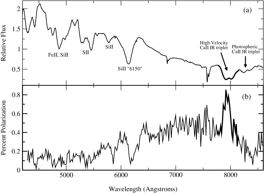
In Figure 1a we show the flux spectrum of SN 2001el for the first epoch (we have removed the redshift due to the peculiar velocity of the host galaxy). The flux spectrum of SN 2001el resembles the normal SN Ia SN 1994d at about 7 days before maximum light, with the expected P-Cygni features due to Si II, S II, Ca II and Fe II (see e.g. Branch et al. (1993)). The blueshifts of the minima of these features can be used to estimate the photospheric velocities of SN 2001el, which for all features are found to be km s-1. The only truly unusual feature of the flux spectrum is a strong absorption near 8000 Å, which is discussed in detail below.
We concentrate our analysis on the earliest spectrum (Sept. 25), of SN 2001el. A full description of the flux and polarization spectra at all epochs is given in Paper I.
1.3 High Velocity Material in SNe Ia
The most interesting feature of SN 2001el is the strong absorption feature near 8000 Å. The absorption has a “double-dipped” profile, consisting of two partially blended minima separated by about 150 Å. It seems to be a pure absorption feature with no obvious emission component to the red. The feature is still strong on Sept 30, but has weakened considerably by Oct 9. By the Nov 9 observations, the 8000 Å feature has virtually disappeared (see Paper I).
Hatano et al. (1999) identified a much weaker 8000 Å feature in SN 1994D as a highly blueshifted Ca II IR triplet. The double-dipped profile now visible in the Sept 25 SN 2001el spectrum supports this conclusion. The red-most line of the triplet (8662) produces the red-side minimum while the two other triplet lines (8542 & 8498) blend to produce the blue-side minimum. The synthetic spectra to be presented in §4 confirm that the IR triplet can reproduce the shape of the double minimum. Unfortunately, the early spectra do not extend far enough to the blue to observe a corresponding high velocity component to the Ca II H&K lines. We have investigated all other potential lines that might have caused the 8000 Å feature, but none were able to reproduce the feature without producing another unobserved line signature somewhere else in the spectrum.
Adopting the IR triplet identification for the 8000 Å feature, the implied calcium line of sight velocities span the range km s-1. This should be contrasted with the photospheric velocity of 10,000 km s-1 as measured from the normal SN Ia features in SN 2001el. We therefore make the distinction between the photospheric material, which gives rise to a seemingly normal SN Ia spectrum (hereafter, the “photospheric spectrum”), and the high velocity material (HVM), which produces the unusual 8000 Å IR triplet feature. In the flux spectrum, there is a clear separation between the photospheric triplet absorption at 8300 Å and the HVM feature at 8000 Å. In the polarization spectrum, the angle and degree of polarization of the 8000 Å feature each differ from the photospheric spectrum. Both of these imply a rather sudden change of the atmospheric conditions in the HVM.
A high velocity CaII IR triplet feature has been observed in other SNe Ia, albeit rarely and never as strong. The pre-max spectra of SN 1994D (Patat et al., 1996; Meikle et al., 1996), show a similar, but much weaker absorption. The Si II and Fe II lines of these spectra also suggest some material is moving faster than 25,000 km s-1 (Hatano et al., 1999) The earliest spectrum of SN 1990N at day -14 (Leibundgut et al., 1991) has a deep, rounded 8000 Å feature, and the spectrum also showed evidence of high velocity silicon or carbon (Fisher et al., 1997). The 8000 Å feature has also been observed in the maximum light spectrum of SN 2000cx (Li et al., 2001). In this case, however, the line widths are narrower and the two minima are almost completely resolved.
In SN 2001el, the only clear-cut evidence for high velocity material seems to be the 8000 Å feature. There is no strong Si II 6150 absorption at , although a weak absorption cannot be ruled out because at this wavelength (5880 Å) it would blend completely with the neighboring Si II feature. There is also no clear indication of high velocity Fe II or S II. The blue edge of the Ca II H&K feature on Oct. 9 – the first available spectrum to go far enough to the blue – is at 27,000 km s-1. The likelihood of this being HVM is suspect because of the strong possibility of line blending. Since the 8000 Å feature is the only unambiguous detection of a high velocity material in SN 2001el, we hereafter refer to it as the HVM feature.
Our analysis will focus almost entirely on the 8000 Å HVM feature. In §2 we give an introduction to polarization in supernova atmospheres; §3 describes a parameterized model that allows us to generate synthetic polarization spectra, and in §4 we use the model to explore various geometries for SN 2001el. In §5 we consider the signature of each geometry when viewed from alternative lines of sight. The implication of these constraints on the progenitors and explosion mechanisms of SNe Ia’s is discussed briefly in the conclusion.
2 Supernova Spectropolarimetry
2.1 Polarization Basics
The polarization state of light describes an anisotropy in the time-averaged vibration of the electric field vector. A beam of radiation where the electric field vector vibrates in one specific plane is completely (or fully) linearly polarized. A beam of radiation where the electric field vector vibrates with no preferred direction is unpolarized. Imagine holding a polarization filter in front of a completely linearly polarized light beam of intensity . The filter only transmits the component of electric field parallel to the filter axis. Thus as the filter is rotated, the transmitted intensity, which is proportional to the square of the electric field, varies as .
The light measured from astrophysical objects is the superposition of many individual waves of varying polarization. Imagine a light beam consisting of the super-position of two completely linearly polarized beams of intensity , and , whose electric field vectors are oriented 90∘ to each other. If the beams add incoherently, the transmitted intensity is the sum of each separate beam intensity:
| (1) |
If the beams are of equal intensity, , then the transmitted intensity shows no directional dependence upon – i.e. the light is unpolarized. In this sense, we say that the polarization of a light beam is “canceled” by an equal intensity beam of orthogonal – or “opposite” – polarization. If the cancellation is incomplete, and the beam is said to be partially polarized. The degree of polarization is defined as the maximum percentage change of the intensity; in this case:
| (2) |
The polarization position angle (labeled ) is defined as the angle at which the transmitted intensity is maximum.
It is tempting to think of the polarization as a (two dimensional) vector, since it has both a magnitude and a direction. Actually the polarization is a percent difference in intensity, and intensity is the square of a vector (the electric field). The polarization is actually a quasi-vector, i.e. polarization directions 180∘ (not 360∘) apart are considered identical. The additive properties of the polarization thus differ slightly from the vector case, as evidenced by the fact that the polarization is canceled by another equal beam oriented to it, rather than one at as in vector addition.
In this case, a useful convention for describing polarization is through the Stokes Parameters, and , which measure the difference of intensities oriented 90∘ to each other. A Stokes “Vector” can be defined and illustrated pictorially as:
| (3) |
where , for instance, designates the intensity measured with the polarizing filter oriented 90∘ to a specified direction called the polarization reference direction. To determine the superposition of two polarized beams, one simply adds their Stokes vectors. A fourth Stokes parameter measures the excess of circular polarization in the beam. Non-zero circular polarization has not been measured in supernova, and no circular polarization observations were taken for SN 2001el; therefore we will not discuss Stokes in this paper. For scattering atmospheres without magnetic fields, the radiative transfer equation for circular polarization separates from the linear polarization equations, allowing us to ignore in our calculations (Chandrasekhar, 1960).
We further define the fractional polarizations: and . The degree of polarization, , and the position angle can then be written in terms of the Stokes Parameters:
| (4) |
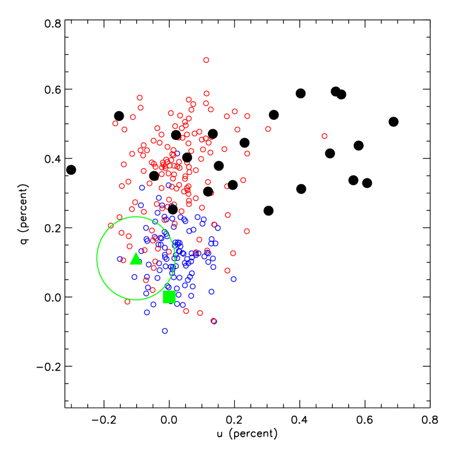
A single plot that captures both the change of polarization degree and position angle over a spectrum is the q-u plot of Figure 2. Each point in this figure is a wavelength element of the spectrum, and for each point we can read off and at that wavelength much as we would read a polar plot. According to Equation 4, the degree of polarization is given by the distance of the point from the origin, while the position angle is half that of the plot’s polar angle. In this sense and can be thought of as the two components of a two dimensional polarization quasi-vector.
2.2 Polarization in Supernova Atmospheres
The major opacities in a supernova atmosphere are due to electron scattering and bound-bound line transitions. The continuum polarization of supernova spectra is attributed to electron scattering. The line opacity can create features (either peaks or troughs) in the polarization spectra.
To understand the polarizing effect of an electron scattering, note that an electron scatters a fully polarized beam of radiation according to dipole angular distribution, where is the angle measured from the incident polarization direction. Now unpolarized light can be represented by a super-position of two equal intensity, fully-polarized orthogonal beams. Upon electron scattering, the two differently oriented beams get redistributed according to differently oriented dipole patterns; thus in certain directions they are no longer equal and do not cancel. The scattered light is therefore polarized with the percent polarization depending upon the scattering angle between incident and scattered rays:
| (5) |
Light scattered at 90∘ is fully polarized, while that which is forward scattered at 180∘ remains unpolarized. The direction of the polarization is perpendicular to the scattering plane defined by the incoming and outgoing photon directions.
Deep enough within the supernova atmosphere, the light becomes unpolarized for two reasons: (1) Below a certain radius, known as the thermalization depth, the absorptive opacity dominates the scattering opacity and photons are destroyed into the thermal pool. The energy is subsequently re-emitted as blackbody radiation which, being the result of random collision processes, is necessarily unpolarized. (2) Deep within the atmosphere, the radiation field becomes isotropic. Because the radiation incident on a scatterer is then equal in all directions, the net polarization of scattered light will cancel.
The polarization of the radiation occurs above the inner unpolarized depth, where the election scattering opacity dominates and the radiation field becomes anisotropic due to the escape of photons out of the supernova surface. We call this region the electron-scattering zone. The surface above the electron scattering zone at which point photons have a high probability of escaping the atmosphere, is the supernova photosphere. Formation of the well-know P-Cygni line profiles in supernovae is due to line opacity from material primarily above the photosphere. This region is called the line-forming region.
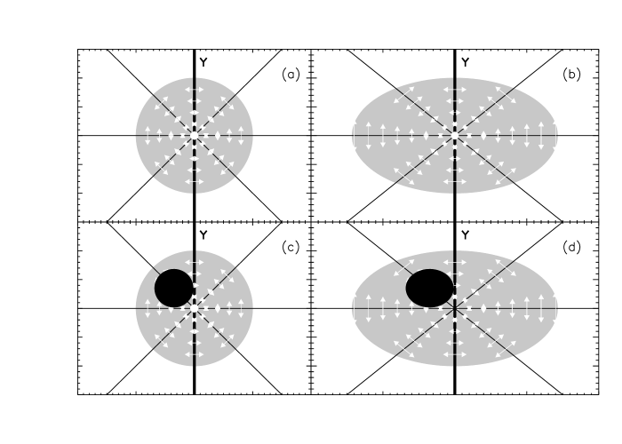
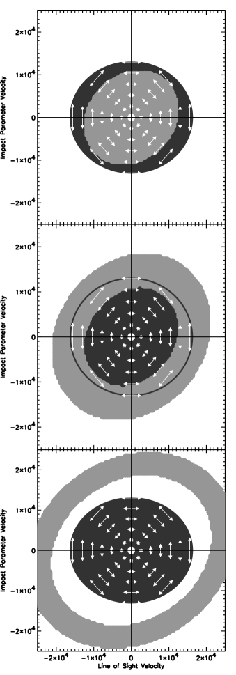
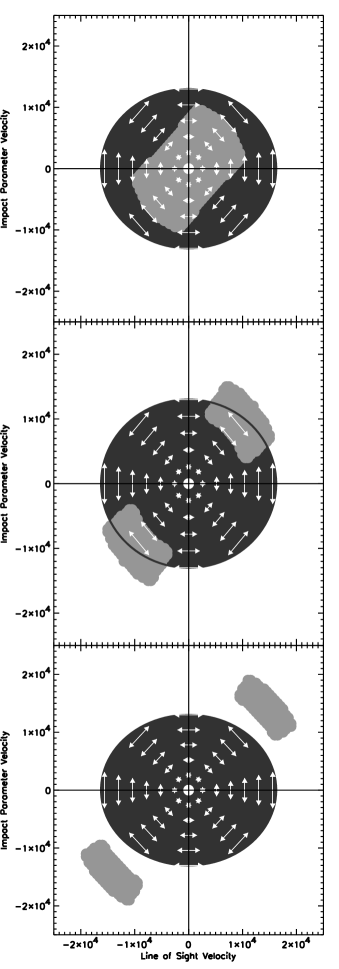
Figure 3 illustrates how the polarization of specific intensity beams emergent from an spherical, pure electron scattering photosphere might look. The double-arrows indicate the polarization direction of a beam, with the size of the arrow indicating the degree of polarization (not the intensity). Note the following two facts: (1) The polarization is oriented perpendicular to the radial direction. This follows from nature of the anisotropy of the radiation field. At all points in the atmosphere (except the center) more radiation is traveling in the radial direction than perpendicular to it. Because the polarization from electron scattering is perpendicular to the scattering plane, the dominant scattering of radially traveling light will produce an excess of polarization perpendicular to the radial direction. (2) The light from the photosphere limb is more highly polarized than that from the center. This is because the radiation field at the limb is highly anisotropic – i.e highly peaked in the outward (radial) direction. In addition, photons scattered into the line of sight from the supernova limb, have generally scattered at angles closer to 90∘.
If the projection of the supernova along the line of sight is circularly symmetric, as in Figure 3a, the polarization of each emergent specific intensity beam will be exactly canceled by an orthogonal beam one quadrant away. The integrated light from the supernova will therefore be unpolarized. A non-zero polarization measurement demands some degree of asphericity; for example in the ellipsoidal photosphere of Figure 3b, vertically polarized light from the long edge of the photosphere dominates the horizontally polarized light from the short edge. The integrated specific intensity of Figure 3b is then partially polarized with . Because an axisymmetric system has only one preferred direction, symmetry demands that the polarization angle is aligned either parallel or perpendicular to the axis of symmetry, thus for the geometry of Figure 3b.
The effect of line opacity on the polarization spectrum can be complicated. In general, light resonantly scattered in a line can become polarized in much the same way as described above for electrons. However because randomizing collisions tend to destroy the polarization state of an atom during an atomic transition, the light scattered from lines in supernova atmospheres is often assumed to be completely unpolarized (e.g. Höflich et al. (1996) – we discuss this assumption in more detail in §3.4). In ellipsoidal models, it has been shown that the effect of depolarizing line opacity is primarily to create a decrease in the level of polarization in the spectrum (Höflich et al., 1996). Because SN Ia have more lines in the blue, the polarization in such models typically rises from blue to red.
In general, however, the fact that a line is depolarizing does not mean it necessarily produces a decrease in the degree of polarization in the spectrum. The actual effect will depend sensitively upon the geometry of the line opacity and the electron scattering medium. For example, suppose the electron-scattering regime is spherical, but in an outer, detached layer there is an asymmetric clump of line optical depth, as shown in Figure 3c. Because the line obscures light of a particular polarization, the cancellation of the polarization of the photospheric specific intensity beams will not be complete. The line thus produces a peak in the polarization spectrum and a corresponding absorption in the flux spectrum. We call this effect of generating polarization features the partial obscuration line opacity effect or just partial obscuration. In the case of Figure 3c, the clump primarily absorbs diagonally polarized light, so we expect the polarization peak to have a dominant component in the u-direction.
A non-axially symmetric supernova is shown in Figure 3d. The electron scattering medium is ellipsoidal, so the continuum spectrum will be polarized in the q direction. The clump of line opacity, which breaks the axial symmetry, preferentially obscures diagonally polarized light so the line absorption feature will be polarized primarily in the u direction. As we see in the next section, this type of two-axis configuration is a relevant one for SN 2001el.
2.3 The Polarization of SN 2001el
2.3.1 Polarization of The Photospheric Spectrum
The q-u plot of SN 2001el is shown in Figure 2. In order to interpret the intrinsic supernova polarization, one must first subtract off the interstellar polarization (ISP), caused by the scattering of the radiation off aspherical dust grain along the way to the observer. The ISP has a very weak wavelength dependence, (Serkowski et al., 1975) and therefore choosing the magnitude and direction of the ISP is basically equivalent to choosing the zero point of the intrinsic supernova polarization in the q-u plane of Figure 2. The particular choice of ISP can dramatically affect the theoretical interpretation of the polarization data (see Leonard et al. (2000); Howell et al. (2001)).
The choice of the ISP that leads to the simplest theoretical description is shown as the green square in Figure 2. In this case the photospheric part of the spectrum (open circles), apart from some scatter, draws out a straight line in the q-u plane – i.e. the degree of polarization changes across the photospheric spectrum but the polarization angle remains fairly constant. This would be the case if all of the photospheric material followed the same axial symmetry. The intrinsic polarization spectrum (i.e. percent polarization versus wavelength) of SN 2001el using this choice of ISP is shown in Figure 1b. The degree of polarization rises from blue to red, as expected in ellipsoidal models due to the higher line opacity in the blue. The level of continuum polarization in the red is about 0.4%, and the SiII 6150 line represents a depolarization by about the same amount. Models of ellipsoidal electron scattering atmospheres indicate that level of polarization may roughly correspond to an deviation from spherical symmetry of about (Höflich, 1991).
Although the square in Figure 2 is favored by simplicity arguments, it is preferable to make a direct measurement of the ISP, if possible. At late epochs it is believed that the supernova ejecta becomes optically thin to electron scattering. The intrinsic supernova continuum polarization would then be zero, and the observed polarization due only to the ISP. Paper I estimated the ISP in this way, using observations taken on Nov 9. Assuming the intrinsic supernova polarization is zero at this time, the determined ISP (with an estimated error contour) is shown as the green triangle in Figure 2 . Although the ISP thus determined is not grossly inconsistent with the simplest choice, it seems to indicate that the polarization zero point lies off of the main q-u line. If this is true, the angle across the photospheric spectrum is no longer constant. The photospheric material approximates an axial symmetry, but an off-axis, sub-dominant component (e.g. a photospheric clump) must exist to account for the offset of the q-u line.
Because the main purpose of this paper is to explore the geometry of the HVM, not the photosphere, we will simplify our discussion by ignoring any off-axis photospheric components. We will assume the polarization zero point of the axially-symmetric component is given by the square and that the photosphere can be approximately modeled as an ellipsoid. Although the paricular ISP choice has important implications for the geometry of the photospheric material, it does not greatly affect our analysis of the HVM feature.
2.3.2 Polarization of The HVM Feature
The HVM flux absorption feature is associated with a polarization peak in the spectrum (Figure 1b). Unlike the flux absorption profile, the polarization peak does not show a clear double feature. Although the noise of the polarization spectrum makes it difficult to analyze the line profile, it appears that a peak due to the red triplet line () is absent or suppressed compared to the blue lines ( & ).
In Figure 2, the wavelengths corresponding to the HVM feature are shown with closed circles. The HVM polarization angle deviates from the photospheric one, pointing instead mostly in the u-direction. The HVM feature also shows an interesting looping structure – as the wavelength is increased, the polarization moves counter-clockwise in the q-u plane. “q-u loops” such as these have been observed before, for example in the H-alpha feature of SN 1987A (Cropper et al., 1988).
The different polarization angle of the HVM feature means that the geometry of SN 2001el cannot be completely axially symmetric. The Stokes parameter changes sign upon reflecting the system about the polarization reference axis (see Equation 3) and therefore must be zero for any system with a reflective symmetry, such as the axially-symmetric system of Figure 3b. The non-zero u-polarization can not solely be a kinematic effect either, for although the SN ejecta is expanding, the velocity law is supposed to be a spherical, homologous one () which preserves the reflective symmetry. As the supernova expands and evolves the density contours of the system may change as outer layers thin out and reveal different parts of the underlying material; however unless the velocity law deviates from homology and shows some preferential direction, the reflective symmetry will always be preserved and we must have at all times. In order to get a non-zero u component, we must break the reflective symmetry of the geometry with an off-axis component, such as the clump of Figure 3d.
A natural explanation of the relatively large degree of polarization and change of polarization angle of the HVM feature is partial obscuration of polarized photospheric light, somewhat like Figure 3d. We find in §4 that this interpretation can also account for the q-u loop. In the next section we describe a technique for calculating partial obscuration that allows us to directly compare synthetic polarization spectra to the data. Other mechanisms could presumably be invoked to explain the HVM polarization peak, but in this paper we only consider the effects of partial obscuration.
3 The Two-Component Polarization Model
To compute polarization in multi-dimensions most investigators have employed Monte Carlo methods (Code & Whitney, 1995; Wood et al., 1996; Höflich, 1991). This approach has the benefits of generality and ease of coding, but with the drawback of extreme computational expense. A very large number of photons must be followed to escape along each line of sight in order to overcome the random Poisson noise. This noise must be kept much less than a fraction of a percent in order to confront the small observed polarization levels. It is therefore cumbersome to use Monte Carlo codes in a parameterized way to explore the huge parameter space available with 3-D geometries.
In the case of the HVM, a simplification is possible that allows for a much faster and more insightful computation. Assuming that the electron densities in the HVM regime are around , the optical depth to electron scattering through the HVM shell is . Therefore one can ignore electron scattering in the HVM and the radiative transfer problem separates naturally into the two regimes of photosphere and HVM. The photosphere acts as a source of polarized light illuminating a region of basically pure line optical depth in the HVM. Assuming the lines are depolarizing, the only effect of the HVM is to obscure some of the polarized photospheric light and re-emit some unpolarized light into the observer’s line of sight.
Because the model makes a sharp distinction between an inner polarized source (the photosphere) and an outer line-forming region (the HVM), we call this approach the two-component model. The model is basically a way to formalize the simple pictures of Figure 3. The two-component model is constructed to apply to the detached layers of the HVM. For line forming material near the photosphere a sharp separation of the two regimes would be artificial since electron scattering is not entirely negligible in the line forming region. Because the two-component model does not account for the multiple scattering between lines and electrons, photospheric spectra synthesized with it may be incorrect. On the other hand because the model captures some of the essential features of various geometries, some qualitative insight may still be gained with respect to the lines formed near the photosphere. As we are only concerned with the HVM in this paper, this is not relevant for the present work.
3.1 The Sobolev Approximation
The Sobolev approximation is a method for computing line formation in atmospheres with large velocity gradients. Sobolev models (under the assumption of a sharp photosphere plus line forming region) have frequently been used to analyze supernova flux spectra. Typically spherical symmetry is assumed (e.g. (Branch et al., 1983; Hatano et al., 1999)) but the method has also been applied in 3D (Thomas et al., 2002). Derivations of the Sobolev method and justification of the approximation in the modeling of supernova atmospheres can be found in (Rybicki & Hummer, 1978; Castor, 1970; Jeffery & Branch, 1990); here we only quote the important results.
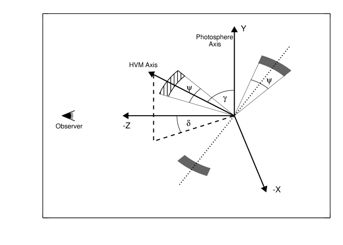
The geometry used in the models is shown in Figure 4. We use a cylindrical coordinate system, or alternatively a Cartesian one . In either case the observer line of sight is chosen as the axis with decreasing toward the observer (i.e. the observer is at negative infinity). The polarization reference axis is chosen to lie along the (or y) direction, which is also the photosphere symmetry axis.
For atmospheres in general expansion, such as supernovae, the wavelength of a propagating photon is constantly redshifting with respect to the local comoving frame of reference. The insight behind the Sobolev approximation is that the photon will only interact with a line in the small region of the atmosphere where the photon is Doppler-shifted in resonance with the line. The radiative transfer problem then becomes localized to such “resonance regions”. Free expansion is established in supernova atmospheres shortly after the explosion; the velocity vector at a point in the atmosphere is in the radial direction and is given by , where is the radius at time since explosion, and is the initial radius which is usually small and can be ignored. Consider a beam of radiation emanating from the photosphere and propagating through this atmosphere in the direction, at an impact parameter and azimuthal angle . Such a beam was illustrated pictorially as a double-arrow in Figure 3; here we quantify it with a Stokes specific intensity vector . If the wavelength of the beam in the observer frame is , then the wavelength in the local comoving atmosphere frame is given by the (non-relativistic) Doppler formula:
| (6) |
Suppose the only opacity in the atmosphere is due to one line with rest wavelength . A beam of radiation will come into resonance with the line when , which by Equation 6 is at a point:
| (7) |
For each wavelength in an observed spectrum there is thus a unique point in the z-direction at which the beam comes in resonance with the line. According to the Sobolev approximation, the emergent Stokes specific intensity that reaches the observer at infinity after passing through the line forming region is given by:
| (8) |
where is the Sobolev line optical depth at the point and is the Stokes source-function of the line at this point. Both quantities will be explained further in the sections to come. The first term in Equation 8 represents photospheric light attenuated by the line optical depth; the second term represents light scattered or created to emerge into the line of sight by the line. Equation 8 is identical to the usual, unpolarized expression for the Sobolev approximation (see Rybicki & Hummer (1978)), except now the terms in boldface are all Stokes vectors.
To generate the observed spectrum of an unresolved object, the specific intensity of Equation 8 must be integrated over the projected surface of the atmosphere, i.e. over the plane. A wavelength in the observed spectrum thus gives us information about the line optical depth and source function integrated over a plane at . Such a plane, which is perpendicular to the observer’s line of sight, is called a constant-velocity (CV) surface.
In the case of an monotonically expanding atmosphere with more than one line, a beam of radiation will come into resonance with each line one at a time, starting with the bluest line and moving to the red. In this case Equation 8 is readily generalized:
| (9) |
where the indices i and j run over the lines from red to blue. Before considering the integration of Equation 9 over the CV planes, we discuss in more detail the terms , , and .
3.2 The Photospheric Intensity
In this section we calculate the intensity and polarization of specific intensity beams emergent from an electron scattering photosphere. We first consider in the case that photospheric regime is spherical (as in Figure 3a) and later show how to adapt the result to the ellipsoidal case. From the circular symmetry, the intensity and degree of polarization of a specific intensity beam can only depend upon the impact parameter and not on . Let represent the specific intensity in the direction at , and the degree of polarization of this beam. The polarized specific intensity is which will be divided between the and Stokes parameters.
For , the polarization points in the horizontal, or negative direction – i.e. while . The Q and U components at arbitrary are derived by rotating this expression by . The resulting Stokes vector is:
| (10) |
The fact that the trigonometric rotation terms depend on rather than reflects the fact that the polarization is actually a quasi-vector (Chandrasekhar, 1960).
In the two-component model one must pre-compute the functions and . Chandrasekhar first obtained the result for a pure electron scattering, plane-parallel atmosphere (Chandrasekhar, 1960); in that case follows closely the linear limb darkening law, while the degree of polarization rises from zero in the center to at the limb; however, the plane-parallel approximation is not a good one for supernovae, which have extended atmospheres (i.e. the thickness of the electron scattering zone is a sizable percentage of its radius). In an extended atmosphere the radiation field tends toward a more anisotropic distribution, peaking in the outward direction. This increased anisotropy of the radiation field leads to generally higher limb polarizations. Cassinelli & Hummer (1971) solved the polarized radiative transfer Equation for extended, spherical electron scattering spheres with density power laws of index n=2.5 and n=3. They find the polarization can become higher than at the limb.
We model the photospheric regime as an inner unpolarized boundary surface, surrounded by a pure electron scattering envelope with a power law electron density . We choose , a density law motivated by SN Ia explosion models and one that has been often used in direct spectral analysis (Nomoto et al., 1984; Branch et al., 1983). The optical depth (in the radial direction) from the inner boundary surface to infinity is set at . The assumption of a pure electron scattering atmosphere should be a good one for the wavelength range we are interested in. The photons that redshift into resonance with the high velocity IR triplet are those with wavelengths from 8000-8500 Å, and there are no strong lines or absorptive opacities in this region of the spectrum (see Pinto & Eastman (2000)). At other wavelengths the presence of additional opacities in the photospheric regime will decrease the polarization from the pure electron scattering results presented here.
Using a Monte Carlo code, we computed the functions and for the above scenario. Unpolarized photons were emitted isotropically from the inner boundary surface. The polarization of these photons were tracked as they scattered multiple times through the electron scattering zone. Photons that were back-scattered onto the inner boundary surface were assumed to be re-absorbed and were omitted from the calculation. The Monte Carlo code used in this calculation is a new one developed to further study supernova polarization in cases where the two-component model is not applicable. A detailed description of the Monte Carlo code will be presented in a future paper. We note that the output has been checked against the results of Chandrasekhar (1960) and Cassinelli & Hummer (1971), and several other cases including Hillier (1994) and the analytic results of Brown & McLean (1977).
The computed functions and . are shown in Figure 5. Here is given in units of the photosphere radius, defined as the radius at which the optical depth to electron scattering equals 1. The intensity and polarization for do not differ much from the plane-parallel case, with at . The photospheric specific intensity does not, however, terminate sharply at the photospheric radius as is usually assumed in Sobolev models; rather a significant amount of light is scattered into the line of sight out to . Since this limb light is highly polarized (up to ) it is important to include it in our calculations. Actually most of the polarized flux comes from an annulus at the edge of the photosphere. has become negligible out at the HVM distances of , which confirms that we can make a clear separation between the photospheric and HVM regimes.
In Figure 5 we also compare the results to other models with differing density laws and optical depths. From the similarity of the and models in Figure 5a and 5b it is clear that the calculations will not depend sensitively on our choice of power law index. Even if the index were as low as , (or worse, not even described by a strict power law) the behavior of and should still show the same qualitative trends. From Figure 5c and 5d we see the results also do not depend much on as long as .
The results given so far have not taken into account the asphericity of the photosphere in SN 2001el. One could redo the Monte Carlo calculations for various axisymmetric configurations, but the small degree of polarization in SN 2001el suggests a rather small () deviation from spherical symmetry, so it is not a bad approximation to apply the spherically symmetric specific intensities to a slightly distorted photosphere. This technique of using spherical results to calculate the polarization from distorted atmospheres has been used, in various manners, by many other authors (Shapiro & Sutherland, 1982; McCall, 1984; Jeffrey, 1991; Cassinelli & Haisch, 1974).
In our models we will only consider the case of an oblate ellipsoidal atmosphere with axis ratio and viewed edge-on. We define an ellipsoidal coordinate:
| (11) |
Our approximation is that the emergent Stokes intensity from a position is given by Equation 10 with and . In this case we find an axis ratio of is necessary to produce the polarization observed in the red continuum of SN 2001el. This result agrees with previous, 2-D calculations (Jeffrey, 1991; Höflich, 1991).
While the above photospheric model provides a simple and rather general description of an axially symmetric photosphere, there is no easy way to assure ourselves that this photospheric model is unique. The actual specific intensity emergent from an ellipsoidal atmosphere can depend on the depth and shape of the inner boundary surface, as well as the inclination of the system. Moreover, the polarization of the photospheric spectrum of SN 2001el could arise from a different kind of asphericity altogether, for instance an off-center Ni56 source, or a clumpy atmosphere. In the absence of a single preferred photospheric model, we proceed with the above model, but reiterate that it remains just one of many possible scenarios. Other choices of and must be investigated on a case by case basis.
3.3 The Line Optical Depth
In our synthetic spectra fits, we take the optical depth of the line, as a free parameter . The optical depths of the other two lines (, ) are derived from . All three triplet lines come from nearly degenerate lower levels, so in LTE the relative strength of each line depends only upon the weighted oscillator strength of the atomic transition. Even if the level populations deviate from LTE, one expects the deviation to affect each of the nearly degenerate levels in the same way. The 8542 line has the largest value; 8662 is 1.8 times weaker, and 10 times weaker.
3.4 The Line Source Function
The line source function represents light scattered by the line, created from the thermal pool or from NLTE effects. Scattering in a line can polarize light – as in the case of electron scattering, the effect is due to the anisotropic redistribution of the different polarization directions. The angular redistribution depends in general on the angular momentum J of the upper and lower levels of the atomic transition.
Hamilton (Hamilton, 1947) has considered the linear polarization from a resonance line, free from collisions. He showed that the angular redistribution function from such a line could be written as the sum of an isotropic and dipole term, the relative contributions depending upon the angular momentum of the transition levels. The dipole contribution has exactly the same polarizing effect as an electron scattering, while the isotropic contribution is unpolarized. The final polarizing effect is thus generally diluted as compared to the electron scattering case, and can be described by a polarizabilty factor , which varies from 0 for a depolarizing line to 1 for a line that polarizes like an electron (Stenflo, 1994). Because the Hamilton approach provides a simple prescription for estimating the intrinsic polarizing effects of line scattered light, it has often been used outside its scope to calculate polarized line profiles for non-resonance lines (Jeffrey, 1991).
The Hamilton prescription does not take into account the effect of collisions. After a photon has excited the atom, the atom is in a polarized state with a specific magnetic sublevel M. If the collisional timescale is shorter than the lifetime of the transition, collisions will destroy the polarization state of the atom by redistributing the atom over all the nearly degenerate magnetic sublevels, thereby producing an spherically symmetric configuration. The scattered light will thus be isotropic and unpolarized. This is the assumption made in the models of Howell et al. (2001) (and references therein).
In this paper we use exclusively an isotropic, unpolarized line source function. In addition to the depolarizing effect of collisions, we suggest two further reasons why the effect of intrinsic line polarization is likely a small effect in the case of the HVM feature. (1) If we evaluate the polarizability factor for the lines of the IR triplet we find that is almost zero for () and exactly zero for . According to the Hamilton prescription, only the line has a moderate polarizing effect (), but this line is by far the weakest of the three. Note however that since the IR triplet lines are not resonance lines, the Hamilton prescription does not strictly apply and complicated NLTE polarizing effects could be operative (Trujillo Bueno & Manso Sainz, 1999). (2) For optically thick lines, photons will multiple scatter within a resonance region before escaping. On average the number of scatters in the resonance region is given by where the escape probability is given by the Sobolev formalism:
| (12) |
This multiple scattering has two depolarizing effects: (1) the radiation field in the line tends toward an isotropic distribution (2) the probability of the destruction of a photon into the thermal pool will be increased. For optically thick lines the line-scattered light will then tend to be unpolarized. On the basis of the spectral fits of §4, we will argue that the lines of the IR triplet are saturated () for the HVM in front of the photosphere and thus largely unpolarized.
For an isotropic, unpolarized source function the Stokes vector is:
| (13) |
where is the unpolarized source function. The actual value of requires a full NLTE computation of the atomic levels. For our purposes a useful parameterization is:
| (14) |
The first term represents impinging light scattered by the line, and so depends upon the mean local radiation field in the line ; the second term represents light created from the thermal pool and so depends upon the Planck function and the temperature . The relative importance of the two factors is governed by , the probability a photon is destroyed into the thermal pool on traversing the resonance region of a line. In the Sobolev approximation is given by:
| (15) |
where is the usual static atmosphere destruction probability. In NLTE models of supernova atmospheres one finds between 0.05 and 0.1 (Nugent, 1997). Note as the probability of a photon’s escape () decreases, the chances that it gets thermalized () increases.
For the value of in the HVM, we use the radiation incident from the photosphere, ignoring multiple scattering of photons between the triplet lines (for a discussion of this approximation, see Thomas et al. (2002)). The photospheric radiation in the HVM is geometrically diluted by a factor of roughly . Thus for a pure scattering line (), the intensity of the line source function is about 16 times weaker than the average photospheric intensity. At the other extreme, for a thermalized line () and an HVM temperature of 5500 K, the line source function is about 4 times weaker than the average photospheric intensity.
Because the line source function light is unpolarized and relatively weak, we find in the end that it has little affect on the synthetic line profiles. The exact value of is thus not of great importance. In our models, we use .
3.5 The Integrated Spectrum
To obtain the observed Stokes fluxes at a certain wavelength one must integrate the specific intensity over the CV planes of each line. For those CV planes behind the photosphere, we must also account for the attenuation of the line source function light due to scattering off electrons as the beam passes through the photospheric region. If we define as the electron scattering optical depth along the z-direction from the point to the observer, then a fraction of photons will be scattered out of the line of sight on their way to the observer. We assume these photons are simply removed from the beam and are not subsequently re-scattered into the line of sight.
For a single line atmosphere, the integrated Stokes fluxes at wavelength correspond to material from the CV plane and are given by:
| (16) |
The integrals can be easily generalized for the case of multiple lines by applying Equation 9.
Given our scenario of how the high velocity CaII polarization is formed by partial obscuration, Equations 16 give us some insight into what extent the HVM geometry is constrained by the polarization measurements. For simplicity, consider the formation of a single, unblended line, above a spherical photosphere, and suppose we are trying to reconstruct the distribution of Sobolev line optical depth over the entire ejecta volume. The Stokes flux at a certain wavelength gives us information about over the corresponding CV plane at . As Equations 16 demonstrate we obviously will not be able to uniquely reconstruct the distribution of over this plane, because all of the information gets integrated over to give the three quantities we measure: , and . What we do measure can be thought of as certain “moments” of the distribution over each CV plane. is a type of “zeroth moment”, which depends mostly upon how much material is covering the photosphere, with little dependence on its geometrical distribution. On the other hand the and , because of the and factors, behave somewhat like “first moments”, and are sensitive to how is distributed over the photosphere. Because the angle factors are rather low-frequency, smaller scale structures will be averaged out over the integrals, and the polarization measurements will only constrain the large scale structures in the HVM.
Before proceeding with the spectral synthesis calculations let us summarize the assumptions that go into the two-component model. (1) The electron scattering opacity in the HVM is negligible. (2) the photospheric regime is reasonably well described by a pure electron scattering, power law atmosphere, surrounding a finite, unpolarized source at . (3) For small (10 percent) deviations from sphericity in the photosphere, the angular dependence of the polarized radiation field does not deviate significantly from the spherical results (4) The line source function light is unpolarized (5) Multiple scattering among the triplet lines and between the HVM and photospheric regime can be ignored.
4 The Geometry of the High Velocity Material
The speed of the two-component model allows us to explore many different configurations for the HVM. We report on four possibilities here, each of which may approximate a structure that is the result of some particular physical mechanism: (1) A spherically symmetric shell (2) An ellipsoidal shell with an axis of symmetry rotated from the photosphere axis of symmetry. (3) A clumped spherical shell (4) A toroidal structure with a symmetry axis rotated with respect to the photospheric axis. The geometry used in the models is shown in Figure 4.
The photosphere is modeled as discussed in §3.2, as an oblate ellipsoid with axis ratio , viewed edge-on. It is not the purpose of this paper to explore the detailed geometry of the photosphere, therefore the ellipsoidal model was chosen as the simplest possibility that captures the essential features of the axisymmetric photosphere. The photosphere symmetry axis is the y-axis, which is also the polarization reference direction. The photospheric intensity is assumed to follow a blackbody distribution with a temperature chosen to fit the slope of the red continuum. We do not attach any physical significance to the value of , but consider it only a convenient fit parameter.
The parameterization of the various HVM geometries is kept simple and general. The HVM is chosen axially symmetric, with the orientation of the HVM axis defined by the two angles and . The velocities and denote the inner and outer radial boundaries of the HVM, while is the opening angle (see Figure 4). The reference optical depth of the line is assumed constant throughout the defined structure boundaries. Although this is an idealization of the real HVM, it allows us to isolate the defining geometrical features of each structure individually. Table 1 summarizes the fitted parameters of each HVM geometry considered in the sections to follow. Before considering the specific models, we first discuss the general constraints that must be met by any HVM model.
4.1 General Constraints
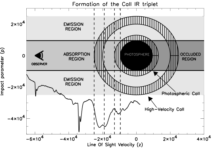
Figure 6 is a diagram of the formation of the CaII IR triplet feature in SN 2001el. The HVM has for illustration been shown as a spherical shell. The atmosphere can be divided into three regions, the high-velocity material in each region having a different affect on the spectrum. (1) The absorption region: Material in the tube directly in front of the photosphere absorbs photospheric light and emits line source function light into the line of sight. Since the line source function intensity is usually weaker than the photospheric intensity, this effect produces an absorption feature in the spectrum. (2) The emission region: material in the outer lobes does not obscure the photosphere but only adds line source function light; this produces an emission feature to the red of the absorption. (2) The occluded region: Material in the tube behind the photosphere is occluded by the photosphere and is not visible.
Because in our models it is the partial obscuration of polarized photospheric light that gives rise to the HVM polarization feature, all of our geometrical information on the HVM will be about the distribution of CaII in the absorption region. Whether there is any HVM CaII in the emission region, and if so, what its geometry may be, will be very difficult to say. In addition we will have absolutely no information about the material in the occluded region. In the spherical HVM shell of Figure 6, about 5% of the material is in the absorption region, 5% is in the occluded region, and 90% is in the emission region. Thus we only probe a small portion of the potential HVM. We now consider the general constraints of these regions in more detail.
4.1.1 Constraints on the Absorption Region Material
We can list 4 general constraints on the HVM absorption region material that are directly deducible from the Sept. 25 spectra:
(1) The width of the HVM flux absorption feature constrains to be non-zero only over the line-of-sight velocity range km s-1. is thus confined to a relatively thin region that is significantly detached from the photosphere. The edges of the flux feature are sharp, suggesting that the boundaries of the HVM are well-defined.
(2) At the minimum of the HVM absorption the flux has decreased by 43% from the continuum level. For geometries where the HVM covers the entire photosphere, the optical depth implied is . On the other hand, some geometries may have higher optical depths and smaller covering factors, the minimal covering factor being for when the lines are completely opaque. Note that in this context the term “covering factor” denotes the percent of the photospheric area obscured by the slice of HVM on a plane perpendicular to the line of sight, corresponding to the resonance surface of a certain wavelength. Since this differs from the traditional usage of the term, we hereafter call this the z-plane covering factor.
We can use the double-dipped flux profile to constrain the z-plane covering factor of the HVM. Because the 8542 blue triplet line is intrinsically stronger than the 8662 red triplet line (with a value 1.8 times larger), the blue minima of the IR triplet feature will be about twice as deep the red one unless both lines are saturated. Because the minima in the HVM feature are of about equal depth, we conclude that the two lines are indeed saturated (i.e. ) and the z-plane covering factor is in fact the minimal one, .
(3) The shape of the flux profile may also constrain the value . Note that two minima in the flux profile have roughly equal widths. On the other hand if all three triplet lines are saturated the blue minima will tend to be wider than the red, due to the blending of the with the line. This suggests that the line is weak while the other two lines are strong, a situation that occurs when .
(4) Finally, the HVM polarization feature points primarily in the u-direction. This means the distribution of the HVM is weighted along the line to the photosphere symmetry axis.
4.1.2 Constraints on the Emission Region Material
The material in the emission region may be observable as a flux emission feature to the red of the HVM absorption. If, for example, the HVM was a spherical shell, this emission feature would extend from about to , or over 1000 Å. The emission from a shell is then very broad, but because the line source function is much less than the photospheric intensity, the feature is typically weak and difficult to detect in the spectrum. A serious problem, evident from Figure 6, is that the HVM emission feature overlaps with the photospheric triplet absorption and emission, making it difficult to separate the two contributions. Only for the HVM material with (i.e. Å) is the HVM emission feature not blended with the photospheric. Unfortunately the available spectra of SN 2001el do not extend that far to the red.
The emission region material also affects the polarization level by diluting the photospheric light with unpolarized line source function light, thus creating a depolarization feature in the spectrum. Of course this depolarization feature gives no additional clue as to the orientation of the emission region material, as the unpolarized line light carries no directional information. The polarization spectrum of SN 2001el does have a significant depolarization to the red of the HVM peak, but since the overlapping photospheric triplet feature may also depolarize at these wavelengths, it is again not easy to use this to directly constrain the HVM emission region material. In our models, we do not attempt to fit the region redward of 8200 Å, where the HVM feature is blended with the photospheric feature.
We find that the red emission/depolarization feature is not a very sensitive diagnostic of emission region material. The effect on the spectrum is shown in Figure 7 for a spherical shell with various values of the destruction probability . For a pure scattering line () the emission is hardly visible. For the thermalized line () and a temperature , the emission would be substantial but difficult to separate from the photospheric component. A value is also unlikely for supernova atmospheres; NLTE models find .
The best way to constrain the amount of emission region material is by line of sight variations (see §5). The material in the emission region from one line of sight, becomes material in the absorption region from another. With a larger sample of supernovae one may be able to piece together a picture of the entire volume of high velocity ejecta.
4.2 Spherical Shell
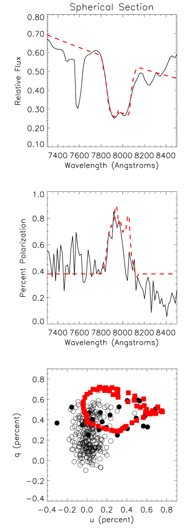
The first HVM geometry we consider is a spherically symmetric shell. We take the boundaries of the spherical shell to be km s-1 and km s-1 in order to reproduce the line width. Because the shell curves around, these dimensions actually give an extension in the z-direction of km s-1, consistent with constraint (1) of §4.1.1. The z-plane covering factor is found to be , and the optical depth necessary to fit the line depth .
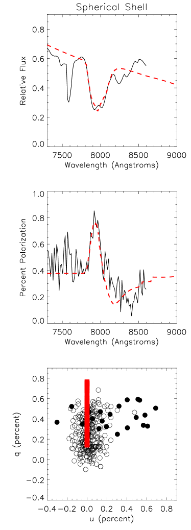
The triplet lines are not saturated in the spherical shell, so the model does not satisfy constraint (2) of §4.1.1 and will not well reproduce the flux profile. In Figure 8 we compare the synthetic spectra to the observed data. While the overall fit of the flux feature is decent, the redside minimum is not well reproduced. We will find better fits to the double-dipped profile using non-spherical geometries with smaller z-plane covering factors and saturated lines. Thus the flux spectrum alone suggests a deviation from spherical symmetry, although the evidence is rather subtle.
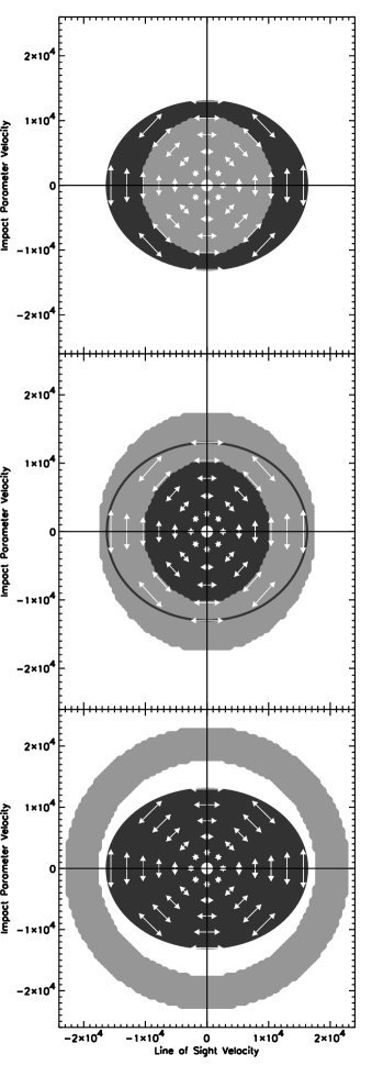
The effect of the spherical shell on the polarization is demonstrated by the slice plots of Figure 9. At the blue end of the absorption feature (slice a), the line obscures the weakly polarized, central light, allowing highly polarized, edge light to reach the observer. This creates a peak in the polarization spectrum. Further to the red of the feature (slice b), the line obscures the edge light and thus depolarizes the spectrum. Even further to the red (slice c), the line no longer obscures the photosphere, but the emission region material emits unpolarized line source function light into the line of sight, and a small level of depolarization continues. This polarization feature resembles an inverted P-Cygni profile, as discussed by Jeffrey (1989).
In Figure 8b we see that the spherical shell naturally reproduces the correct shape and size of the HVM polarization peak. The fact that the synthetic polarization feature has only a single peak is the result of a line blending effect: the red-side depolarization of the 8542 feature suppresses the peak due to the 8662 line. Note that while the observed depolarization minimum near 8400 Å is not well fit, this is not necessarily a weakness of the model. As discussed in §4.1.2 the feature at these wavelengths is produced mostly by the calcium near the photosphere, which has not been included in the model. In any case, the spherical shell, which follows the axial symmetry of the photosphere, does not change the polarization position angle as is observed (Figure 8c). This rules it out as a potential model for the HVM.
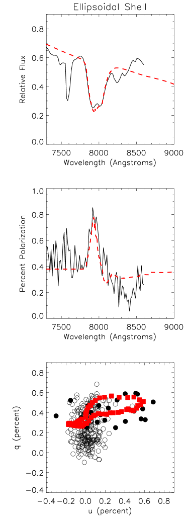
4.3 Rotated Ellipsoidal Shell
The good fit to the polarization level in Figure 8 suggests that a shell-like structure may be a viable candidate for the HVM, as long as the shell is somehow distorted from perfect spherical symmetry to account for the rotation of the HVM polarization angle. The simplest scenario is one where the HVM layers of the ejecta are ellipsoidal with the same oblateness as the photospheric layers, but with a rotated axis of symmetry. Exactly how such a relative rotation of the outer layers could arise from an SN Ia explosion is not obvious. One might envision that the rapid rotation of a white dwarf progenitor coupled with a deflagration to detonation transition at an off-center point (Livne, 1999) could produce something like this geometry.
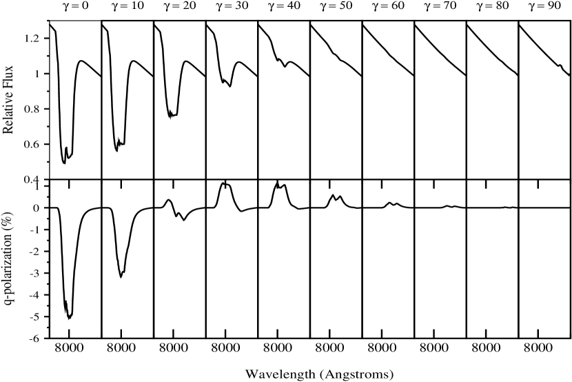
The effect of the rotated ellipsoidal shell on the polarization spectrum is demonstrated in the slice plots of Figure 10. The slices closely resemble those of the spherical shell (Figure 9) except that now the cross-sections of the HVM are ellipses. The shape and size of the flux and polarization features are thus very similar to the spherical case. For (HVM and photosphere axis aligned) the system is axially symmetric and the HVM polarization feature points in the q-direction. As is increased, the ellipses begin to absorb diagonally polarized light and the HVM polarization feature rotates into the u-direction.
The synthetic spectra for are shown in Figure 11. The ellipsoidal shell, like the spherical one, fails to meet constraint (2) and does not reproduce the double-dipped flux profile. This problem cannot be fixed by changing the ellipticity of the shell. On the other hand, the ellipsoidal shell is able to fit the polarization peak and the change of polarization angle.
Even more interestingly, the ellipsoidal shell produces a q-u loop similar to that observed in the data. In our models, we find that a q-u loop is a common signature of partial obscuration in two-axis systems. The absorption of the photospheric light typically produces a peak in both the q and u polarization. The partial obscuration effect on the q and u polarizations is distinct, so that in general these features do not peak at the same wavelength, but rather are out of phase. When plotted in the q-u plane, this phase offset makes a loop.
4.4 Clumped Shell
We parameterize a clumped shell as the section of the spherical shell lying within a cone of an opening angle (a “bowl” shaped structure, see Figure 4). A single clump like this could perhaps arise if the calcium in the HVM was produced by nuclear burning that occurred along a preferential axis. The clumped shell could also represent one piece of a shell broken into numerous clumps by an instability, a possibility discussed in more detail at the end of this section.
In deciding on the appropriate values for the clump parameters, we are guided by the constraints listed in §4.1.1. The opening angle is constrained to , so as to achieve the minimal z-plane covering factor (constraint 2). The orientation of the clump axis is chosen so that the clump lies in between the observer and the photosphere, obscuring the photosphere’s diagonal (constraint 4).
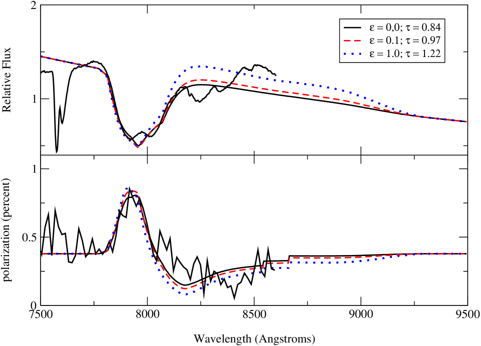
Through trial and error, a reasonable fit to the data was found for The synthetic spectra are shown in Figure 12. Because the lines are now saturated, the clump is able to reproduce the two equal minima of the flux absorption. The clumped shell also reproduces the important features of the polarization spectrum – i.e. the level of polarization, the polarization angle, and the q-u loop. On the other hand, the red edges of the synthetic flux and polarization spectra do not quite match the observed. In the polarization spectrum, the peak due to the 8662 feature is not suppressed by blending as it was in the shell models. This suggests that our parameterized clump geometry may be too simple and a more realistic model may involve a complicated superposition of clumps and shell.
In the geometry described above, the clump axis was chosen almost, but not quite, perpendicular to the photosphere axis (). One might wonder if the two axes could possibly be orthogonal (). Such a scenario is permissible if the clump axis remains at an angle to the line of sight and the whole system is rotated to be observed at an inclination . One might imagine this geometry as a blob of material that was ejected in the equatorial direction of the ellipsoidal photosphere.
Although our clumped shell model consists of only a single clump, it is possible that many more clumps exist in the emission region of the shell as the extra clumps would leave no obvious signature on the spectra (see §4.1.2). Clumpiness in a shell could be caused by various hydrodynamical instabilities. The expected scale of such clumpiness is unknown – it could perhaps take the form of a single large clump or it could be in the form of numerous smaller clumps. As we noted in reference to Equation 16 (see §3.5), the polarization feature due to partial obscuration is not sensitive to small scale structure, giving rather the integrated “moments” of the optical depth distribution. Thus we will not be able to empirically constrain the small scale structure of the clumpiness. We can say two things though: (1) Whatever the size of the clumps, their angular distribution must be weighted along the clump axis defined above. If the clumps were instead small structures distributed uniformly over the shell, when integrated up they would average out to the uniform spherical shell analyzed in the previous section, which did not show a rotation of the polarization angle. (2) This weighted angular distribution of the clumps cannot vary in the radial direction. If it did, the polarization angle of the HVM feature – which is set by however the randomly placed clumps happen to be distributed over the photosphere – would vary randomly across the HVM feature rather than forming a q-u loop oriented in the u-direction. Both of these suggest that the scale of the clumpiness is not much smaller than the single clump used in the model.
4.5 Toroid
A toroid would be an especially interesting structure to find in the ejecta of a SN Ia, as it might give a hint as to the binary nature of the progenitor system. In the currently preferred progenitor scenarios (see Branch et al. (1995)), SNe Ia are the result of a white dwarf accreting material either from the Roche-lobe overflow of a companion star or the coalescence with another C-O white dwarf. The orientation of the accretion disk axis naturally suggests an independent orientation of the outer ejecta layers, and this could provide a natural explanation why the HVM of SN 2001el deviates from the photospheric axis of symmetry.
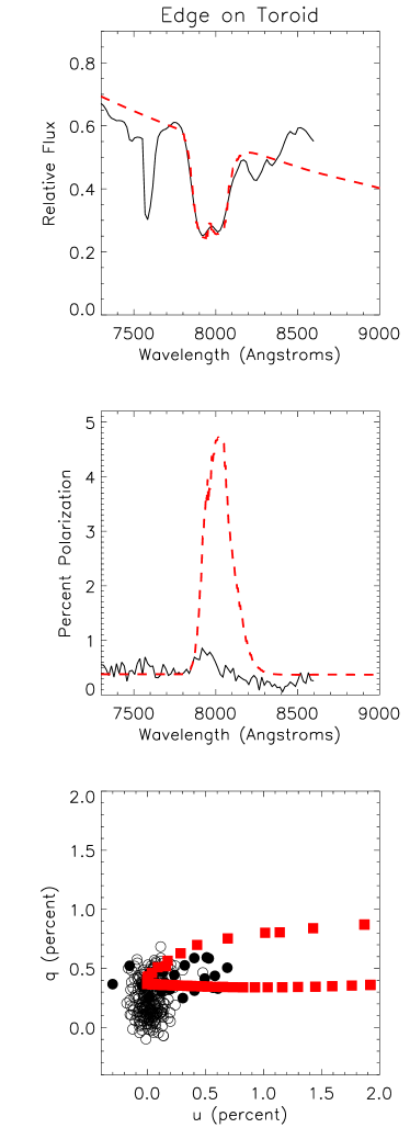
Whether an accretion disk could maintains a toroidal structure after the supernova explosion can only be addressed by multi-dimensional explosion modeling. Here we can calculate what effect such a structure would have on the flux and polarization spectrum, and whether it could possibly account for the HVM feature in SN 2001el. We parameterize the toroid as the ring of a spherical shell lying within opening angle (see Figure 4).
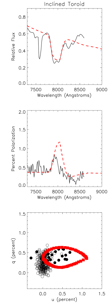
We first consider a system where the toroid is observed edge-on. We set , giving the minimal z-plane covering factor, and . We orient the torus axis at to preferentially absorb the diagonal light. The results are shown in Figure 13. The flux feature is a good match to the double-dipped profile, but the polarization peak at 5% is much too large. The reason is clear from the slice plot in Figure 14 – the edge-on toroid, which occludes opposite sides of the photosphere, is very effective at blocking light of a particular polarization.
A good fit to the polarization feature can still be sought by changing the inclination of the toroid. As the inclination is increased, the toroid rotates off the photodisk and both the flux and polarization feature decrease. The boundaries of the toroid and the opening angle must then be readjusted to properly fit the flux feature. In the present model a perfect fit cannot be found for any inclination. For all cases where the flux feature is well fit, the polarization feature is too strong. A compromise fit is shown in Figure 15. Here , , , and . The flux feature is too weak, and the polarization too strong.
5 The High Velocity Material from Other Lines of Sight
Previous discussions have pointed out that several different geometrical configurations are capable of providing reasonable fits to both the flux and polarization HVM features. The degeneracy problem is two-fold: (1) Different distributions of absorbing material in front of the photosphere can lead to similar polarization features (see the discussion in §3.5) (2) There is no strong diagnostic of the amount and distribution of material in the emission region (§4.1.2). In this section we consider how the degeneracy problem can be overcome by observing the HVM from multiple lines of sight.
One difficulty in exploring line of sight variations is that the number of possible configurations in a two-axis system is enormous. Even holding the boundaries of the HVM fixed, we still have as free parameters the angle between the photosphere and HVM symmetry axis and two angles specifying the line of sight. There is no easy way to catalog all the possibilities. Therefore to keep the discussion simple and general, in the following calculations we choose the underlying photosphere to be spherical. The HVM axis can then be aligned in the z-y plane (i.e. ), leaving as the only free parameter the inclination . The polarization is then in the q direction. Note that in light of Equation 3, a positive q-polarization indicates the net flux is vertically polarized, while a negative q-polarization indicates it is horizontally polarized.
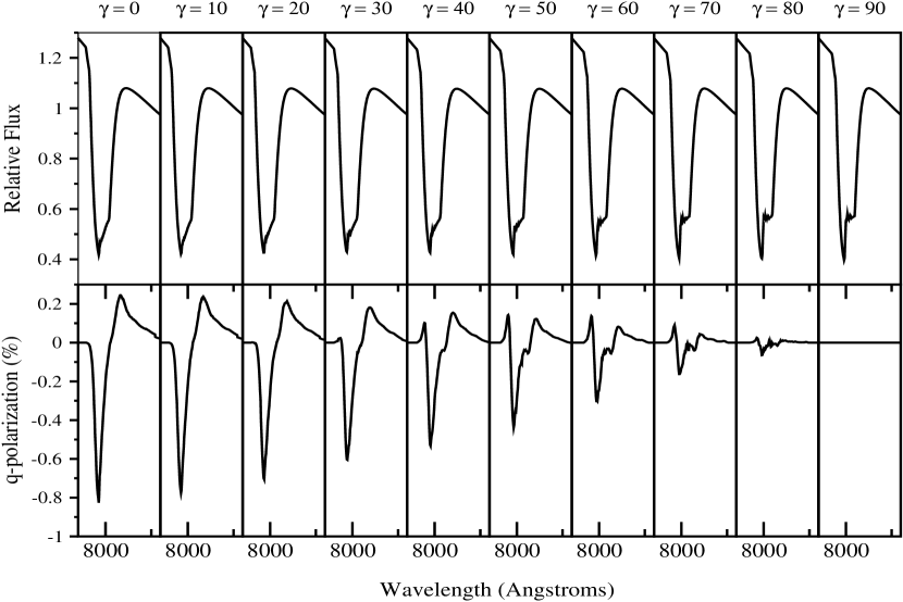
The ellipsoidal shell of §4.3 shows only subtle variations with inclination (Figure 16). A flux absorption is visible from all lines of sight, with the absorption profile barely changing with inclination. The only effect on the profile is a small shift of the minimum to the red as the short (i.e slow) end of the shell moves into the line of sight. For (shell viewed edge-on) the polarization is a maximum at 0.8%; this level is comparable to the HVM feature of SN 2001el. As is increased, the polarization feature decreases monotonically. For (shell viewed pole on) circular symmetry is recovered and the polarization is zero.
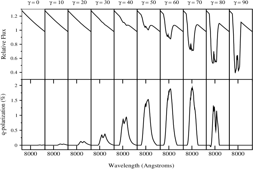
The clumped shell of §4.4, on the other hand, shows strong variations with inclination (Figure 17). The flux absorption is deepest for , when the clump is viewed top on, directly in between the photosphere and observer. At this inclination, the system is circularly symmetric and the polarization cancels (the perfect cancellation is of course the unnatural result of our simple “bowl-like” clump parameterization; a more irregularly shaped clump would show a small polarization feature). As is decreased, the clump moves to the edge of the photodisk, where it covers lower intensity, more highly-polarized light. As a result, the flux absorption gets weaker while the polarization feature becomes stronger. A strict inverse relationship holds for the inclinations and provides an important signature for the single clump model. For inclinations smaller than the polarization begins to decrease, but still remains much stronger than the flux feature. An especially striking signature occurs for the line of sight . Here the flux feature is barely visible while the polarization feature is strong (). The observation of this type of feature would clearly rule out an ellipsoidal shell and favor a single clump HVM geometry.
The variety of possible flux profiles from the clumped shell model correspond nicely to the variety of profiles that have already been observed in some other supernova. As the inclination is decreased from , the clump extends further in the z-direction – the two lines therefore become broader and the two minima more blended. When the clump is viewed directly on (), the two minima are largely resolved, which is not unlike the feature in SN 2001cx (Li et al., 2001). At slightly smaller inclinations () we found the best fits to the partially blended minima of SN 2001el. For the feature is weaker and the two minima are almost completely blended, resembling the rounded feature of SN 1990N (Leibundgut et al., 1991). For , the feature is very weak and about the depth that it was observed in SN 1994D (Meikle et al., 1996; Patat et al., 1996). Thus the clumped shell may be a single model capable of reproducing the full range of available observations on the HVM flux feature. More observations are necessary, however, to determine if the variety of flux profiles is indeed a line of sight effect or rather represents individual differences in the high velocity ejecta.
The most obvious signature of the toroidal geometry (Figure 18) is the high levels of polarization () when viewed near edge-on (). An edge-on toroid occludes vertically polarized light from the edges of the photosphere, giving a polarization feature with . As the toroid is inclined, the structure rotates off the photodisk and both the flux absorption and polarization peak weaken (in contrast to the clumped shell model). At inclinations greater than , the toroid begins to occlude the horizontally polarized light from the bottom of the photosphere – q then flips sign and becomes positive.
6 Summary and Conclusions
High quality spectropolametric observations of supernova may allow us to extract detailed information on the geometrical structure of the ejecta. Interpreting the polarization observations through modeling is a difficult endeavor, however, largely because of the the enormous number of configurations available in arbitrary 3-D geometries. The huge parameter space and multiple lines of sight make a direct comparison of data and first principle calculations difficult, not to mention computationally expensive. A parameterized approach is therefore useful in understanding the general polarization signatures arising from different geometrical structures. We have taken this approach here and calculated the polarization features expected from several geometries potentially relevant to SN 2001el.
The models computed in this paper highlight the wide range of spectropolametric features possible when aspherical geometries are considered. Depolarizing line opacity in the supernova atmosphere does not in general produce simple depolarization features in the polarization spectrum. Asymmetrically distributed line opacity often creates a polarization peak by partially obscuring the underlying photosphere. In systems where the line opacity follows a different axis of symmetry from the electron scattering medium, the resulting polarization feature generally creates a loop in the q-u plane. The two-component model described in this paper provides a convenient approach for quickly calculating and gaining intuition into the types polarization features arising from partial obscuration.
For the case of the high velocity material in type Ia supernova, partial obscuration will be a dominant effect on the line features, resulting in large polarization peaks (%) for practically any geometry considered. We have therefore explored to what extent partial obscuration alone can explain the CaII IR triplet polarization peak in SN 2001el. Our picture of the SN 2001el ejecta consists of nearly axially symmetric photospheric material surrounded by a detached, asymmetric structure at high velocity. We have investigated four possible geometries for the HVM: (1) A detached spherical shell is ruled out because it cannot account for the change of polarization angle over the HVM feature. The spherical shell also does not fit the shape of double-dipped flux absorption profile. (2) An ellipsoidal shell, with axis of symmetry rotated from the photosphere symmetry axis, can account for all the general features of the HVM polarization spectrum – the level of polarization, the polarization angle, and the q-u loop. However the ellipsoidal shell, like the spherical one, does not well fit the shape of the flux absorption profile. (3) A clumped shell, which could represent a single clump or a piece of a clumpy shell, can account for all the general features of the flux and polarization spectra. (4) A toroid, in the present model, produces a polarization feature that is larger than observed.
Different HVM geometries can be clearly discriminated by observing them from varying lines of sight. Depending upon the HVM geometry, a flux absorption similar to that of SN 2001el will be observed in SN Ia with different frequency. For a shell-like model, the flux signature will be observed from all lines of sight, while for the toroid and clump, only a fraction of the lines of sight produce the signature absorption. Under the assumption that the HVM has a similar structure in all (or at least a known subset) of SN Ia’s, it may be possible to constrain the geometry with a statistical sample of early flux spectra. Because the different models leave even more dramatic signatures on the polarization spectra, only a few well-observed supernova like SN 2001el are needed to discriminate the various scenarios (see §5).
We have not attempted in this paper to constrain the detailed geometry of the photospheric material. Because this material demonstrates a near axial symmetry, we have adopted the simple and general model of an edge-on oblate ellipsoid with a power law electron density profile. The actual photospheric geometry is likely more complicated, and may deviate from a strict axial symmetry. Given a more complicated photospheric structure, one could use the technique described here to calculate the HVM partial obscuration effect. Detailed monte-carlo studies on the structure of the photospheric material are under way; because the overall asymmetry of the photospheric material is rather small, however, our main conclusions about the HVM likely hold even when a more complicated photospheric geometry is used.
Although more observations are necessary to pin down the exact geometry of the HVM, one can begin to speculate as to its origin. Two questions in particular must be addressed: Why is the HVM feature geometrically detached from the photospheric material? And: Why does the HVM deviate from the dominant axis of symmetry of the photospheric material?
The detachment of the HVM indicates that the atmospheric conditions change rather suddenly at high velocity. Three possible changes (or a combination thereof) could result in an HVM feature (see Hatano et al. (1999)): (1) A spike in the overall density in the HVM: In the SN Ia deflagration model W7, the material at high velocity consists of unburnt carbon and oxygen with a solar abundance of calcium. The densities of these layers during the epoch in question are too low to produce an optically thick Ca II IR triplet. NLTE models (Nugent et al., 2002) show that – all other things being equal – a density increase at high velocity of more than an order of magnitude is necessary to produce an HVM feature. (2) A spike in the calcium abundance: For the W7 densities, the calcium abundance must be increased by from solar in order to produce an HVM feature (Nugent et al., 2002). This could, for example, be the result of blob of ejecta material that had undergone explosive oxygen burning, which increases the calcium abundance by (Khokhlov et al., 1993) (3) A sudden change in the ionization/excitation of the calcium: The optical depth of the IR triplet is a decreasing function of temperature (due to the increased ionization of Ca II to Ca III). Thus it is possible that a temperature decrease in the outer ejecta layers could make the IR triplet optically thick at high velocity. However it seems unlikely in this case that this optical depth spike would have sharp geometrical boundaries that persisted over several epochs of observations, as found for SN 2001el.
The distinct orientation of the HVM as compared to the photospheric material could be (1) the result of random processes in the explosion physics/hydrodynamics such as Raleigh-Taylor instabilities producing large scale clumpiness or (2) an indication of a preferred direction in the progenitor system. For example, the photospheric dominant axis could represent the rotation direction of the white dwarf while the HVM axis could represent the orientation of an accretion disk. Further explosion and hydrodynamical modeling is necessary to assess the plausibility of various scenarios.
References
- Branch et al. (1993) Branch, D., Fisher, A., & Nugent, P. 1993, AJ, 106, 2383
- Branch et al. (1983) Branch, D., Lacy, C. H., McCall, M. L., Sutherland, P. G., Uomoto, A., Wheeler, J. C., & Wills, B. J. 1983, ApJ, 270, 123
- Branch et al. (1995) Branch, D., Livio, M., Yungelson, L. R., Boffi, F. R., & Baron, E. 1995, PASP, 107, 1019
- Brown & McLean (1977) Brown, J. C. & McLean, I. S. 1977, A&A, 57, 141+
- Cassinelli & Haisch (1974) Cassinelli, J. P. & Haisch, B. M. 1974, ApJ, 188, 101
- Cassinelli & Hummer (1971) Cassinelli, J. P. & Hummer, D. G. 1971, MNRAS, 154, 9+
- Castor (1970) Castor, J. I. 1970, MNRAS, 149, 111
- Chandrasekhar (1960) Chandrasekhar, S. 1960, Radiative transfer (New York: Dover, 1960)
- Chugai (1992) Chugai, N. N. 1992, Soviet Astronomy Letters, 18, 168
- Code & Whitney (1995) Code, A. D. & Whitney, B. A. 1995, ApJ, 441, 400
- Cropper et al. (1988) Cropper, M., Bailey, J., McCowage, J., Cannon, R. D., & Couch, W. J. 1988, MNRAS, 231, 695
- Fisher et al. (1997) Fisher, A., Branch, D., Nugent, P., & Vaughan, T. 1997, ApJ, 481, 89
- Höflich et al. (2002) Höflich, P., Gerardy, C. L., Fesen, R. A., & Sakai, S. 2002, ApJ, 568, 791
- Hamilton (1947) Hamilton, D. R. 1947, ApJ, 106, 457
- Hatano et al. (1999) Hatano, K., Branch, D., Fisher, A., Baron, E., & Filippenko, A. V. 1999, ApJ, 525, 881
- Hillier (1994) Hillier, D. J. 1994, A&A, 289, 492
- Höflich (1991) Höflich, P. 1991, A&A, 246, 481+
- Höflich et al. (1996) Höflich, P., Wheeler, J. C., Hines, D. C., & Trammell, S. R. 1996, ApJ, 459, 307+
- Howell et al. (2001) Howell, D. A., Höflich, P., Wang, L., & Wheeler, J. C. 2001, ApJ, 556, 302
- Jeffery & Branch (1990) Jeffery, D. J. & Branch, D. 1990, in Supernovae, Jerusalem Winter School for Theoretical Physics, 149+
- Jeffrey (1989) Jeffrey, D. J. 1989, ApJS, 71, 951
- Jeffrey (1991) —. 1991, ApJ, 375, 264
- Khokhlov (1991) Khokhlov, A. 1991, A&A, 245, 114
- Khokhlov (2000) —. 2000, astro-ph/0008463
- Khokhlov et al. (1993) Khokhlov, A., Mueller, E., & Hoeflich, P. 1993, A&A, 270, 223
- Leibundgut et al. (1991) Leibundgut, B., Kirshner, R. P., Filippenko, A. V., Shields, J. C., Foltz, C. B., Phillips, M. M., & Sonneborn, G. 1991, ApJ, 371, L23
- Leonard et al. (2000) Leonard, D. C., Filippenko, A. V., Barth, A. J., & Matheson, T. 2000, ApJ, 536, 239
- Li et al. (2001) Li, W., Filippenko, A. V., Gates, E., Chornock, R., Gal-Yam, A., Ofek, E. O., Leonard, D. C., Modjaz, M., Rich, R. M., Riess, A. G., & Treffers, R. R. 2001, PASP, 113, 1178
- Livne (1999) Livne, E. 1999, ApJ, 527, L97
- Mahaffy & Hansen (1975) Mahaffy, J. H. & Hansen, C. J. 1975, ApJ, 201, 695
- Marietta et al. (2000) Marietta, E., Burrows, A., & Fryxell, B. 2000, ApJS, 128, 615
- McCall (1984) McCall, M. L. 1984, MNRAS, 210, 829
- Meikle et al. (1996) Meikle, W. P. S. et al. 1996, MNRAS, 281, 263
- Monard (2001) Monard, L. A. G. 2001, IAU Circ. No. 7720
- Nomoto et al. (1984) Nomoto, K., Thielemann, F., & Yokoi, K. 1984, ApJ, 286, 644
- Nugent et al. (2002) Nugent, P. et al. 2002, ApJ, in preparation
- Nugent (1997) Nugent, P. E. 1997, PhD thesis, University of Oklahoma
- Patat et al. (1996) Patat, F. et al. 1996, MNRAS, 278, 111
- Pinto & Eastman (2000) Pinto, P. A. & Eastman, R. G. 2000, ApJ, 530, 757
- Reinecke et al. (2002) Reinecke, M., Hillebrandt, W., & Niemeyer, J. 2002, A&A, in press
- Rybicki & Hummer (1978) Rybicki, G. B. & Hummer, D. G. 1978, ApJ, 219, 654
- Serkowski et al. (1975) Serkowski, K., Mathewson, D. L., & Ford, V. L. 1975, ApJ, 196, 261
- Shapiro & Sutherland (1982) Shapiro, P. R. & Sutherland, P. G. 1982, ApJ, 263, 902
- Stenflo (1994) Stenflo, J. O. 1994, Solar magnetic fields: polarized radiation diagnostics (Astrophysics and Space Science Library, Dordrecht; Boston: Kluwer Academic Publishers, —c1994)
- Thomas et al. (2002) Thomas, R. C., Kasen, D., Branch, D., & Baron, E. 2002, ApJ, 567, 1037
- Trujillo Bueno & Manso Sainz (1999) Trujillo Bueno, J. & Manso Sainz, R. 1999, ApJ, 516, 436
- Wang et al. (1997) Wang, L., Wheeler, J. C., & Hoeflich, P. 1997, ApJ, 476, L27
- Wang et al. (1996) Wang, L., Wheeler, J. C., Li, Z., & Clocchiatti, A. 1996, ApJ, 467, 435
- Wang et al. (2002) Wang, L. et al. 2002, ApJ, 1000, 1
- Wood et al. (1996) Wood, K., Bjorkman, J. E., Whitney, B. A., & Code, A. D. 1996, ApJ, 461, 828+
| Name | aa, : inner/outer radial or semi-major boundary in km s-1 | aa, : inner/outer radial or semi-major boundary in km s-1 | bb: Axis ratio | cc: optical depth of reference line () | dd: opening angle (see Figure 4) | ee: angles defining orientation of HVM symmetry axis (see Figure 4) | ee: angles defining orientation of HVM symmetry axis (see Figure 4) | fit-figure |
|---|---|---|---|---|---|---|---|---|
| spherical shell | 20,200 | 25,300 | 1.0 | 0.83 | - | - | - | 8 |
| ellipsoidal shell | 21,200 | 24,800 | 0.91 | 1.20 | - | 90∘ | 11 | |
| clumped shell | 20,600 | 24,300 | 1.0 | 5.0 | 12 | |||
| edge-on toroid | 20,900 | 24,500 | 1.0 | 5.0 | 13 | |||
| inclined toroid | 20,500 | 24,700 | 1.0 | 5.0 | 15 |