H$\delta$-Selected Galaxies in the Sloan Digital Sky Survey I: The Catalog

Abstract

We present here a new and homogeneous sample of 3340 galaxies selected from the Sloan Digital Sky Survey (SDSS) based solely on the observed strength of their H$\delta$  Hydrogen Balmer absorption line. The presence of a strong H$\delta$  line within the spectrum of a galaxy indicates that the galaxy has under–gone a significant change in its star formation history within the last Gigayear. Therefore, such galaxies have received considerable attention in recent years, as they provide an opportunity to study galaxy evolution in action. These galaxies are commonly known as “post–starburst”, “E+A”, “k+a” and H$\delta$–strong galaxies, and the study of these galaxies has been severely hampered by the lack of a large, statistical sample of such galaxies. In this paper, we rectify this problem by selecting a sample of galaxies which possess an absorption H$\delta$  equivalent width of ${\rm EW(H\delta_{\rm max})}-\Delta{\rm EW(H\delta_{\rm max})}>4$Åfrom 106682 galaxies in the SDSS. We have performed extensive tests on our catalog including comparing different methodologies of measuring the H$\delta$  absorption lines and studying the effects of stellar absorption, dust extinction and emission–filling on our measurements. We have determined the external error on our H$\delta$  measurements using duplicate observations of 11538 galaxies in the SDSS. The measured abundance of our H$\delta$–selected (HDS) galaxies is $2.6\pm 0.1$% of all galaxies within a volume–limited sample of $0.05<z<0.1$ and M($r^{*})<-20.5$, which is consistent with previous studies of such galaxies in the literature. We find that only 25 of our HDS galaxies in this volume–limited sample ($3.5\pm 0.7$%) show no, or little, evidence for [Oii]  and H$\alpha$  emission lines, thus indicating that true E+A (or k+a) galaxies (as originally defined by Dressler & Gunn) are extremely rare objects at low redshift, i.e., only $0.09\pm 0.02$% of all galaxies in this volume–limited sample are true E+A galaxies. In contrast, $89\pm 5$% of our HDS galaxies in the volume–limited sample have significant detections of the [Oii]  and H$\alpha$  emission lines. Of these, only 131 galaxies are robustly classified as Active Galactic Nuclei (AGNs) and therefore, a majority of these emission line HDS galaxies are star–forming galaxies. We find that $52\pm 12$% (27/52) of galaxies in our volume–limited HDS sample that possess no detectable [Oii]  emission, do however possess detectable H$\alpha$  emission lines. These galaxies may be dusty star–forming galaxies. We provide the community with this new catalog of H$\delta$–selected galaxies to aid in the understanding of these galaxies, via detailed follow–up observations, as well as providing a low redshift sample for comparison with higher redshift studies of HDS galaxies. We will study the global properties of these galaxies in future papers.

1 Introduction

The presence of a strong H$\delta$  absorption line (equivalent width of $\mathbin{\lower 3.0pt\hbox{$\,\hbox to0.0pt{\raise 5.0pt\hbox{$\char 62\relax$}\hss}\mathchar 29208\relax\,$}}5$Å) in the spectrum of a galaxy is an indication that the spectral energy distribution of that galaxy is dominated by A stars. Models of galaxy evolution indicate that such a strong H$\delta$  line (in the spectrum of a galaxy) can only be reproduced using models that include a recent burst of star formation, followed by passive evolution, as any on–going star–formation in the galaxy would hide the H$\delta$  absorption line due to emission–filling (of the H$\delta$  line) and the dominance of hot O and B stars, which have intrinsically weaker H$\delta$  absorption than A stars (see, for example, Balogh et al. 1999; Poggianti et al. 1999). Therefore the existence of a strong H$\delta$  absorption line in the spectrum of a galaxy suggests that the galaxy has under–gone a recent transformation in its star–formation history. In the literature, such galaxies are called “post–starburst”, “E+A”, k+a, and H$\delta$–strong galaxies and the exact physical mechanism(s) responsible for the abrupt change in the star formation history of such galaxies remains unclear. These galaxies have received much attention as they provide an opportunity to study galaxy evolution “in action”.

H$\delta$–strong galaxies were first discovered by Dressler & Gunn (1983, 1992) in their spectroscopic study of galaxies in distant, rich clusters of galaxies. They discovered cluster galaxies that contained strong Balmer absorption lines but with no detectable [Oii]  emission lines. They named such galaxies “E+A”, as their spectra resembled the superposition of an elliptical galaxy spectrum and A star spectrum. Therefore, E+A (or k+a) galaxies were originally thought to be a cluster–specific phenomenon and several physical mechanisms have been proposed to explain such galaxies. For example, ram–pressure stripping of the intra–stellar gas by a hot, intra–cluster medium, which eventually leads to the termination of star formation once all the gas in the galaxy has been removed, or used up (Gunn & Gott 1972; Farouki & Shapiro 1980; Kent 1981; Abadi, Moore & Bower 1999; Fujita & Nagashima 1999; Quilis, Moore & Bower 2000). Alternative mechanisms include high–speed galaxy–galaxy interactions in clusters (Moore et al. 1996, 1999) and interactions with the gravitational potential well of the cluster (Byrd & Valtonen 1990; Valluri 1993; Bekki, Shioya & Couch 2001).

To test such hypotheses, Zabludoff et al. (1996) performed a search for E+A (or k+a) galaxies in the Las Campanas Redshift Survey (LCRS; Shectman et al. 1996) and found that only 21 of the 11113 LCRS galaxies they studied, satisfied their criteria for a E+A galaxy. This work clearly demonstrates the rarity of such galaxies at low redshift. Furthermore, Zabludoff et al. (1996) found that 75% of their selected galaxies reside in the field, rather than the cores of rich clusters. This conclusion was confirmed by Balogh et al. (1999), who also performed a search for H$\delta$–strong galaxies in the redshift surveys of the Canadian Network for Observational Cosmology (CNOC; Yee, Ellingson, & Carlberg 1996), and found that the fraction of such galaxies in clusters was consistent with that in the field. Alternatively, the study of Dressler et al. (1999) found an order–of–magnitude increase in the abundance of E+A (or k+a) galaxies in distant clusters compared to the field (see also Castander et al. 2001). Taken together, these studies suggest that the physical interpretation of H$\delta$–strong galaxies is more complicated than originally envisaged, with the possibility that different physical mechanisms are important in different environment, e.g., 5 of the 21 E+A galaxies discovered by Zabludoff et al. (1996) show signs of tidal features, indicative of galaxy–galaxy interactions or mergers. Furthermore, redshift evolution might be an important factor in the differences seen between these surveys.

In addition to studying the environment of H$\delta$–strong galaxies, several authors have focused on understanding the morphology and dust content of these galaxies. This has been driven by the fact that on–going star formation in post–starburst galaxies could be hidden by dust obscuration (See Poggianti & Barbaro 1997; Poggianti et al. 1999; Bekki et al. 2001 for more discussion). In fact, Smail et al (1999) discovered examples of such galaxies using infrared (IR) and radio observations of galaxies in distant clusters. They discovered five post–starburst galaxies (based on their optical spectra) that showed evidence for dust–lanes in their IR morphology, as well as radio emission consistent with on–going star formation. However, radio observations of the Zabludoff et al. (1996) sample of nearby E+A galaxies indicates that a majority of these galaxies are not dust–enshrouded starburst galaxies. For example, Miller & Owen (2001) only detected radio emission from 2 of the 15 E+A galaxies they observed, and the derived star–formation rates (SFRs) were consistent with quiescent star formation and thus much lower than those observed for the dust–enshrouded starburst galaxies of Smail et al (1999). Chang et al. (2001) also did not detect radio emission from 5 E+A galaxies they observed from the Zabludoff et al. (1996) sample and concluded that these galaxies were not dust–enshrouded starbursts. In summary, these studies demonstrate that some E+A galaxies have dust–enshrouded star formation, but the fraction remains ill–determined. Furthermore, it is unclear how these different sub–classes of galaxies are related, and if there are any environmental and evolutionary processes at play.

The interpretation of H$\delta$–strong galaxies (E+A, k+a, etc.) suffers from small number statistics and systematic differences in the selection and definition of such galaxies between the different surveys constructed to date. Therefore, many of the difficulties associated with understanding the physical nature of these galaxies could be solved through the study of a large, homogeneous sample of H$\delta$  galaxies. In this paper, we present such a sample derived from the Sloan Digital Sky Survey (SDSS; York et al. 2000). The advantage of this sample, over previous work, is the quality and quantity of both the photometric and spectroscopic data, as well as the homogeneous selection of SDSS galaxies which covers a wide range of local environments.

We present in this paper a sample of galaxies that have been selected based solely on the observed strength of their H$\delta$  absorption line. Our selection is thus inclusive, containing many of the sub–classes of galaxies discussed in the literature until now, e.g., “E+A” or “k+a” galaxies (Zabludoff et al. 1996; Dressler et al. 1999), post–starburst galaxies, dust–enshrouded starburst galaxies (Smail et al. 1999), H$\delta$–strong galaxies (Couch & Sharples 1987) and the different subsamples of galaxies (i.e., e(a), A+em) discussed by Poggianti et al. (1999) and Balogh et al. (1999). Therefore, to avoid confusion with other samples in the literature, we simply call this sample of SDSS galaxies; “H$\delta$–selected” (HDS) galaxies.

In this paper, we present the details of our selection and leave the investigation and interpretation of these HDS galaxies to subsequent papers. We publish our sample of HDS galaxies to help the community construct larger samples of such galaxies, which are critically needed to advance our understanding of these galaxies, as well as aiding in the planning of follow–up observations and comparisons with higher redshift studies of such galaxies.

In Section 2, we present a brief discussion of the SDSS and the data used in this paper. In Section 3, we discuss our techniques for measuring the H$\delta$  absorption line and present comparisons between the different methodologies used to measure this line. In Section 4, we discuss the criteria used to select of our HDS sample of galaxies and present data on 3340 such galaxies in our catalog. In Section 5, we compare our sample of galaxies with those in the literature. A more detailed analysis of the properties of our HDS galaxies will be discussed in subsequent papers. The cosmological parameters used throughout this paper are ${\rm H_{0}}$=75 km s^-1 Mpc^-1, $\Omega_{m}=0.3$ and $\Omega_{\Lambda}=0.7$.

2 The SDSS Data

In this Section, we briefly describe the spectroscopic part of the SDSS. As discussed in York et al. (2000), the SDSS plans to obtain spectra for $\simeq 10^{6}$ galaxies to a magnitude limit of $r^{*}=17.7$ (the “Main” galaxy sample; Strauss et al. 2002), $\simeq 10^{5}$ Luminous Red Galaxies (LRG; Eisenstein et al. 2001) and $\simeq 10^{5}$ quasars (Richards et al. 2002). The reader is referred to Fukugita et al. (1996), Gunn et al. (1998), Lupton et al. (1999, 2001), York et al. (2000), Hogg et al. (2001), Pier et al. (2002), Stoughton et al. (2002), Smith et al. (2002) and Blanton et al. (2002a) for more details of the SDSS data and survey.

The SDSS spectra are obtained using two fiber-fed spectrographs (each with 320 fibers), with each fiber sub-tending 3 arcseconds on the sky. The wavelength coverage of the spectrographs is 3800Å to 9200Å, with a spectral resolution of 1800. The data from these spectrographs is automatically reduced to produce flux and wavelength–calibrated spectra (SPECTRO2D data analysis pipeline).

The SDSS spectra are then analyzed via the SDSS SPECTRO1D data processing pipeline to obtain a host of measured quantities for each spectrum (see Stoughton et al. 2002; Frieman et al., in prep, for further details). For example, SPECTRO1D determines the redshift of the spectrum both from absorption lines (via cross-correlation; Heavens 1993), and emission lines (via a wavelet–based peak–finding algorithm; see Frieman et al., in prep). Once the redshift is known, SPECTRO1D estimates the continuum emission at each pixel using the median value seen in a sliding box of 100 pixels centered on that pixel. Emission and absorption lines are then measured automatically by fitting of a Gaussian, above the best–fit continuum, at the redshifted rest–wavelength of expected lines. Multiple Gaussians are fit simultaneously for potential blends of lines (i.e., H$\alpha$  and [Nii]  lines). SPECTRO1D therefore provides an estimate of the equivalent width (EW), continuum, rest wavelength, identification, goodness–of–fit ($\chi^{2}$), height and sigma (and the associated statistical errors on these quantities) for all the major emission/absorption lines in these spectra. These measurements are done regardless of whether the line has been detected or not. For this work, we have used data from rerun 15 of the SPECTRO1D analysis pipeline, which is based on version 4.9 of the SPECTRO2D analysis pipeline (see Frieman et al. in prep for details of these pipelines).

For the sample of HDS galaxies presented in this paper, we begin with a sample of the SDSS galaxies that satisfy the following selection criteria:

1. Spectroscopically–confirmed by SPECTRO1D to be a galaxy;

2. Possess a redshift confidence of $\geq 0.7$;

3. An average spectroscopic signal–to–noise of $>5$ per pixel in the SDSS photometric $g$ passband;

4. z$\geq$0.05, to minimize aperture effects as discussed in Zaritsky, Zabuldoff & Willick (1995) and Gomez et al. (2003).

The reader is referred to Stoughton et al. (2002) for further details on all these SDSS quantities and how they are determined. After removing duplicate observations of the same galaxy (11538 galaxies in total; see Section 3.4), 106682 galaxies satisfy these criteria, up to and including spectroscopic plate 804 (observed on a Modified Julian Date of 52266 or 12/23/01; see Stoughton et al. 2002). Of these 106682 galaxies, it was only possible to measure the H$\delta$  line for 95479 galaxies (see Section 3.1 below) due to masked pixels at or near the H$\delta$  line. In Figure 1, we present the distribution of signal–to–noise ratios for all 106682 spectra (the median value of this distribution is 8.3).

Throughout this analysis, we have used the “smeared” SDSS spectra, which improves the overall spectrophotometric calibration of these data by accounting for light missed from the 3” fibers due to seeing and atmospheric refraction (see Gomez et al. 2003; Stoughton et al. 2002 for observational detail). Unfortunately, this smearing correction can systematically bias the observed flux of any emission and absorption lines in the spectrum, as the correction is only applied to the continuum. As shown by Hopkins et al. in prep., this is only a $\simeq 10\%$ effect on the flux of spectral lines, compared to using spectral data without the smearing correction applied. Furthermore, the equivalent width of our lines is almost unaffected by this smearing correction as, by definition, they are computed relative to the height of the continuum.

3 Spectral Line Measurements

3.1 H$\delta$ Equivalent Width

In this Section, we discuss the measurement of the equivalent width (EW) of the H$\delta$  absorption line in the SDSS galaxy spectra described in Section 2. The presence of a strong H$\delta$  absorption line in a galaxy spectrum indicates that the stellar population of the galaxy contains a significant fraction of A stars, which must have formed within the last Gigayear (see Section 1). The H$\delta$  line is preferred over other Hydrogen Balmer lines (e.g., H$\epsilon$, H$\zeta$, H$\gamma$, H$\beta$) because the line is isolated from other emission and absorption lines, as well as strong continuum features in the galaxy spectrum (e.g., D4000). Furthermore, the higher order Balmer lines (H$\gamma$ and H$\beta$) can suffer from significant emission–filling (see Section 3.3), while the lower order lines (H$\epsilon$ and H$\zeta$) are low signal–to–noise in the SDSS spectra.

In previous studies, several different methods have been employed to measure the H$\delta$  line, or select post–starburst galaxies. For example, Zabludoff et al. (1996) used the average EW of the H$\beta$ , H$\gamma$ and H$\delta$ lines to select E+A galaxies. Alternatively, Dressler et al. (1999) and Poggianti et al. (1999) interactively fit Gaussian profiles to the H$\delta$ line. Finally, Abraham et al. (1996), Balogh et al. (1999) and Miller & Owen (2002) performed a non–parametric analysis of their galaxy spectra, which involved summing the flux in a narrow wavelength window centered on each of the H$\delta$  line to determine the EW of the line. Castander et al. (2001) used an innovative PCA and wavelet analysis of spectra to select E+A galaxies. Each of these methods have different advantages and dis–advantages. For example, fitting a Gaussian to the H$\delta$  line is optimal for high signal–to–noise spectra, but can be prone to erroneous results when fit blindly to low signal–to–noise data or a weak absorption lines (such problems can be avoided if Gaussians are fit interactively; see Dressler et al. 1999; Poggianti et al. 1999). In light of the potential systematic differences between the different methods of measuring the H$\delta$  line, we have investigated the relative merits of the two main approaches in the literature – fitting a Gaussian and summing the flux in a narrow wavelength window – for determining the EW of the H$\delta$  line for the signal–to–noise, resolution, and size of the SDSS spectral dataset used in this paper.

First, we investigate the optimal method for computing the EW of the H$\delta$  line from the SDSS spectra using the non–parametric methodology outlined in Abraham et al. (1996) and Balogh et al. (1999), i.e., summing the flux within narrow wavelength windows centered on and off the H$\delta$ absorption line. We estimate the continuum flux via linear interpolation between two wavelength windows placed either side of the H$\delta$  line (4030Å to 4082Å and 4122Å to 4170Å). We used the same wavelength windows as in Abraham et al. (1996) and Balogh et al. (1999) for estimating the continuum because they are devoid of any strong emission and absorption features, and the continuum is relatively smooth within these wavelength ranges. Also, these windows are close to the H$\delta$  line without being contaminated by the H$\delta$  line emission. When fitting the continuum flux level, the flux in each pixel was weighted by the inverse square of the error on the flux in that pixel. After the initial fit to the continuum, we re–iterate the fit once by rejecting $3\sigma$ outliers to the original continuum fit. This guards against noise spikes in the surrounding continuum.

The rest–frame EW of the H$\delta$  line was calculated by summing the ratio of the flux in each pixel of the spectrum, over the estimated continuum flux in that pixel based on our linear interpolation. For this summation, we investigated two different wavelength windows for the H$\delta$  line; 4088Å to 4116Å, which is the same as the wavelength range used by Balogh et al. (1999) and 4082Å to 4122Å, which is the wider range of Abraham et al. (1996). We summarize the wavelength ranges used to measure the H$\delta$  EWs in Table 1.

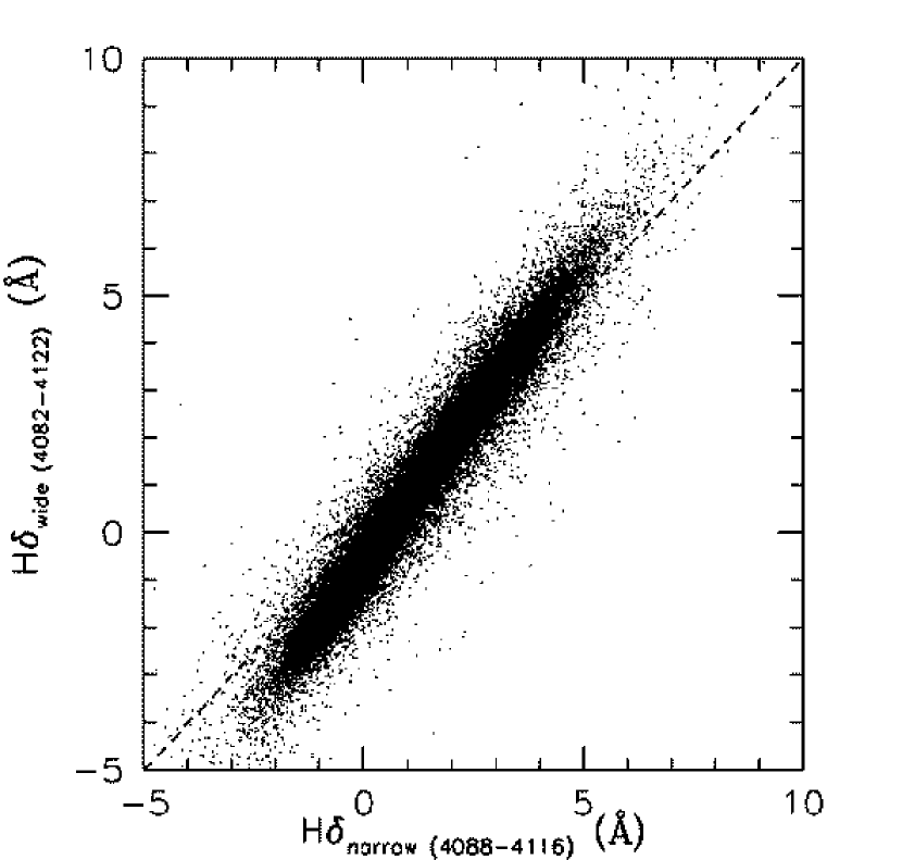
Figure 2: The H$\delta$  EW (Å) as measured in two different wavelength windows, i.e., the wide window of Abrahams et al. (1996) and the narrow window of Balogh et al. (1999). The expected one–to–one line is plotted to help guide the eye. For the work presented in this paper, absorption lines have a positive EW values and emission lines have negative EW values.

In Figure 2, we compare the two non–parametric measurements of H$\delta$ (i.e., using the narrow and wide wavelength windows), and find, as expected, a strong linear relationship between the two measurements: The scatter about the best fit linear relationship to these measurements is Gaussian with $\sigma=0.29$Å. However, there are systematic differences between the two measurements which are correlated to the intrinsic width of the H$\delta$  line. For example, for large EWs of H$\delta$, we find that the wider wavelength window has a larger value than the narrower window. This is because the 28Å window is too small to capture the wings of a strong H$\delta$  line and thus a wider window is needed. Alternatively, for smaller EWs, the narrower 28Å window is better as the larger window of 40Å is more affected by noise as it contains more of the continuum flux than the narrow window. This is seen in Figure 2 where the larger window systematically over–estimates the EW of the weaker H$\delta$  lines.

As a compromise, we have empirically determined that the best methodology for our analysis is to always select the larger of the two H$\delta$  EW measurements (this was discovered by visually inspecting many of the spectra and their various H$\delta$  measurements). This is a crude adaptive approach of selecting the size of the window based on the intrinsic strength of the H$\delta$  line. In fact, we find that 20.2% of our H$\delta$–selected galaxies (see Section 4) were selected based on the H$\delta$  measurement in the larger wavelength window. Therefore, for the analysis presented in this paper, we use H$\delta_{\rm max}$, which is the maximum of the two non–parametric measurements discussed above.

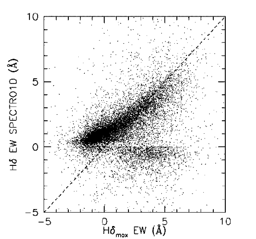
Figure 3: A comparison of the H$\delta$  EW as measured automatically by the SDSS SPECTRO1D spectroscopic pipeline (a Gaussian fit to the H$\delta$  line) and the non–parametric summation technique discussed in this paper and presented in Figure 2. The one–to–one line is shown to guide the eye. In our work, absorption lines have positive EW values and emission lines have negative EW values.

In Figure 3, we now compare the H$\delta_{\rm max}$ measurement discussed above to the automatic Gaussian fits to the H$\delta$  line from the SDSS SPECTRO1D analysis of the spectra. As expected, the two methods give similar results for the EW of the H$\delta$  line for the largest EWs. However, there are significant differences, as seen in Figure 3, between these two methodologies. First, there are many galaxies with a negative EW (emission) as measured by SPECTRO1D, but possess a (large) positive EW (absorption) using the non–parametric method. These cases are caused by emission–filling, i.e., a small amount of H$\delta$  emission at the bottom of the H$\delta$ absorption line (see Section 3.3). This results in SPECTRO1D fitting the Gaussian to the central emission line, thus producing a negative EW. On the other hand, the non–parametric method simply sums all the flux in the region averaging over the emission and still producing a positive EW. In Figure 4, we present five typical examples of this phenomenon.

Another noticeable difference in Figure 3 is the deviation from the one–to–one relation for H$\delta$  EWs near zero, i.e., as the H$\delta$  line becomes weak, it is buried in the noise of the continuum making it difficult to automatically fit a Gaussian to the line. In such cases, SPECTRO1D tends to over–estimate the EW of the H$\delta$  line because it preferentially fits a broad, shallow Gaussian to the noise in the spectrum. Typical examples of this problem are shown in Figure 5. We conclude from our study of the SDSS spectra that the non–parametric techniques of Abraham et al. (1996) and Balogh et al. (1999) are preferred to the automatic Gaussian fits of SPECTRO1D, especially for the lower signal–to–noise SDSS spectra which are a majority in our sample (see Figure 1). We note that many of the problems associated with the automatic Gaussian fitting of SPECTRO1D can be avoided by fitting Gaussians interactively. However, this is not practical for large datasets such as the SDSS.

3.2 [Oii]  and H$\alpha$  Equivalent Widths

In addition to estimating the EW of the H$\delta$  line, we have used our flux–summing technique to estimate the rest frame equivalent widths of both the [Oii]  and H$\alpha$  emission lines. We perform this analysis on all SDSS spectra, in preference to using the SPECTRO1D measurements of these lines, as these emission lines are the primary diagnostics of on–going star–formation in a galaxy and thus, we are interested in detecting any evidence of these lines in our HDS galaxies. As discussed in Section 3.1, the flux–summing technique is better for the lower signal–to–noise spectra, while the Gaussian–fitting method of SPECTRO1D is optimal for higher signal–to–noise detections of these emission lines, especially in the case of H$\alpha$  where SPECTRO1D de–blends the H$\alpha$  and [Nii]  lines.

We use the same flux–summing methodology as discussed above for the H$\delta$  line, except we only use one wavelength window centered on the two emission lines. We list in Table 1 the wavelength intervals used in summing the flux for the [Oii]  and H$\alpha$  emission lines and the continuum regions around these lines. Once again, the continuum flux per pixel for each emission line was estimated using linear interpolation of the continuum estimated either side of the emission lines (weighted by the inverse square of the errors on the pixel values during a line fitting procedure). We again iterate the continuum fit once rejecting $3\sigma$ outliers to the original continuum fit. We do not de–blend the H$\alpha$  and [Nii]  lines and as a result, some of our H$\alpha$  EW measurements may be over–estimated. However the contamination is less than 5% from [Nii]  line at 6648Å and less than 30% from [Nii]  line at 6583Å. We present estimates of the external error on our measurements of [Oii]  and H$\alpha$  in Section 3.4.

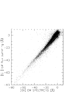
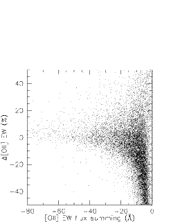
Figure 7: In the left panel, we present the comparison of our [Oii] EW measurements (flux summing) and those of SPECTRO1D (Gaussian fitting) for all SDSS spectra regardless of their H$\delta$ EWs. In the right panel, we plot the percentage difference between these two measurements. Positive percentages mean our flux summing method has a larger value.

In Figure 7, we compare our [Oii]  equivalent width measurements to that from SPECTRO1D for all SDSS spectra. In this paper, positive EWs are absorption lines and negative EWs are emission lines. There is a good agreement between the two methods for EW([Oii])$>10$Å, where the scatter is $\mathbin{\lower 3.0pt\hbox{$\,\hbox to0.0pt{\raise 5.0pt\hbox{$\char 60\relax$}\hss}\mathchar 29208\relax\,$}}10\%$. However, at lower EWs, the SPECTRO1D measurement of [Oii]  is systematically larger than our flux–summing method which is the result of SPECTRO1D fitting a broad Gaussian to the noise in the spectrum. Furthermore, our continuum measurements for the [Oii]  line are estimated close to the [Oii]  line, in a region of the spectrum where the continuum is varying rapidly with wavelength (e.g., D4000 break). Once again, we are only concerned with making a robust detection of any [Oii]  emission, rather than trying to accurately quantify the properties of the emission line. Therefore, we prefer our non–parametric method, especially for the low signal–to–noise cases.

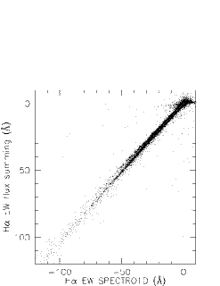
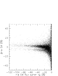
Figure 8: In the left panel, we present the comparison of our H$\alpha$ EW measurements (flux summing) and those of SPECTRO1D (Gaussian fitting) for all SDSS spectra regardless of their H$\delta$ EWs. In the right panel, we plot the percentage difference between these two measurements. Positive percentages mean our flux summing method has a larger value.

In Figure 8, we compare our H$\alpha$  equivalent width measurements against that of SPECTRO1D for all SDSS spectra regardless of their H$\delta$ EW. The two locii of points seen in this figure are caused by contamination in our estimates of H$\alpha$  due to strong emission lines in AGNs, i.e., the top locus of points have larger EWs in our flux–summing method than measured by SPECTRO1D due to contamination by the [Nii]  lines. This is confirmed by the fact that the top locus of points is dominated by AGNs. At low H$\alpha$  EWs, we again see a systematic difference between our measurements and those of SPECTRO1D, with SPECTRO1D again over–estimating the H$\alpha$  line because it is jointly fitting multiple Gaussians to low signal–to–noise detections of the H$\alpha$  and [Nii]  emission lines. Finally, we do not make any correction for extinction and stellar absorption on our flux–summed measurements of H$\alpha$(see Section 3.3).

3.3 Emission–Filling of the H$\delta$  Line

As mentioned above, our measurements of the H$\delta$  absorption line can be affected by emission–filling, i.e., H$\delta$  emission at the bottom of the H$\delta$  absorption line. This problem could be solved by fitting two Gaussians to the H$\delta$  line; one for absorption, one for emission. We found however that this method is only reliable for spectra with a signal–to–noise of $>20$ and, as shown in Figure 1, this is only viable for a small fraction of our spectra. Therefore, we must explore an alternative approach for correcting for this potential systematic bias; however, we stress that the sense of any systematic bias on our non–parametric summing method would be to always decrease (less absorption) the observed EW of the H$\delta$ absorption line and thus our technique gives a lower limit to the amount of H$\delta$  absorption in the spectrum.

To help rectify the problem of emission–filling, we have used the H$\alpha$  and H$\beta$ emission lines (where available) to jointly constrain the amount of emission–filling at the H$\delta$  line as well as estimate the effects of internal dust extinction in the galaxy. Furthermore, our estimates of the emission–filling are complicated by the effects of stellar absorption on the H$\alpha$  and H$\beta$ emission lines. In this analysis, we have used the SPECTRO1D measurements of H$\alpha$  and H$\beta$ lines in preference to our flux–summing technique discussed in Section 3.2, because the emission–filling correction is only important in strongly star–forming galaxies where the H$\alpha$  and H$\beta$ emission lines are well fit by a Gaussian and, for the H$\alpha$  line, require careful de–blending from the [Nii]  lines.

To solve the problem of emission–filling, we have adopted two different methodologies which we describe in detail below. The first method is an iterative procedure that begins with a initial estimate for the amount of stellar absorption at the H$\beta$ and H$\alpha$  emission lines, i.e., we assume EW (absorption) = 1.5Å and H$\alpha$ EW (absorption) = 1.9Å (see Poggianti & Barbaro 1997; Miller & Owen 2002). Then, using the observed ratio of the H$\alpha$  and H$\beta$ emission lines (corrected for stellar absorption), in conjunction with an attenuation law of $\tau=A\,\lambda^{-0.7}$ (Charlot & Fall 2000) for galactic extinction and a theoretical H$\alpha$  to H$\beta$ ratio of 2.87 (case B recombination; Osterbrock 1989), we solve for $A$ in the attenuation law and thus gain extinction–corrected values for both the H$\beta$ and H$\alpha$  emission lines. Next, using the theoretical ratio of H$\beta$ emission to H$\delta$  emission, we obtain an estimate for the amount of emission–filling (extinction–corrected) in the H$\delta$  absorption line. We then correct the observed H$\delta$  absorption EW for this emission–filling and, assuming the EW(H$\delta$) absorption is equal to EW(H$\beta$) absorption and EW(H$\alpha$) absorption is equal to 1.3 + $0.4\times$ EW(H$\beta$) absorption (Keel 1983), we obtain new estimates for the stellar absorption at the H$\alpha$  and H$\beta$ emission lines, i.e., where we begun the iteration. We iterate this calculation five times, but on average, a stable solution converges after only one iteration.

Our second method uses the D4000 break to estimate the amount of stellar absorption at H$\beta$, using EW(H$\beta$) $=-5.5\times\,{\rm D4000}+11.6$ (Poggianti & Barbaro 1997; Miller & Owen 2002). Then, assuming EW(H$\alpha$) absorption is equal to 1.3 + $0.4\times$ EW(H$\beta$) absorption, we obtain an measurement for the amount of stellar absorption at both the H$\alpha$  and H$\beta$ absorption lines. As in the first method above, we use the Charlot & Fall (2000) attenuation law, and the theoretical H$\alpha$  to H$\beta$ ratio, to solve for the amount of extinction at H$\alpha$  and H$\beta$, and then use these extinction–corrected emission lines to estimate the amount of emission–filling at H$\delta$. We do not iterate this method, as we have used the measured D4000 break to independently estimate the amount of stellar absorption at H$\beta$ and H$\alpha$.

We have applied these two methods to all our SDSS spectra, except for any galaxy that possesses a robust detection of an Active Galactic Nucleus (AGN) based on the line indices discussed in Kewley et al. (2002) and Gomez et al. (2003). For these AGN classifications, we have used the SPECTRO1D emission line measurements. We also stop our emission–filling correction if the ratio of the H$\beta$ and H$\alpha$  line becomes unphysical, i.e., greater than 2.87. By definition, the emission–filling correction increases our observed values of the H$\delta$  absorption line, with a median correction of 15% in the flux of the H$\delta$  absorption line. In Figure 6, we show the distributions of H$\delta$ emission EWs calculated using the two methods described above in a solid (iteration) and a dashed (D4000) line, respectively. It is re–assuring that overall these two methods give the same answer and have similar distributions.

3.4 External Errors on our Measured Equivalent Widths

Before we select our HDS sample of galaxies, it is important to accurately quantify the errors on our EW measurements. In our data, there are 11538 galaxies spectroscopically observed twice (see Section 2), which we use to quantify the external error on our EW measurements. In Figures 9, 10 & 11, we present the absolute difference in equivalent width of the two independent observations of the H$\delta$ , H$\alpha$  and [Oii]  lines, as a function of signal–to–noise. In this analysis, we have used the lower of the two measured signal–to–noise ratios (in SDSS $g$ band for H$\delta$  and H$\beta$, or $r$ band for H$\alpha$) as any observed difference in the two measurements of the EW will be dominated by the error in the noisier (lower signal–to–noise) of the two spectra. From this data, we determine the $1\sigma$ error for each line and assign this, as a function of signal–to–noise, to our EW measurements for each galaxy. We determine the sigma of the distribution by fitting a Gaussian (as a function of signal–to–noise) as shown in Figures 12, 13 & 14, and then use a 3rd order polynomial to interpolate between the signal–to–noise bins, thus obtaining the solid lines shown in Figures 9, 10 & 11. Using these polynomial fits, we can estimate the $1\sigma$ error on our EWs for any signal–to–noise. The coefficients of the fitted 3rd order polynomial for each line are given in Table 2.

In addition to quantifying the error on [Oii], H$\alpha$  and H$\delta$, we have used the duplicate observations of SDSS galaxies to determine the error on our emission–filling corrections. Only 400 (564) of the 11538 duplicate observations of SDSS galaxies have strong H$\alpha$  and H$\beta$ emission lines which are required for the iterative (D4000) method of correcting for emission–filling. The errors on the emission–filling correction are only a weak function of signal–to–noise, so we have chosen to use a constant value for their error, rather than varying the error as a function of the galaxy signal–to–noise as done for H$\delta$, [Oii]  and H$\alpha$  emission lines. One sigma errors on the emission correction of H$\delta$ for the iterative method (EF1) and the D4000 method (EF2) are 0.57Å and 0.4Å in EW, respectively.

4 A Catalog of HDS Galaxies

We are now ready to select our sample of HDS galaxies using the non-parametric measurements of the H$\delta$  EW (i.e., EW(H$\delta_{\rm max}$)). We begin by imposing the following threshold on EW(H$\delta_{\rm max}$);

$${\rm EW(H\delta_{\rm max})}-\Delta{\rm EW(H\delta_{\rm max})}>4\AA,$$ (1)

where $\Delta{\rm EW(H\delta_{\rm max})}$ is the $1\sigma$ error on H$\delta$  based on the signal–to–noise of the spectrum (see Figure 9). We have chosen this threshold ($4$Å) based on visual inspections of the data and our desire to select galaxies similar to those selected by other authors (Zabludoff et al. 1996; Balogh et al. 1999; Poggianti et al. 1999), i.e., galaxies with strong recent star formation as defined by the H$\delta$  line. This threshold (Eqn. 1) is applied without any emission–filling correction. For the signal–to–noise ratios of our spectra (Figure 1), only galaxies with an observed H$\delta$  of $\mathbin{\lower 3.0pt\hbox{$\,\hbox to0.0pt{\raise 5.0pt\hbox{$\char 62\relax$}\hss}\mathchar 29208\relax\,$}}5$Å satisfy Eqn. 1, which is close to the $5$Å threshold used by Balogh et al. (1999) to separate normal star–formating galaxies from post–starburst galaxies (see Figures 8 & 9 in their paper). Therefore, our HDS sample should be similar to those already in the literature, but is still conservative enough to be inclusive of the many different subsamples of H$\delta$–strong galaxies, like k+a, a+k, A+em and e(a), as discussed in Pogginati et al. (1999) and Balogh et al. (1999). We will present a detailed comparison of our HDS sample with models of galaxy evolution in future papers.

We call the sample of galaxies that satisfy Eqn. 1 “Sample 1”, and the sample contains 2526 galaxies from the main SDSS galaxy sample and 234 galaxies targeted for spectroscopy for other reasons, e.g., mostly because they were LRG galaxies (see Eisenstein et al. 2002), or some were targeted as stars or quasars (see Gordon et al. 2002).

We now apply the emission–filling correction for each galaxy to ${\rm EW(H\delta_{\rm max})}$ and select an additional sample of galaxies, that were not already selected in Sample 1 via Eqn 1, but now satisfy both the following criteria;

$${\rm EW(H\delta_{\rm max})}-\Delta{\rm EW(H\delta_{\rm max})}-\Delta{\rm EW(EF1)}>4\AA,\\$$ (2)

$${\rm EW(H\delta_{\rm max})}-\Delta{\rm EW(H\delta_{\rm max})}-\Delta{\rm EW(EF2)}>4\AA,$$ (2)

where $\Delta{\rm EW(EF1)}=0.57$Å and $\Delta{\rm EW(EF2)}=0.4$Å are the $1\sigma$ errors on the iterative method (EF1) and D4000 method (EF2) of correcting for emission–filling discussed in Section 3.4. Therefore, this additional sample of galaxies represents systems that would only satisfy the threshold in Eqn 1 because of the emission–filling correction (in addition to galaxies already selected as part of Sample 1). We call this sample of galaxies “Sample 2” and it contains 483 galaxies from the main SDSS galaxy sample and 97 galaxies which were again targeted for spectroscopy for other reasons, e.g., LRG galaxies, stars or quasars. On average, Sample 2 galaxies have strong emission lines because, by definition, they have the largest emission–filling correction at the H$\delta$  line. We have imposed both of these criteria to control the number of extra galaxies scattered into the sample. If we relaxed these criteria (i.e., remove both $\Delta{\rm EW(EF1)}$ and $\Delta{\rm EW(EF2)}$), then the sample would increase from 483 galaxies (in the main galaxy sample) to 1029. For completeness, we provide the extra 546 galaxies, which would be included if these criteria were relaxed, on our webpage.

In total, 3340 SDSS galaxies satisfy these criteria (Sample 1 plus Sample 2), and we present these galaxies as our catalog of HDS galaxies. We note that only 131 of these galaxies are securely identified as AGNs using the prescription of Kewley et al. (2002) and Gomez et al. (2003). In Figure 15, we present the fraction of HDS galaxies selected as a function of their signal–to–noise in SDSS $g$ band. It is re–assuring that there is no observed correlation, which indicates that our selection technique is not biased by the signal–to–noise of the original spectra.

For each galaxy in Samples 1 and 2, we present the unique SDSS Name (col. 1), heliocentric redshift (col. 2), spectroscopic signal–to–noise in the SDSS photometric $g$ band (col. 3), Right Ascension (J2000; col. 4) and Declination (J2000; col. 5) in degrees, Right Ascension (J2000; col. 6) and Declination (J2000; col. 7) in hours, minutes and seconds, the rest–frame EW(H$\delta$) (Å, col. 8), the rest–frame $\Delta$EW(H$\delta$) (Å, col. 9), the rest–frame EW([Oii]) (Å, col. 10), the rest–frame $\Delta$EW([Oii]) (Å, col. 11), the rest–frame EW(H$\alpha$) (Å, col. 12), the rest–frame $\Delta$EW(H$\alpha$) (Å, col. 13), the SDSS Petrosian $g$ band magnitude (col. 14), the SDSS Petrosian $r$ band magnitude (col. 15), the SDSS Petrosian $i$ band magnitude (col. 16), the SDSS Petrosian $z$ band magnitude (col. 17; all magnitudes are extinction corrected), the k–corrected absolute magnitude in the SDSS $r$ band (col. 18), SDSS measured seeing in $r$ band (col. 19), concentration index (col. 20, see Shimasaku et al. 2001 and Strateva et al. 2001 for definition). In Column 21, we present the AGN classification based on the line indices of Kewley et al. (2002), and in Column 22, we present our E+A classification flag, which is defined in Section 5.1. An electronic version of our catalog can be obtained at http://astrophysics.phys.cmu.edu/$\sim$tomo/ea.

In addition to presenting Samples 1 and 2, we also present a volume–limited sample selected from these two samples but within the redshift range of $0.05<z<0.1$ and with M$(r^{*})<-20.5$ (which corresponds to $r=17.7$ at $z=0.1$, see Gomez et al. 2003). We use Schlegel, Finkbeiner & Davis (1998) to correct for galactic extinction and Blanton et al. (2002b; v1_11) to calculate the k–corrections. In Table 3, we present the percentage of HDS galaxies that satisfy our criteria. In this table, the number of galaxies in the whole sample (shown in the denominator) changes based on the number of galaxies that could have had their H$\delta$, [Oii]  and H$\alpha$  lines measured because of masked pixels in the spectra.

We note here that we have not corrected our sample for possible aperture effects, except restrict the sample to $z\geq 0.05$: A 3 arcsecond fiber corresponds to $2.7h_{75}^{-1}$ kpc at this redshift, which is comparable to the half–light radius of most our galaxies (see also Gomez et al. 2003). We see an increase of $0.33$Å  ($\mathbin{\lower 3.0pt\hbox{$\,\hbox to0.0pt{\raise 5.0pt\hbox{$\char 60\relax$}\hss}\mathchar 29208\relax\,$}}10\%$) in the median observed H$\delta$ EW for the whole HDS sample over the redshift range of our volume–limited sample ($0.05<z<0.1$). This is probably caused by more light from the disks of galaxies going down the fiber at higher redshifts. We see no such trend for the subsample of true E+A galaxies (see Section 5) in our HDS sample.

5 Discussion

In this Section, we compare our sample of HDS galaxies against previous samples of such galaxies in the literature. Further analysis of the global properties (luminosity, environment, morphology, etc.) of these galaxies will be presented in future papers.

5.1 Comparison with Previous Work

In this Section, we present a preliminary comparison of our SDSS HDS galaxies with other samples of post–starburst galaxies in the literature. We have attempted to replicate the selection criteria of these previous studies as closely as possible, but in some cases, this is impossible. Furthermore, we have not attempted to account for systematic differences in the distribution of signal–to–noises, differences in the spectral resolutions, and differences in the selection techniques used by different authors, e.g., we are unable to fully replicate the criteria of Zabludoff et al. (1996) as we do not yet possess accurate measurements of the H$\gamma$ and H$\beta$ lines. Therefore, these are only crude comparisons and any small differences seen between the samples should not be over–interpreted until a more detailed analysis can be carried out. We summarize our comparison in Table 4 and discuss the details of these comparisons below: Table 4 does however, demonstrate once again the rarity of H$\delta$–strong galaxies, especially at low redshift, as well as illustrating the sensitivity of their detection to the selection criteria used.

We first compare our sample to that of Zabludoff et al. (1996), which is the most similar to our work, especially as the magnitude limits of the LCRS (used by Zabludoff et al. 1996) and the SDSS are close, thus minimizing possible bias. Zabludoff et al. (1996) selected E+A galaxies from the LCRS using the following criteria; a redshift range of $15,000<cz<40,000\,{\rm km\,s^{-1}}$, a signal–to–noise of $>8$ per pixel, an EW of [Oii]  of $>-2.5$Å, and an average EW for the three Balmer lines (H$\delta$, H$\gamma$ and H$\beta$) of $>5.5$Å. Using these four criteria, Zabludoff et al. (1996) selected 21 LCRS galaxies as E+A galaxies, which corresponds to 0.2% of all LCRS that satisfy the same signal–to–noise and redshift limits. We find 80 SDSS galaxies (from the whole SDSS dataset analyzed here) satisfy the same redshift range and [Oii] EW detection limit as used by Zabludoff et al. (1996), as well as having H$\delta$ EW of $>$5.5Å, which should be close to the average of the EW of the three Balmer lines (H$\delta$, H$\gamma$ and H$\beta$) used by Zabludoff et al. (1996). Of these 80 galaxies, 71 are in our HDS sample. Given all the caveats discussed above, it is re–assuring that we have found HDS galaxies at a similar frequency (see Table 4) as Zabludoff et al. (1996) and it suggests that our criteria are consistent.

Several other authors have used similar criteria to Zabludoff et al. (1996) to search for post–starburst galaxies in higher redshift samples of galaxies. For example, Fisher et al. (1998) used an average EW of the H$\delta$, H$\gamma$ and H$\beta$ lines of $>4$Å and an EW of [Oii]  of $<5$Å. With these criteria, they found 4.7% of their galaxies were E+A galaxies. Similarly, Hammer et al. (1997) used an average of H$\delta$, H$\gamma$ and H$\beta$ of $>5.5$Å, an EW of [Oii]  of $<$5–10 Å and $M_{B}<$-20 to select E+A galaxies from the CFRS field galaxy sample. They found that 5% of their galaxies satisfied these criteria.

We have also attempted to replicate the selection criteria of Dressler et al. (1999) and Balogh et al. (1999) as closely as possible, using all SDSS galaxies in the volume–limited sample with measured H$\delta$, [Oii]  and H$\alpha$, and not simply the HDS subsample. For example, the MORPHS collaboration of Dressler et al. (1999) and Poggianti et al. (1999) selected E+A galaxies using a H$\delta$  EW of $>3$ Å and an [Oii]  EW of $<5$Å . Using these criteria, they found a significant excess of E+A galaxies in their 10 high redshift clusters (21%), compared with the field region (6%). Alternatively, Balogh et al. (1999) selected E+A galaxies using H$\delta$  EW of $>5$Å and an [Oii]  EW of $<5$Å . They found instead $1.5\pm 0.8$% of cluster galaxies were classified as E+A galaxies compared to $1.2\pm 0.8$% for the field (brighter than M$(r)=-18.8+5{\rm log}h$ after correcting for several systematic effects).

In Table 4, we present a qualitative comparison of our HDS sample with these higher redshift studies and, within the quoted errors, the frequencies of HDS galaxies we observe are consistent with these works. However, we caution the reader not to over–interpret these numbers for several reasons. First, we are comparing a low redshift sample ($z<0.1$) of HDS galaxies to high redshift studies ($z\simeq 0.5$) of such galaxies, and we have not accounted for possible evolutionary effects or observational biases. In particular, we are comparing our sample against the corrected numbers presented by Balogh et al. (1999), which attempt to account for scatter in the tail of the H$\delta$  distribution due to the large intrinsic errors on H$\delta$  measurements, while Dressler et al. (1999) do not make such a correction. Secondly, we are comparing a field sample of HDS galaxies to predominantly cluster–selected samples of galaxies (were available, we only quote in Table 4 frequencies based on field samples). Finally, the luminosity limit of our volume–limited sample is brighter than the high redshift studies, which may account for some of the discrepancies.

Finally, we note that the original E+A phenomenon in galaxies, as discussed by Dressler & Gunn (1983, 1992), was defined to be a galaxy that possessed strong Balmer absorption lines, but with no emission lines, i.e., a galaxy with the signature of recent star–formation activity (A stars), but no indication of on–going star–formation (e.g., nebular emission lines). Given the quality of the SDSS spectra, we can re–visit this specific definition and select galaxies from our sample that possess less than $1\sigma$ detections of both the H$\alpha$  and [Oii]  emission lines, i.e., ${\rm EW([OII])+\Delta EW([OII])\geq 0}$Å  and ${\rm EW(H\alpha)+\Delta EW(H\alpha)\geq 0}$Å). We find that only $3.5\pm 0.7$% (25/717) of galaxies in the volume limited HDS sample satisfy such a strict criteria (see Table 3). We show example spectra of these galaxies in Figure 16 and highlight them in the catalog using the E+A classification flag. This exercise demonstrates that true E+A galaxies – with no, or little, evidence for on–going star–formation – are extremely rare at low redshift in the field, i.e., $0.09\pm 0.02$% of all SDSS galaxies in our volume–limited sample.

5.2 HDS Galaxies with Emission–lines

In this Section, we examine the frequency of nebular emission lines ([Oii], H$\alpha$) in the spectra of our HDS galaxies. This is possible because of the large spectral coverage of the SDSS spectrographs which allow us to study both the [Oii]  and H$\alpha$  emission lines for all galaxies out to a redshift of $\simeq 0.35$. We begin by looking at HDS galaxies that possess both the H$\alpha$  and [Oii]  emission lines. Using the criteria that both [Oii]  and H$\alpha$  lines must be detected at $>1\sigma$ significance (i.e., ${\rm EW([OII])+\Delta EW([OII])<0}$Å  and ${\rm EW(H\alpha)+\Delta EW(H\alpha)<0}$Å), we find that $89\pm 5$% (643/717) of HDS galaxies in our volume–limited sample are selected. Of these, 131 HDS galaxies possess a robust detection of an AGN, based on the line indices of Kewley et al. (2001), similar to the AGN plus post–starburst galaxy found recently in the 2dFGRS (see Sadler, Jackson & Cannon 2002). Therefore, a majority of these emission line H$\delta$  galaxies may have on–going star formation and are similar to the e(a) and A+em subsample of galaxies discussed by Poggianti et al. (1999) and Balogh et al. (1999). We show in Figure 17 examples of these HDS galaxies that possess both the [Oii]  and H$\alpha$  emission lines. The median SFR of these galaxies (calculated from H$\alpha$  flux, see Kennicut 1998) is $\simeq 0.5{\rm M_{\odot}/yr}$, with a maximum observed SFR of $50{\rm M_{\odot}/yr}$. We note that these SFRs have not been corrected for dust extinction or aperture effects, which could result in them being a factor of $5$ to $10$ lower than the true SFR for the whole galaxy (see Hopkins et al. in prep).

We next examine the frequency of HDS galaxies with [Oii]  emission, but no detectable H$\alpha$  emission. Using the criteria of EW(H$\alpha$) $<$1 $\sigma$ detection and EW([Oii]) $>$ 1$\sigma$ detection (i.e., ${\rm EW([OII])+\Delta EW([OII])<0}$Å  and ${\rm EW(H\alpha)+\Delta EW(H\alpha)\geq 0}$Å), we find $2.9\pm 0.65$% (21/717) of our HDS galaxies in the volume–limited sample satisfy these cuts. The presence of [Oii]  demonstrates that the galaxy may possess on–going star formation activity, yet the lack of the H$\alpha$  emission is curious. Possible explanations for this phenomena are strong self-absorption of H$\alpha$  by the many A stars in the galaxy and/or metallicity effect which could increase the [Oii]  emission relative to H$\alpha$  emission. We show several examples of these galaxies in Figure 18, and the lack of H$\alpha$  emission is clearly visible. The fact that many of these galaxies possess strong [Nii]  lines (flanking the H$\alpha$  line) indicates strong self–absorption is a likely explanation for the missing H$\alpha$  emission line. Median [OII] EW of these galaxies is 1.3 Å. Compared with 11.5 Åof HDS galaxies with both [OII] and H$\alpha$ emission, these galaxies have much lower amount of [OII] in emission.

Finally, we find that $3.8\pm 0.7$% (27/717) of our HDS galaxies in our volume–limited sample satisfy the following criteria; ${\rm EW([OII])+\Delta EW([OII])\geq 0}$Å  and ${\rm EW(H\alpha)+\Delta EW(H\alpha)<0}$Å. In comparison, only 52 of our HDS galaxies, the volume limited sample, have just no [Oii] emission detected (only EW([OII]) + $\Delta$ EW([OII]) $\geq$0Å). Therefore, 52$\pm$12% (27/52) of the galaxies with no detected [Oii], have detected H$\alpha$ emission. The existence of such galaxies has ramifications on high redshift studies of post–starburst galaxies, as such studies use the [Oii]  line to constrain the amount of on–going star–formation within the galaxies e.g., Balogh et al. (1999), Poggianti et al. (1999). Therefore, if the H$\alpha$  emission comes from star–formation activity, then these previous high redshift studies of post starburst galaxies may be contaminated by such galaxies. A possible explanation for the lack of [Oii]  emission is dust extinction e.g., Miller & Owen (2002) recently found dusty star–forming galaxies which do not possess [Oii]  in emission, but have radio fluxes consistent with on–going star formation activity. This explanation would also be consistent with the low signal–to–noise we observe in the blue–end of the SDSS spectra of these galaxies, relative to the signal–to–noise seen in the red–end of their spectra. Median H$\alpha$ EW of these galaxies are 1.5Å, whereas that of HDS galaxies with both [OII] and H$\alpha$ emission is 25.9Å.

6 Conclusions

We present in this paper the largest, most homogeneous, search yet for H$\delta$–strong galaxies (i.e., post–starburst galaxies, E+A’s, k+a’s, a+k’s etc.) in the local universe. We provide the astronomical community with a new catalog of such galaxies selected from the Sloan Digital Sky Survey (SDSS) based solely on the observed strength of the H$\delta$  Hydrogen Balmer absorption line within the spectrum of the galaxy. We have carefully studied different methodologies of measuring this weak absorption line and conclude that a non–parametric flux–summing technique is most suited for an automated application to large datasets like the SDSS, and more robust for the observed signal–to–noise ratios available in these SDSS spectra. We have studied the effects of dust extinction, emission–filling and stellar absorption upon the measurements of our H$\delta$  lines and have determined the external error on our measurements, as a function of signal–to–noise, using duplicate observations of 11358 galaxies in the SDSS. In total, our catalog of H$\delta$–selected (HDS) galaxies contains 3340 of the 95479 galaxies in the Sloan Digital Sky Survey (at the time of writing) and we present these HDS galaxies to the community to help in the understanding of such systems and to aid in the comparison with higher redshift studies of post–starburst galaxies.

The measured abundance of our H$\delta$–selected (HDS) galaxies is $2.6\pm$0.1% of all galaxies within a volume–limited sample of $0.05<z<0.1$ and M($r^{*}$)$<-20.5$, which is consistent with previous studies of post–starburst galaxies in the literature. We find that only 25 galaxies ($3.5\pm 0.7$%) of HDS galaxies in this volume limited sample show no, or little, evidence for [Oii]  and H$\alpha$  emission lines, thus indicating that true E+A galaxies (as originally defined by Dressler & Gunn) are extremely rare objects, i.e., only $0.09\pm 0.02$% of all galaxies in our volume–limited sample. In contrast, $89\pm 5$% of our HDS galaxies have significant detections of the [Oii]  and H$\alpha$  emission lines. Of these, 131 galaxies are robustly classified as Active Galactic Nuclei (AGNs) and therefore, a majority of these emission line HDS galaxies are star–forming galaxies, similar to the e(a) and A+em galaxies discussed by Poggianti et al. (1999) and Balogh et al. (1999). We will study the global properties of our HDS galaxies in further detail in future papers.

Figure 1: The distribution of signal–to–noise for spectra used in this analysis (see Section 2). The signal–to–noise presented here is the average signal–to–noise per pixel over the wavelength range defined by the SDSS photometric $g$ passband. The median signal–to–noise value is 8.3. Galaxies with signal–to–noise less than 5 were not used in our study.

Figure 4: Five typical examples of SDSS spectra with H$\delta$ emission filling. In such cases it is difficult to fit the H$\delta$ absorption emission with a single Gaussian due to a centrally peaked emission. The double hashed region of this figure, centered on the H$\delta$  line, represents the narrow wavelength window used to measure the EW of H$\delta$  as explained in Section 3.1. The slightly wider hashed region, again centered on the H$\delta$  line, represented the wide wavelength window used to measure the H$\delta$  line (see Section 3.1). Finally, the dashed regions, one on each side of the hashed regions, represents the wavelength regions used to estimate the continuum flux. See also Table 1 for details of the wavelength windows used on measuring the H$\delta$  line.

Figure 5: Five examples of noisy spectra where the SDSS SPECTRO1D pipeline has fit a broad absorption line, thus overestimating the H$\delta$  EW. The hashed regions are the same as presented and discussed in Figure 4.

Figure 6: The amount of emission filling correction of H$\delta$ EW. A solid line is for the iteration method (EF1) and the shaded histogram uses the D4000 method (EF2).

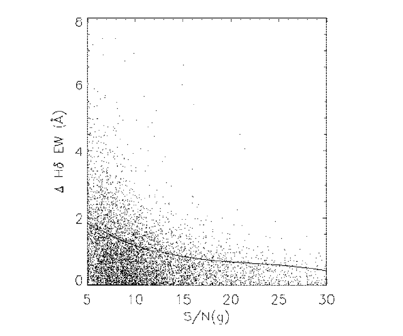
Figure 9: The absolute difference in the measured H$\delta$  EW (Å) for duplicate observations of SDSS galaxies as a function of signal–to–noise (the lower of the two signal–to–noise ratios has been plotted here). The solid line shows the $1\sigma$ polynomial line fitted to the distribution of errors (as a function of signal–to–noise).

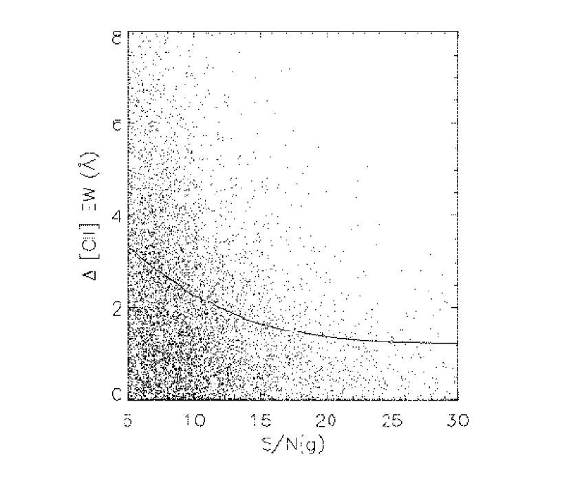
Figure 10: The absolute difference in the [Oii]  EW (Å) for duplicate observations of SDSS galaxies as a function of signal–to–noise (the lower of the two signal–to–noise ratios has been plotted here). The solid line shows the $1\sigma$ polynomial line fitted to the distribution of errors (as a function of signal–to–noise).

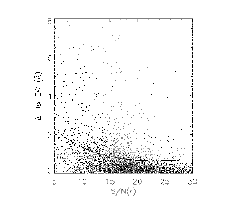
Figure 11: The absolute difference in the H$\alpha$  EW (Å) for duplicate observations of SDSS galaxies as a function of signal–to–noise (the lower of the two signal–to–noise ratios has been plotted here). The solid line shows the $1\sigma$ polynomial line fitted to the distribution of errors (as a function of signal–to–noise).

Figure 12: We present the distribution of differences for the H$\delta$  line from our duplicate observations. The four panels denote four different bins in signal–to–noise, i.e., clockwise from the top–left panel, we have s/n $<7$, $7<{\rm s/n}<10$, $15<{\rm s/n}<20$ and $10<{\rm s/n}<15$. We show as a dotted line the best fit gaussian to these distributions, which was then used to determine the $1\sigma$ error (shown for each panel) on H$\delta$  EW as a function of signal–to–noise.

Figure 13: We present the distribution of differences for the [Oii]  line from our duplicate observations. The four panels denote four different bins in signal–to–noise, i.e., clockwise from the top–left panel, we have $5<{\rm s/n}<10$, $10<{\rm s/n}<15$, $20<{\rm s/n}<25$ and $15<{\rm s/n}<20$. We show as a dotted line the best fit gaussian to these distributions, which was then used to determine the $1\sigma$ error on [Oii]  EW as a function of signal–to–noise.

Figure 14: We present the distribution of differences for the H$\alpha$  line from our duplicate observations. The four panels denote four different bins in signal–to–noise, i.e., clockwise from the top–left panel, we have $5<{\rm s/n}<10$, $10<{\rm s/n}<15$, $20<{\rm s/n}<25$ and $15<{\rm s/n}<20$. We show as a dotted line the best fit gaussian to these distributions, which was then used to determine the $1\sigma$ error on H$\alpha$  as a function of signal–to–noise.

Figure 15: The fraction of HDS galaxies as a function signal–to–noise in the $g$ band. The error bars are $\sqrt{N}$, where $N$ is the number of galaxies in each bin.

Figure 16: We show here five examples of spectra for the “true E+A” (k+a) subsample of HDS galaxies discussed in Section 5. These galaxies possess strong Balmer absorption lines, but have no, or little, detected [Oii]  or H$\alpha$  emission. We present a range of signal–to–noise ratios, as well as provide the measured redshift and H$\delta$  EW for each galaxy.

Figure 17: We present here five example spectra of our HDS galaxies that possess detected [Oii]  and H$\alpha$  emission lines. We present a range of signal–to–noise ratios, as well as provide the measured redshift and H$\delta$  EW for each galaxy.

Figure 18: We present here five example spectra of our HDS galaxies that possess detected [Oii]  emission lines, but no detected H$\alpha$. We present a range of signal–to–noise ratios, as well as provide the measured redshift, H$\delta$  EW and name for each galaxy.

Table 1: The wavelength ranges used to measure our H$\delta$, [Oii]  and H$\alpha$  EWs.

	Blue continuum	Line	Red continuum
H$\delta$ (narrow)	4030-4082Å	4088-4016Å	4122-4170Å
H$\delta$ (wide)	4030-4082Å	4082-4022Å	4122-4170Å
[Oii]	3653-3713Å	3713-3741Å	3741-3801Å
H$\alpha$	6490-6537Å	6555-6575Å	6594-6640Å

Table 2: Coefficients of third order polynomial fits to the error distributions shown in Figures 9, 10 and 11.

Line	a0	a1	a2	a3
H$\delta$	2.98	-0.28	0.012	-0.00018
[Oii]	4.96	-0.39	0.014	-0.00016
H$\alpha$	3.74	-0.36	0.014	-0.00017

Table 3: The frequency of finding HDS galaxies.

Category	% (All galaxies)	% (Volume Limited)
Whole HDS sample	3340/95479 (3.50$\pm$0.06%)	717/27014 (2.6$\pm$0.1%)
True “E+A”	140/94770 (0.15$\pm$0.01%)	25/26863 (0.09$\pm$0.02%)

Table 4: A comparison of our HDS sample of galaxies to previous work in the literature.

Author	Balmer lines	Emission	Their % (field)	Our %
Zabludoff et al.	H$\delta>$5.5Å	[OII]$>$-2.5Å	0.19$\pm$0.04%	0.16$\pm$0.02% (80/49994)
Poggianti et al.	H$\delta>$3 Å	[OII]$>$-5 Å	6$\pm$3%	5.79$\pm$0.15% (1565/27014)
Balogh et al.	H$\delta>$5 Å	[OII]$>$-5 Å	$1.2\pm 0.8$%	0.74$\pm$0.05% (200/27014)

References

- Abadi, Moore, & Bower (1999) Abadi, M. G., Moore, B., & Bower, R. G. 1999, MNRAS, 308, 947
- Abraham et al. (1996) Abraham, R. G. et al. 1996, ApJ, 471, 694.
- Balogh et al. (1999) Balogh, M. L., Morris, S. L., Yee, H. K. C., Carlberg, R. G., & Ellingson, E. 1999, ApJ, 527, 54.
- Bekki, Shioya, & Couch (2001) Bekki, K., Shioya, Y., & Couch, W. J. 2001, ApJ, 547, L17
- (5) Blanton, M.R., Lupton, R.H., Maley, F.M., Young, N., Zehavi, I., & Loveday, J. 2002a, AJ, submitted, astro-ph/0105535
- (6) Blanton, M. et al. 2002b, ApJ in press
- Byrd & Valtonen (1990) Byrd, G. & Valtonen, M. 1990, ApJ, 350, 89
- Castander et al. (2001) Castander, F. J. et al. 2001, AJ, 121, 2331
- Chang et al. (2001) Chang, T., van Gorkom, J. H., Zabludoff, A. I., Zaritsky, D., & Mihos, J. C. 2001, AJ, 121, 1965
- Charlot & Fall (2000) Charlot, S. & Fall, S. M. 2000, ApJ, 539, 718
- Couch & Sharples (1987) Couch, W. J. & Sharples, R. M. 1987, MNRAS, 229, 423
- Dressler & Gunn (1983) Dressler, A. & Gunn, J. E. 1983, ApJ, 270, 7
- Dressler & Gunn (1992) Dressler, A. & Gunn, J. E. 1992, ApJS, 78, 1
- Dressler et al. (1999) Dressler, A., Smail, I., Poggianti, B. M., Butcher, H., Couch, W. J., Ellis, R. S., & Oemler, A. J. 1999, ApJS, 122, 51.
- Eisenstein et al. (2001) Eisenstein, D. J. et al. 2001, AJ, 122, 2267
- Farouki & Shapiro (1980) Farouki, R. & Shapiro, S. L. 1980, ApJ, 241, 928
- Fisher, Fabricant, Franx, & van Dokkum (1998) Fisher, D., Fabricant, D., Franx, M., & van Dokkum, P. 1998, ApJ, 498, 195
- (18) Fukugita, M., Ichikawa, T., Gunn, J.E., Doi, M., Shimasaku, K., & Schneider, D.P. 1996, AJ, 111, 1748
- Fujita & Nagashima (1999) Fujita, Y. & Nagashima, M. 1999, ApJ, 516, 619
- (20) Gomez, P.L. et al. 2003, ApJ in press (see astro-ph/0210193)
- Gunn & Gott (1972) Gunn, J. E. & Gott, J. R. I. 1972, ApJ, 176, 1
- (22) Gunn, J.E., Carr, M.A., Rockosi, C.M., Sekiguchi, M., et al. 1998, AJ, 116, 3040
- Hammer et al. (1997) Hammer, F. et al. 1997, ApJ, 481, 49
- Heavens (1993) Heavens, A. F. 1993, MNRAS, 263, 735
- (25) Hogg, D.W., Schlegel, D.J., Finkbeiner, D.P., & Gunn, J.E. 2001, AJ, 122, 2129
- Keel (1983) Keel, W. C. 1983, ApJ, 269, 466
- Kennicutt (1998) Kennicutt, R. C. 1998, ApJ, 498, 541
- Kent (1981) Kent, S. M. 1981, ApJ, 245, 805
- Kewley et al. (2001) Kewley, L. J., Dopita, M. A., Sutherland, R. S., Heisler, C. A., & Trevena, J. 2001, ApJ, 556, 121
- (30) Lupton, R., Gunn, J. E., Ivezić, Z., Knapp, G. R., Kent, S., & Yasuda, N. 2001, in ASP Conf. Ser. 238, Astronomical Data Analysis Software and Systems X, ed. F. R. Harnden, Jr., F. A. Primini, and H. E. Payne (San Francisco: Astr. Soc. Pac.), p. 269 (astro-ph/0101420)
- (31) Lupton, R.H., Gunn, J.E., & Szalay, A.S. 1999, AJ, 118, 1406
- Miller & Owen (2001) Miller, N. A. & Owen, F. N. 2001, ApJ, 554, L25
- (33) Miller, N.A. & Owen, F.N. 2002, submitted to AJ
- Moore et al. (1996) Moore, B., Katz, N., Lake, G., Dressler, A., & Oemler, A. 1996, Nature, 379, 613
- Moore, Lake, Quinn, & Stadel (1999) Moore, B., Lake, G., Quinn, T., & Stadel, J. 1999, MNRAS, 304, 465
- Morris et al. (1998) Morris, S. L., Hutchings, J. B., Carlberg, R. G., Yee, H. K. C., Ellingson, E., Balogh, M. L., Abraham, R. G., & Smecker-Hane, T. A. 1998, ApJ, 507, 84
- (37) Osterbrock, D.E., 1989, Astrophysics of Gaseous Nebulae and Active Galactic Nuclei (University Science Books)
- (38) Pier, J.R., Munn, J.A., Hindsley, R.B., Hennessy, G.S., Kent, S.M., Lupton, R.H., & Ivezic, Z. 2002, AJ, submitted
- Poggianti & Barbaro (1997) Poggianti, B. M. & Barbaro, G. 1997, A&A, 325, 1025
- Poggianti et al. (1999) Poggianti, B. M., Smail, I., Dressler, A., Couch, W. J., Barger, A. J., Butcher, H., Ellis, R. S., & Oemler, A. J. 1999, ApJ, 518, 576
- Poggianti & Wu (2000) Poggianti, B. M. & Wu, H. 2000, ApJ, 529, 157.
- Quilis, Moore, & Bower (2000) Quilis, V., Moore, B., & Bower, R. 2000, Science, 288, 1617
- Richards et al. (2002) Richards, G. T. et al. 2002, AJ, 123, 2945
- Schlegel, Finkbeiner, & Davis (1998) Schlegel, D. J., Finkbeiner, D. P., & Davis, M. 1998, ApJ, 500, 525
- Shectman et al. (1996) Shectman, S. A., Landy, S. D., Oemler, A., Tucker, D. L., Lin, H., Kirshner, R. P., & Schechter, P. L. 1996, ApJ, 470, 172
- Shimasaku et al. (2001) Shimasaku, K. et al. 2001, AJ, 122, 1238
- Smail et al. (1999) Smail, I., Morrison, G., Gray, M. E., Owen, F. N., Ivison, R. J., Kneib, J.-P., & Ellis, R. S. 1999, ApJ, 525, 609
- (48) Smith, J.A., Tucker, D.L., Kent, S.M., et al. 2002, AJ, 123, 2121
- Stoughton et al. (2002) Stoughton, C. et al. 2002, AJ, 123, 485
- Strateva et al. (2001) Strateva, I. et al. 2001, AJ, 122, 1861
- (51) Strauss, M. et al. 2002, AJ in press
- Valluri (1993) Valluri, M. 1993, ApJ, 408, 57
- Yee, Ellingson, & Carlberg (1996) Yee, H. K. C., Ellingson, E., & Carlberg, R. G. 1996, ApJS, 102, 269
- York et al. (2000) York, D. G. et al. 2000, AJ, 120, 1579
- Zabludoff et al. (1996) Zabludoff, A. I., Zaritsky, D., Lin, H., Tucker, D., Hashimoto, Y., Shectman, S. A., Oemler, A., & Kirshner, R. P. 1996, ApJ, 466, 104
- Zaritsky, Zabludoff, & Willick (1995) Zaritsky, D., Zabludoff, A. I., & Willick, J. A. 1995, AJ, 110, 1602