Iterative techniques for the decomposition of long-slit spectra

Abstract

Two iterative techniques are described for decomposing a long-slit spectrum into the individual spectra of the point sources along the slit and the spectrum of the underlying background. One technique imposes the strong constraint that the spectrum of the background is spatially-invariant; the other relaxes this constraint. Both techniques are applicable even when there are numerous overlapping point sources superposed on a structurally-complex background. The techniques are tested on simulated as well as real long-slit data from the ground and from space.
Key words: instrumentation: spectrographs — methods: data analysis — techniques: spectroscopic

1 Introduction

Long-slit spectroscopy can be used to advantage in the investigation both of point sources and of extended emission. But for optimum results, reduction packages of some sophistication are required since the observed spectrum comprises the superposed spectra of all objects falling within the slit. Thus, for a point source, the spectrum of the underlying extended emission and the spectra of any nearby point sources need to be subtracted in order to extract the uncontaminated 1-D spectrum of the target. Correspondingly, for an extended object, the spectra of any superposed point sources must be subtracted in order to extract the uncontaminated 2-D spectrum of the target.

The subtraction tasks described above are clearly straightforward if the intensity of the extended emission has an approximately linear variation along the slit and if point sources are well separated. For such cases, standard IRAF procedures are applicable and not easily improved upon. But these same procedures must be expected to perform poorly when the observed field is not so simple. Accordingly, the aim of this investigation is to develop procedures for treating such cases. Examples which require more complex treatment include spectra of star clusters, planetary nebulae in Local Group Galaxies, H II regions in spiral arms, jets in young stars and galaxies, galactic nuclei and gravitational lenses.

Software that performs the above subtraction tasks in the more challenging circumstances where the extended emission is structurally complex and where the broadened spectra of point sources overlap are described and tested in this paper. Of course, given the errors associated with real data, no procedure can carry out these extraction tasks perfectly. Thus, some cross contamination will always remain in the extracted spectra of overlapping point sources as also between the extracted spectrum of a point source and that of the underlying extended emission. Nevertheless, procedures that perform such extractions with close to the optimum achievable reliability are clearly desirable.

Section 2 introduces two channel restoration in imaging and points out its relevance for the decomposition of long-slit spectra. Section 3 presents the iterative technique for a homogeneous background and section 4 for the general case of an inhomogeneous background. Section 5 presents simulations and applications of both methods to real data. As this investigation was underway, other authors have presented their treatments of essentially the same problem and a comparison between these various approaches is given in Section 6. The software implementation of the two new methods is briefly described in Section 7 and the conclusions in section 8.

2 Two channel restorations

The two iterative schemes for decomposing long-slit spectra, to be described in Sections 3 and 4, are variants of a previously-developed two-channel restoration procedure for astronomical images. Accordingly, we first recall salient aspects of this earlier work and identify an important innovation adopted here.

The problem of extracting reliable spectra of point sources and background from a long-slit spectrum is technically similar to that of achieving high photometric accuracy when restoring an image containing point sources superposed on extended emission. For this latter problem, Richardson-Lucy (RL) ((Richardson (1972), Lucy (1974)) or MaxEnt restorations are not satisfactory because of the ringing that occurs in the background close to the point sources.

Following earlier work by Frieden & Wells (1978), Hook & Lucy (1994b) and Lucy (1994) adopted a two channel approach to overcome this problem. All objects that the investigator deems to be point sources are allocated to one channel and all remaining emission to the second channel. The merit of this approach is that, rather than being presented with the impossible task of discovering delta functions from noisy and band-limited data, the restoration procedure is told which objects are to be restored as delta functions. Nevertheless, in order for the iterative procedure to find the desired solution, it also proves necessary to prevent the second channel from partially modelling the point sources as sharp peaks in the extended emission. This is accomplished by limiting the resolution of the second channel.

In the Lucy-Hook scheme (Hook & Lucy, 1994b), the angular resolution of $\psi$, the model of the extended emission, was limited by adding an entropic regularization term to the objective function to be maximized. This term penalizes differences between $\psi$ and $<\psi>$, the convolution of $\psi$ with an appropriate resolution kernel. Although effective, this procedure has the disadvantage of introducing a free parameter $\alpha$, the constant controlling the relative importance of the regularization term in the objective function. An implementation of the Lucy-Hook scheme for long-slit spectra has been described by Walsh (1997) and applied (Walsh, 2001).

In this paper, the required resolution limit is instead imposed by defining the restored background $\psi$ to be the convolution of a non-negative auxiliary function $\chi$ with a resolution kernel $R$. Clearly, $R$ itself then represents the narrowest feature that can appear in $\psi$. Accordingly, if the FWHM of $R$ exceeds that of the PSF, the convolution of $\psi$ with the PSF cannot fit the observed profile of a point source, which must therefore be modelled in the first channel as a delta function of appropriate amplitude.

As with images, an astronomer reducing a long-slit spectrum will often be confident in identifying some objects as point sources and will wish to benefit from the improved reduction that can result from providing such input.

3 Homogeneous background

The two techniques described in this paper differ only in their assumptions about the background. In this section, we make the strong, restrictive assumption that the background source is homogeneous. Thus, although the intensity of the background emission may vary along the slit, its spectrum does not. An example is a long-slit spectrum in the core of a globular cluster: numerous faint members then form a smooth background whose spectrum to a good approximation is spatially-invariant because of orbit-mixing.

3.1 Simplification

To simplify the description of the scheme, we assume that the observed spectrum $\tilde{\phi}(\lambda,y)$ is a continuous function of the two variables $\lambda$ and $y$, where $\lambda$ denotes wavelength and $y$ is the spatial coordinate perpendicular to the direction of dispersion. We further suppose that the spectra of the point sources have $\lambda$ -independent centroids $y_{n}$ - i.e., they are dispersed horizontally. Of course the actual code works with pixellated data and can correct for the curvature of the point-source spectra.

3.2 Model

Let $f_{n}(\lambda)$ be the spectrum of the $n$th point source and let $F(\lambda)$ be the spatially-invariant spectrum of the homogeneous background whose normalized spatial profile is $\psi(\eta)$. Then, if $P(y-\eta,\lambda)$ is the spatial distribution of a point source at $y=\eta$ due to instrumental broadening and seeing (for a ground-based telescope), the two- dimensional model for the observed spectrum is

$$\phi(\lambda,y)=F(\lambda)\theta(y,\lambda)+\sum_{n}f_{n}(\lambda)P(y-y_{n},\lambda)$$ (1)

where

$$\theta(y,\lambda)=\int\psi(\eta)P(y-\eta,\lambda)d\eta$$ (2)

is the broadenened and therefore $\lambda$-dependent profile of the background.

Now, as discussed in Sec. 2, the model as defined by Eqs. (1) and (2) is not yet satisfactory since a point source (especially one with a spectrum similar to that of the background) can be partially modelled as a peak in $\psi(\eta)$. To eliminate this near indeterminacy, we impose a resolution limit on $\psi$ by writing

$$\psi(\eta)=\int\chi(\zeta)R(\eta-\zeta)d\zeta$$ (3)

where $\chi(\zeta)$ is a non-negative normalized auxiliary function and $R(\eta-\zeta)$ is a non-negative normalized kernel function. If $R$ is a bell-shaped function with FWHM significantly greater than that of $P$, then point-like peaks cannot appear in $\psi(\eta)$. By thus preventing the point-sources from partially contaminating our model of the background, we simultaneously improve the accuracy of the extracted point-source spectra.

Eqs. (1)-(3) define the model used to decompose a long-slit spectrum under the assumption that the background is homogeneous. In fitting this model to an observed spectrum $\tilde{\phi}(\lambda,y)$, the unknowns to be estimated are the spectra $f_{n}(\lambda)$ and $F(\lambda)$ and the auxiliary function $\chi(\zeta)$. Note that the spatial profile of the background $\psi(\eta)$ is not a basic unknown but is obtained incidentally from $\chi(\zeta)$ via Eq.(3).

The point-spread function $P(y-\eta,\lambda)$ and the resolution kernel $R$ are user-supplied and thus treated as known functions in the iterative fitting procedure described below. The centroids $y_{n}$ of the point-source spectra are also user-supplied and are held fixed during the iterations. These $y_{n}$ can be input by the user or determined by cross-correlation with the point-spread function.

3.3 Iterative technique

We now estimate the unknown functions $f_{n}$, $F$ and $\chi$ by iteratively improving the fit of $\phi$ to the observed spectrum $\tilde{\phi}$. This iterative technique, which is based on the RL algorithm (Richardson 1972; Lucy 1974), alternates between improving the spectra $f_{n}(\lambda)$ and $F(\lambda)$ and improving the auxiliary function $\chi(\zeta)$.

The scheme is initiated with flat, featureless estimates for the unknown functions. Thus we take $f_{n}(\lambda)=F(\lambda)=1$ and set the normalized auxiliary function $\chi(\zeta)=1/Y$, where $Y$ is the spatial extent of the spectrum.

3.3.1 Correcting the spectra

After initiation (iteration $i=1$) or after a failed test of convergence ($i>1$), improved estimates of the spectra $f_{n}(\lambda)$ and $F(\lambda)$ are obtained as follows:

1) With the current estimate of the auxiliary function $\chi(\zeta)$, the profile of the background $\psi(\eta)$ is computed from Eq.(3).

Following this initial calculation, the remaining steps are carried out at each discrete $\lambda$ in the observed spectrum.

2) The broadened profile of the background $\theta(y,\lambda)$ is computed from Eq. (2).

3) With the current estimates of $f_{n}$ and $F$, the $y$-dependence of $\phi(\lambda,y)$ is derived from Eq. (1)

4) Improved values of the amplitudes $f_{n}$ are obtained by applying the correction factors

$$c_{n}=\int\frac{\tilde{\phi}(\lambda,y)}{\phi(\lambda,y)}P(y-y_{n},\lambda)dy$$ (4)

5) An improved value of $F$ is obtained by applying the correction factor

$$C=\int\frac{\tilde{\phi}(\lambda,y)}{\phi(\lambda,y)}\theta(y,\lambda)dy$$ (5)

When the above correction factors have been applied at all $\lambda$’s, the improved spectra are input to this iteration’s next stage - Sec.3.3.2 -wherein $\chi(\zeta)$ is improved.

3.3.2 Correcting the auxiliary function

Since the background is here assumed to have a spatially-invariant spectrum, the profile function $\psi(\eta)$ and the auxiliary function $\chi(\zeta)$ from which it is derived are $\lambda$-independent. In principle, therefore, these functions could be estimated from the data at a single $\lambda$, but at the price of then neglecting information at other $\lambda$’s. To avoid this, we project the model and the data onto the $y$-axis - i.e., we integrate over $\lambda$.

Let $\Phi(y)$ denote the integral of $\phi(y,\lambda)$. Then, from Eq.(1),

$$\Phi(y)=\Phi_{b}(y)+\sum_{n}\Phi_{n}(y)$$ (6)

where $\Phi_{b}(y)$ and $\Phi_{n}(y)$ are the corresponding integrals of the broadened background $F(\lambda)\theta(y,\lambda)$ and of the $n$th broadened point source $f_{n}(\lambda)P(y-y_{n},\lambda)$, respectively.

Now, using Eqs (1),(2) and (5), we can relate $\Phi_{b}(y)$ to the auxiliary function $\chi(\zeta)$. The result is the integral equation

$$\Phi_{b}(y)={\cal F}\int\chi(\zeta)Q(y-\zeta)d\zeta$$ (7)

where $\cal F$ denotes the integral of $F(\lambda)$ and

$$Q(y-\zeta)=\frac{1}{\cal F}\int\!\!\int F(\lambda)P(y-\eta,\lambda)R(\eta-\zeta)d\lambda d\eta$$ (8)

Note that $Q(y-\zeta)$ is a normalized non-negative function.

Having derived this basic integral equation, we can now describe the steps that result in an improved estimate for the auxiliary function $\chi(\zeta)$.

1) The effective broadening function $Q(y-\zeta)$ defined by Eq. (8) is computed.

2) The integrated model $\Phi(y)$ is computed from Eqs. (6) and (7).

3) An improved $\chi(\zeta)$ is obtained by applying the correction factor

$${\cal C}(\zeta)=\int\frac{\tilde{\Phi}(y)}{\Phi(y)}Q(y-\zeta)dy$$ (9)

where $\tilde{\Phi}(y)$ denotes the $\lambda$-integrated observed spectrum $\tilde{\phi}(\lambda,y)$.

When the above correction has been made, control moves to this iteration’s next stage wherein convergence is tested.

3.3.3 Test of convergence

As measures of the corrections made in Sec. 3.3.1 to the spectra, we compute

$$\delta_{n}=\int|\Delta f_{n}|d\lambda/\int f_{n}d\lambda$$ (10)

for each point source, and the corresponding quantity $\delta_{F}$ for the background. The symbol $\Delta$ is the difference in value between successive iterations.

Similarly, we assess the corrections made in Sec. 3.3.2 to the normalized function $\chi(\zeta)$ by computing the quantity

$$\delta_{\chi}=\int|\Delta\chi|d\zeta$$ (11)

If any of the quantities $\delta_{n}$, $\delta_{F}$ or $\delta_{\chi}$ exceeds an appropriately small quantity $\epsilon$, control returns to Sec. 3.3.1 in order to carry out the $(i+1)$-th iteration.

3.3.4 Output

If the above convergence test is satisfied, the reduction is finished and it remains only to output the quantities of scientific interest. These are the spectra $f_{n}(\lambda)$ and $F(\lambda)$ and the normalized profile of the background $\psi(\eta)$. For some problems, the spectra of some or all of the point sources will be of primary interest; in others, the spectrum of the background; in yet others, the spatial profile of the background.

In addition, the two-dimensional residual spectrum $\phi(\lambda,y)-\tilde{\phi}(\lambda,y)$ is computed and displayed. Ideally, these residuals will be entirely attributable to statistical fluctuations in the observed spectrum $\tilde{\phi}(\lambda,y)$. But if some residuals are significant, a flawed or incomplete reduction is indicated - see comment f) below. Of particular interest in this regard is the use of this residual spectrum to discover evidence that the background’s spectrum is not spatially-invariant and to identify the astrophysical source - e.g., nebular emission. Note that a weak departure from spatial invariance is likely to be less evident if the spectrum were reduced without this assumption (Sec. 4) and then such a departure sought by inspecting the two-dimensional background spectrum $F(\lambda,\eta)$ that is part of the output in the inhomogeneous case.

The auxiliary function $\chi(\zeta)$ is not part of the standard output. In particular, this function does not provide a better model of the background’s profile than does $\psi(\eta)$.

3.4 Comments

The following comments are intended to clarify various aspects of this iterative scheme:

a) The correction factors defined by Eqs. (4) and (5) are obtained from the RL algorithm by noting that the spectra $f_{n}(\lambda)$ and $F(\lambda)$ are spatially broadened into their respective contributions to the observed spectrum according to the functions $P(y-y_{n},\lambda)$ and $\theta(y,\lambda)$. Similarly, the correction factor defined by Eq. (9) follows from noting that $\chi(\zeta)$ is broadened into $\Phi_{b}(y)$ according to the function $Q(y-\zeta)$. Note that all these correction factors are unity if the model exactly matches the observed spectrum.

b) The scheme does not correct the extracted spectra $f_{n}(\lambda)$ and $F(\lambda)$ for instrumental broadening in the $\lambda$- direction, and thus they are not affected by deconvolution artifacts. Accordingly, the subsequent analysis of one of these point-source spectra can be carried out exactly as if it were the spectrum of an isolated point source extracted with a conventional package. Similarly, the spectrum of the background can be analysed as if the observation was of a source not contaminated by point sources.

c) In conventional applications of the RL algorithm, it is advisable to limit the number of iterations in order to avoid fitting statistical fluctuations in the data (Lucy 1974). Here this is prevented by the resolution limit imposed by the kernel $R$, and so the iterations can be continued to convergence.

d) In the software package, the unknown functions $f_{n}$, $F$ and $\chi$ are represented as finite vectors. The converged solution obtained with the above iteration scheme effectively determines the elements of these vectors from the Principle of Maximum Likelihood (Lucy 1974).

e) Statistical fluctuations in the extracted spectra $f_{n}(\lambda)$ and $F(\lambda)$ are not reduced by imposing a resolution limit in the $\lambda$-direction nor by restricting the number of iterations. Instead, noise in the $f_{n}$ is reduced by an effective weighted co-addition in the spatial direction using the broadening function $P(y-y_{n},\lambda)$ (cf Horne 1986; Robertson 1986). Similarly, noise in $F$ is reduced by an effective weighted co-addition using the broadening function $\theta(y,\lambda)$.

f) The model $\phi(\lambda,y)$ obtained with the above iterative scheme will not necessarily fit the observed spectrum $\tilde{\phi}(\lambda,y)$ to within errors. Significant residuals will remain if the assumptions underlying the model are violated. In particular, the background’s spectrum may not be spatially-invariant. Also the user-supplied broadening function $P(y-y_{n},\lambda)$ may be inaccurate.

Point sources not allocated to the first channel will also give significant residuals since, by design, the resolution kernel $R$ then prevents a close fit. In this case, a second reduction with additional designated point sources is clearly called for. A further cause of significant residuals would be a marginally-resolved source with FWHM less than that of $R$.

4 Inhomogeneous background

In this section, we relax the constraint that the background is homogeneous. Thus the general case is now treated where the background’s spectrum varies with position along the slit.

4.1 Model

If the background is inhomogeneous, its spectrum $F(\eta,\lambda)$ is not separable into the product $\psi(\eta)F(\lambda)$ as assumed in Sec. 3.2. Accordingly, in this case, the model for the two-dimensional spectrum is

$$\phi(\lambda,y)=\omega(\lambda,y)+\sum_{n}f_{n}(\lambda)P(y-y_{n},\lambda)$$ (12)

where

$$\omega(\lambda,y)=\int F(\lambda,\eta)P(y-\eta,\lambda)d\eta$$ (13)

is the broadened spectrum of the background.

Now, as in Sec. 3.2, we must prevent point sources from being partially modelled as peaks in $F(\lambda,\eta)$. To eliminate this possibility, we again impose a limit on the spatial resolution of the background by writing

$$F(\lambda,\eta)=\int\chi(\zeta,\lambda)R(\eta-\zeta)d\zeta$$ (14)

where $\chi(\zeta,\lambda)$ is a non-negative auxiliary function and $R(\eta-\zeta)$ is a non-negative normalized kernel function.

Eqs. (12)-(14) define the model used to decompose a long-slit spectrum of an inhomogeneous background with superposed point-sources In fitting this model to an observed spectrum $\tilde{\phi}(\lambda,y)$, the unknowns to be estimated are the spectra $f_{n}(\lambda)$ and the auxiliary function $\chi(\zeta,\lambda)$. The spatially-varying spectrum of the background $F(\lambda,\eta)$ is not a basic unknown but is obtained incidentally from the auxiliary function $\chi(\zeta,\lambda)$ via Eq.(14).

As in Sec. 3, the point-spread function $P(y-\eta,\lambda)$ and the resolution kernel $R$ are user-supplied, thus treated as known functions in the iterative fitting procedure described below, and the centroids $y_{n}$ of the point source spectra also remain fixed.

4.2 Iterative technique

We now estimate the unknown functions $f_{n}$ and $\chi$ by iteratively improving the fit of $\phi$ to the observed spectrum $\tilde{\phi}$. This iterative technique, which is again based on the RL algorithm, repeatedly sweeps through the spectrum improving both the spectra $f_{n}(\lambda)$ and the auxiliary function $\chi(\zeta,\lambda)$ until convergence is achieved.

The scheme is initiated with $f_{n}(\lambda)=1$ for all $n$ and with $\chi(\zeta,\lambda)=1$. In addition, the normalized effective broadening function

$$Q(y-\zeta,\lambda)=\int\!\!P(y-\eta,\lambda)R(\eta-\zeta)d\eta$$ (15)

that maps $\chi(\zeta,\lambda)$ into $\omega(\lambda,y)$ - see Eqs. (13) and (14) - is computed and stored for use during the iterations.

At each iteration, the following calculations are made at every discrete $\lambda$ in the observed spectrum:

1) The $y$-dependence of the broadened background $\omega(\lambda,y)$ is computed by convolving the current estimate of $\chi(\zeta,\lambda)$ with $Q(y-\zeta,\lambda)$.

2) The $y$-dependence of $\phi(\lambda,y)$ is computed from Eq.(12) using the current estimates of the amplitudes $f_{n}$.

3) Improved point-source amplitudes $f_{n}$ are obtained by applying the correction factors

$$c_{n}=\int\frac{\tilde{\phi}(y,\lambda)}{\phi(y,\lambda)}P(y-y_{n},\lambda)dy$$ (16)

4) The auxiliary function $\chi(\zeta,\lambda)$ is improved by applying the correction factor

$$C(\zeta,\lambda)=\int\frac{\tilde{\phi}(y,\lambda)}{\phi(y,\lambda)}Q(y-\zeta,\lambda)dy$$ (17)

4.2.1 Test of convergence

When steps 1)-4) have been carried out at all $\lambda$’s, convergence is tested. The quantities tested are $\delta_{n}$ as previously defined by Eq.(10) and $\delta_{\chi}$, which is redefined here as

$$\delta_{\chi}=\int\int|\Delta\chi|d\zeta d\lambda/\int\int\chi d\zeta d\lambda$$ (18)

If any of the $\delta_{n}$ or $\delta_{\chi}$ exceeds an appropriately small quantity $\epsilon$, control returns to step 1) above in order to carry out a further iteration.

4.2.2 Output

If the above convergence test is satisfied, the reduction is finished and it remains only to output the quantities of scientific interest. These are the spectra of the point sources $f_{n}(\lambda)$ and the two-dimensional spectrum of the background $F(\lambda,\eta)$. This latter quantity is computed from the converged auxiliary function $\chi$ via Eq.(14).

From $F(\lambda,\eta)$, one-dimensional plots of the background spectrum at different positions $\eta$ along the slit can be displayed. Alternatively, one-dimensional plots of the background’s spatial profile at different $\lambda$’s can be extracted.

As in the homogeneous case, the two-dimensional residual spectrum $\phi(\lambda,y)-\tilde{\phi}(\lambda,y)$ is also computed and displayed. If some residuals are statistically significant, a flawed or incomplete reduction is indicated - see comment b) below.

4.3 Comments

The following comments refer to differences between this iteration scheme and that of Sec. 3.

a) Statistical fluctuations in the extracted background spectrum $F(\lambda,\eta)$ are reduced by an effective weighted co-addition in the spatial direction using the broadening function $Q(y-\zeta,\lambda)$ given by Eq. (15).

b) The converged model $\phi(\lambda,y)$ obtained with the above iterative scheme will not necessarily fit the observed spectrum $\tilde{\phi}(\lambda,y)$ to within errors. But significant residuals are less likely than in the previous case because the restrictive assumption of a spatially-invariant background spectrum has been dropped. Nevertheless, as previously, significant residuals will remain if the user-supplied broadening function $P(y-y_{n},\lambda)$ is inaccurate, if the second channel still contains point-sources, or if the background contains structure or resolved sources with widths narrower than that of $R$.

5 Applications

The two techniques are distinguished by their treatment of the extended source. If the spectrum of the extended source changes with spatial position across the slit, then the inhomogeneous technique should be applied; if the spectrum of the extended source is expected not to vary with position then the homogeneous code is applicable and will give a more robust estimation for the extended source with incidental improvements in the extracted spectra of the point sources.

The capabilities are illustrated by Figure 1 which shows a simulated 2D spectrum and the results of extraction of the point source spectra using the inhomogeneous technique (Sect. 4). The extended source consists of two spectral components with differing spatial extents - one with a sloping background and the other with line emission. The point sources have respectively a continuum with an absorption line and a flat continuum with emission lines. The difference in the continua of the two point sources is 1.75mag. at the short wavelength end of the spectrum. The results for the restored spectrum are shown: the match of the restored extracted point source spectra (integrated over the spatial extent) and the input templates are excellent. The difference between the restored long-slit spectrum (point and extended sources) and the input shows only random noise and no systematics, validating, in practice, the techniques described in Section 4.

In reality, the spectrum of the PSF (hence called the Slit Spread Function SSF) is often not a perfect match to the data because of instrumental effects and changing seeing (for ground-based data); the exact position of the point source(s) (required to shift the SSF to the position of a point source) are also not known. Ideally a PSF star should be placed on the slit together with the target, or, in the case of mulit-slit instruments, on another slitlet. However even having a star on the slit is not a guarantee of a good SSF. Experiments with ground-based data on a visual binary with separation $\leq$ seeing, using an SSF derived from a star at the edge of the slit, resulted in systematic residuals of the restoration which were spectrally varying. Thus the SSF at the edge of the slit was not identical to that at the centre on account of optical aberrations in the spectrometer. For HST spectra taken with STIS, for example, a spectrum of a point source at approximately the same position on the slit as the source could be used for the SSF. However very often suitable stars have lower signal-to-noise than the target or were not similarly centred in the slit. In addition two HST SSF’s may not be identical because of ”breathing” (thermally induced changes in the telescope focal length), particularly if the exposure times differ greatly between the object and SSF star.

In the case of space-based or adaptive optics long-slit spectra, the SSF can be constructed from an optical model, such as TinyTim for HST (Krist, 1995). Tiny Tim delivers a monochromatic PSF or a PSF integrated over a filter passband. Integrating the PSF with a slit of the correct size and pixel sampling allows a monochromatic long-slit PSF to be formed. Interpolating several such across the wavelength range of a long-slit spectrum allows construction of a high fidelity SSF image. In order to obtain the utmost from the slit spectra to be decomposed, precuations should be taken at the time of observation, or even at the time of instrument design in the case of a specialized instrument.

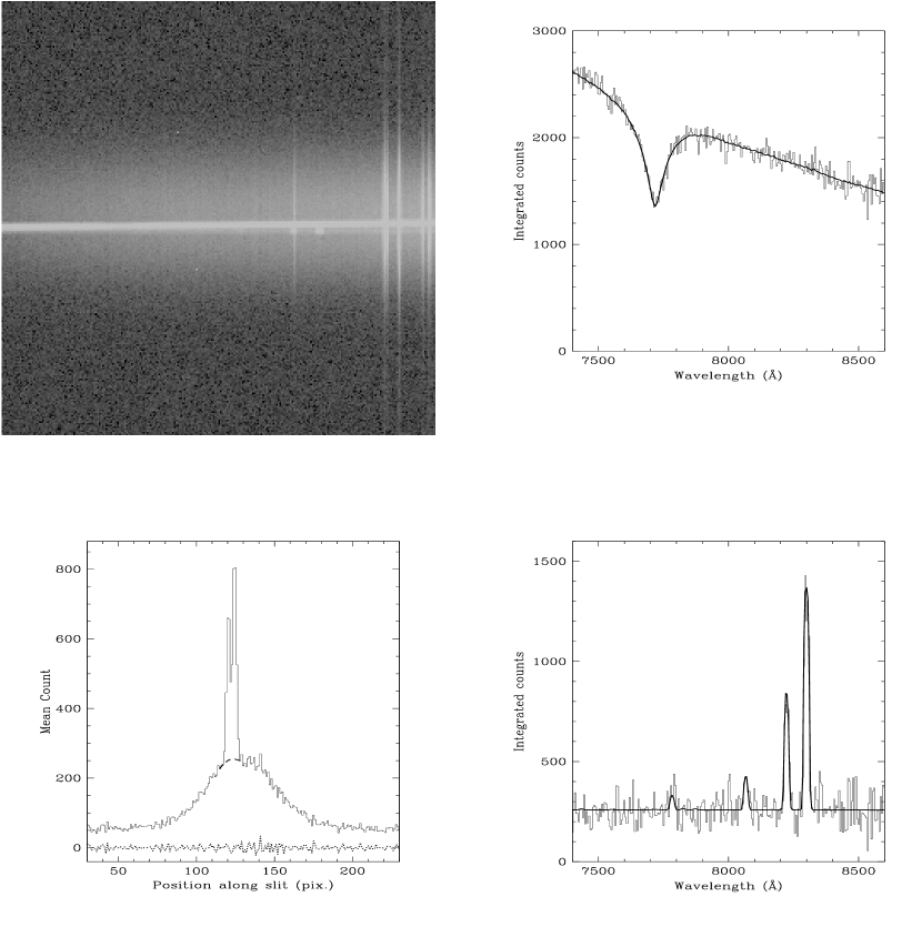
Figure 1: The capabilities of the inhomogeneous technique are illustrated by a simulated 2D spectrum (dispersion in X direction), shown at upper left, consisting of two point sources, of FWHM 2.7pixels separated by 1.3 times their width. The upper point source has a continuous spectrum with a broad absorption line (upper right) and the lower one emission lines on a flat continuum (lower right). The extended source is a broad Gaussian whose spectrum consists of a sloping continuum and emission lines with different spatial profiles. An arbitrary wavelength scale has been applied to the X axis and Gaussian distributed random noise was added. The 2D spectrum was restored with the inhomogeneous code (Sect. 4) and the restored point source spectrum (histogram) is compared with the input spectrum (bold line) in the right hand plots for both sources; the spectra are integrated over the spatial extent of the point sources. A converged restoration to 10^-4 for the point sources and 10^-3 for the background was achieved in 91 iterations. At lower left is shown the observed spatial profile of the 2D spectrum at the wavelength of the brightest emission line ($\sim$ 8300Å), the restored spatial profile of the background under the point sources (dashed line) and the residuals on the observed-restored profile (dotted line).

In the following three sub-sections, examples of the application of the two techniques to a variety of particular problems are illustrated.

5.1 Decomposition of AGN spectrum from its galaxy

Figure 2 shows a long-slit spectrum of the nucleus of the Seyfert I galaxy NGC 4151 taken by STIS with the G430M grating (PI:Hutchings; Programme ID:7569 ; see Hutchings et al (1999)). This was actually taken without a slit. An SSF image was constructed from five TinyTim PSF’s interpolated over the wavelength range of 4830 to 5090Å and with a broad slit (0.8^′′). The inhomogeneous code (Sect. 4) is obviously necessary for this application since the spectrum of the extended source has different emission line contributions across the slit. The extracted point source spectrum of the nucleus of NGC 4151 is shown in the Fig. 2. Here the scientific aim is to extract the spectrum of the point source nucleus, uncontaminated by the extended line emission. Several values of the width of the Gaussian smoothing kernel were tried but the flux of the resulting bright point source showed relatively little sensitivity to the kernel width. The other aspect of this extraction would be to study the emission line spectrum in the close vicinity of the nucleus from the extended emission with the point source removed. The veracity of the reconstruction in such a case depends critically on how well the model SSF matches the SSF at the time of observation.

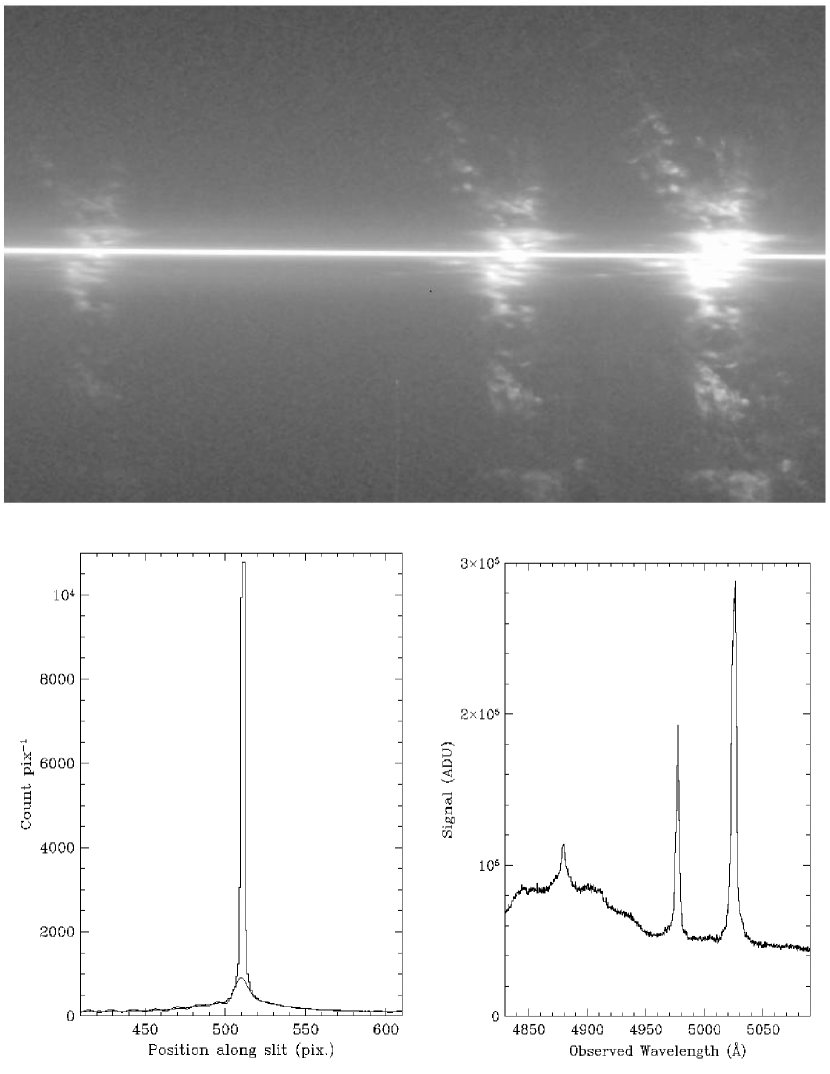
Figure 2: A STIS G430M grating longslit CCD spectrum of the Seyfert I galaxy NGC 4151 covering the emission lines H$\beta$ and [O III] 4959 and 5007Å is shown. Restoration with the inhomogeneous code (background smoothing kernel $\sigma$=4.0 pixels) was performed; and 91 iterations converged to limits of 10^-3 and 2$\times$10^-3 for the point source and background respectively. The PSF spectrum was generated from five TinyTim (Krist, 1995) PSF’s over the wavelength range. The spatial profile at a wavelength of 4930Å (i.e. remote from the emission lines) is shown at lower left (histogram) and the restored spatial profile as a continuous line. Note the extended region of continuum emission which is distinct from the PSF. The spectrum of the extracted point spread function (nuclear broad line region) is shown at lower right; the narrow H$\beta$ and the [O III] lines have very similar width.

5.2 Separating extended line emission from a damped QSO line trough

An important class of astronomical problems involve detecting the spectra of faint extensions around bright point sources, such as the underlying galaxy of a QSO, the optical jet emission from a Pre-Main Sequence star or an AGN. Such cases mandate the careful subtraction of the point source spectrum to reveal the extended spectral features near the point source. Both techniques presented here are well suited to such problems and present a systematic alternative to the ad-hoc approach of PSF fitting (e.g. Moller (2000)). Figure 3 shows an example of a long-slit spectrum across a broad-absorption line QSO (Q2059-360). This is a raw spectrum with sky lines included; the broad Ly-$\alpha$ absorption line is well seen with a trace of extended emission towards its long wavelength edge. The upper, extended object, spectrum is of another galaxy. The data was kindly provided by B. Leibundgut and was taken with the ESO NTT and EMMI spectrometer. There was no suitable bright star nearby to provide the SSF and the spectrum of a spectrophotometric standard with the same set-up had different seeing. The spectrum of the BAL QSO itself was used, with the Ly$\alpha$ region interpolated and smoothed in the dispersion direction. The inhomogeneous technique was employed to separate the Ly$\alpha$ emission source from the BAL continuum spectrum. The right hand panel of Fig.3 shows the result: the bright BAL QSO continuum is very effectively subtracted. The homogeneous technique could also have been used to model the sky background, which when subtracted from the spectrum in Fig.3 reveals the extended Ly$\alpha$ emission source.

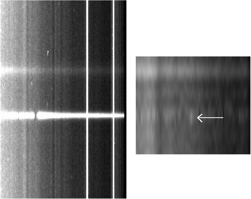
Figure 3: A longslit spectrum across the BAL QSO Q2059-360, including sky background, is shown in the left hand image. Weak extended emission to the right (long wavelength) side of the Ly$\alpha$ trough can be discerned. The right hand panel shows the result of application of the inhomogeneous code with the QSO point source removed and the background remaining. The spatially extended emission of the Ly$\alpha$ emission is arrowed. The smoothing kernel had a $\sigma$=5.0 pixels and 215 iterations were required to reach convergence of 0.0003 for point source and background.

5.3 Extracting many stellar spectra in a globular cluster

The last example is a long-slit spectrum of a globular cluster, in this case NGC 5272 taken with the STIS spectrometer and G430L grating (PI M. Shara, HST proposal 8226). Figure 4 shows how crowded the spectrum is and that there is essentially no region which can be used to estimate the background. About 120 point source spectra could be discerned by eye in this 2D spectrum. Clearly it would be very difficult, if not impossible, to extract the spectra of all the stars on the slit without resort to profile fitting. The positions of all the stars were determined by fitting Gaussians or simple centroids and a PSF was provided by the brightest star in the spectrum, suitably cleaned of its neighbouring spectra. The background is assumed to be composed of sky, very faint cluster members from orbit mixing and bright sources close to the slit edge. Assuming this background does not change its spectral signature across the slit, then the homogeneous technique should be applied. The right hand diagram of Fig.4 shows the spatial profile along the slit and the restored profile of the background with the stars removed. The first attempts showed point source spectra remaining in the background from stars that were closely blended and that were missed in the visual identification. Finally the positions of 129 stars were used as input to the task and their stellar spectra were recovered. Some high excursions in the background remain which suggest the presence of stars omitted from the input catalogue of point sources.

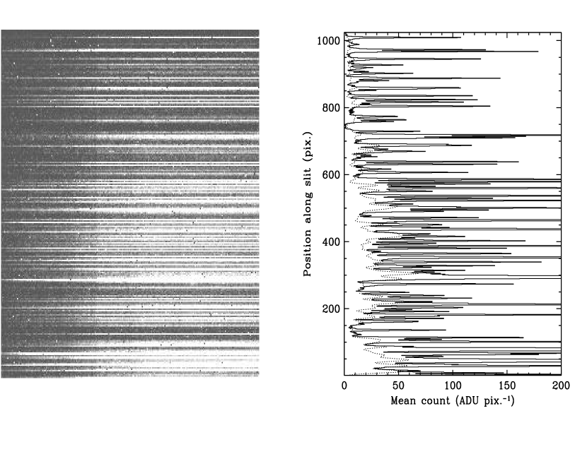
Figure 4: The left hand figure shows a STIS G430L spectrum of the globular cluster NGC 5272 as an example of a very crowded long-slit spectrum (wavelength increasing to the right). 129 point source spectra were fitted in this spectrum using the homogeneous background technique (Sect. 3). The right-hand panel shows the spatial profile of the observed 2D spectrum (bold line) and the restored background with the stars removed (dashed line) after 50 iterations to convergence of 10^-2 for point sources (i.e. maximum difference for all point source fluxes between successive iterations) and 4$\times$10^-3 for background. Note the peaks in the background (e.g. around channel 300) indicative of further point source spectra which were not contained in the input list of sources to extract.

6 Comparison with other techniques

A variety of other methods for separating the spectra of point sources from the spectrum of an extended source have recently appeared. Courbin et al (2000) use an adaption of the MCS image deconvolution algorithm (Magain et al, 1998). The required PSF for the deconvolved image is chosen, and the PSF, which should be applied to restore the data to this chosen PSF, is applied in the deconvolution. In the long-slit case each spectral element is deconvolved independently and three functions are minimized for the fit of the point sources, the smoothness (on the length scale of the output resolution) of the background and the length scale of the correlation in the spectral direction (viz. spectral resolution). The $\chi^{2}$ minimization requires the assignment of two Lagrange multipliers. Since the position of the point-sources is not fitted in the two techniques presented here, only one user-specified parameter - the width of the smoothing kernel for the extended object spectrum - is required in comparison.

Direct PSF fitting has also been applied to the separation of point and extended sources from the spatial component of long-slit spectra. Hynes (2002) presented a method based on the optimal extraction technique to extract spatially blended spectra, but prior subtraction of the extended sources is assumed and not explicitly treated. The maximum entropy method has been used by Khmil & Surdej (2002) in application to overlapping spectra but here separate $\chi^{2}$ minimization cycles are required for the spectra of the point sources, the position of the point sources and the determination of the SSF. Again spatially varying extended sources are not covered by the extraction technique. The two R-L based methods presented here treat the extended source explicitly as part of the restoration process and thus offer a wider range of astrophysical applicability. Both these techniques are based on a well-known image restoration technique.

For unblended spectra of point sources, results obtained with the techniques described here can be compared with those for the optimal extraction method of Horne (1986). As expected - see Sect. 3.4e, the results are then similar, in particular with regard to achieved signal-to noise.

7 Software

The homogeneous and inhomogeneous background extraction codes are included in the STECF IRAF layered package ‘specres’ to extract spectra from longslit or 2-D spectra with an a priori SSF. The input data are the 2D spectrum and the SSF and a table listing the positions of the point sources. The output products are the extracted spectra of the point sources and the restored background image, either with or without the point sources included. A task is also provided in the package to produce an SSF image from sets of (2-D spatial) PSF’s at different wavelengths, simulating the spatial profile produced by placing a long-slit over a point source. Further information and help pages for the routines are available at: http://www.stecf.org/ jwalsh/specres/ The algorithms have been made flexible, can deal with slightly tilted spectra, spatially subsampled SSF’s, and allow the position of point sources to be refined by cross-correlation. A separate table file is output for each extracted point source. Data quality of the input 2D spectrum is considered in order to neglect bad pixels and, if statistical errors are available, then multiple trials can be performed to determine the error estimates on the restored spectra.

8 Conclusions

Two iterative techniques, based on the Richardson-Lucy algorithm, have been presented for decomposing a long-slit spectrum into its constituent parts, namely into the spectra of the point sources and the spectrum of the background. These techniques are applicable to complex fields where standard extraction routines fail or perform poorly. A variety of tests, with real and simulated data, confirm the ability of these techniques to provide effective reductions for complex fields.

References

- Courbin et al (2000) Courbin, F., Magain, P., Kirkove, M., Sohy, S. 2000, ApJ, 529, 1136
- Frieden & Wells (1978) Frieden, B. R., Wells, D. C. 1978, J. Opt. Soc. Am., 68, 93
- Hook & Lucy (1994a) Hook, R.N., Lucy. L.B., Stockton, A., Ridgway, S. 1994, ST-ECF Newsletter 21, 16
- Hook & Lucy (1994b) Hook, R.N., Lucy. L.B., 1994, in Proc. The Restoration of HST Images and Spectra, (eds. R.J. Hanisch & R.L. White), STScI, 86
- Horne (1986) Horne, K. 1986, PASP, 98, 609
- Hynes (2002) Hynes, R. I., 2002, A&A, 382, 752
- Khmil & Surdej (2002) Khmil, S. V., Surdej, J., 2002, A&A, 387, 347
- Hutchings et al (1999) Hutchings, J. B., Crenshaw, D. M., Danks, A. C., Gull, T. R., Kraemer, S. B., Nelson, C. H., Weistrop, D., Kaiser, M. E., Joseph, C. L., 1998, AJ, 118, 2101
- Krist (1995) Krist, J., 1995, in Astronomical Data Analysis Software and Systems IV, ASP Conference Series, Vol. 77, eds. Shaw, R. A., Payne, H. E., Hayes, J. J. E., p. 349
- Lucy (1974) Lucy, L. B. 1974, AJ, 79, 745
- Lucy (1992) Lucy, L. B. 1992, AJ, 104, 1260
- Lucy (1994) Lucy, L.B. 1994, in Proc. The Restoration of HST Images and Spectra, (eds. R.J. Hanisch & R.L. White), STScI, 79
- Magain et al (1998) Magain, P., Courbin, F., Sohy, S., 1998, ApJ, 494, 472
- Moller (2000) Moller, P., 2000. ESO Messenger, No. 99, 26
- Robertson (1986) Robertson, J. G. 1986, PASP, 98, 122
- Richardson (1972) Richardson, W. H. 1972, Jou. Opt. Soc. Am., 62, 55
- Titterington (1985) Titterington, D. M. 1985, A&A, 144,381
- Walsh (1997) Walsh, J. R. 1997, in The 1997 HST Calibration Workshop (eds. S. Casertano, R. Jedrzejewski, T. Keyes, M. Stevens), 156
- Walsh (2001) Walsh, J. R. 2001, ST-ECF Newsletter, No. 28, 5