The Sloan Digital Sky Survey: The Cosmic Spectrum and Star-Formation History.

Abstract

We present a determination of the ‘Cosmic Optical Spectrum’ of the Universe, i.e. the ensemble emission from galaxies, as determined from the red-selected Sloan Digital Sky Survey main galaxy sample and compare with previous results of the blue-selected 2dF Galaxy Redshift Survey. Broadly we find good agreement in both the spectrum and the derived star-formation histories. If we use a power-law star-formation history model where star-formation rate $\propto(1+z)^{\beta}$ out to $z=1$, then we find that $\beta$ of 2 to 3 is still the most likely model and there is no evidence for current surveys missing large amounts of star formation at high redshift. In particular ‘Fossil Cosmology’ of the local universe gives measures of star-formation history which are consistent with direct observations at high redshift. Using the photometry of SDSS we are able to derive the cosmic spectrum in absolute units (i.e. W Å^-1 Mpc^-3) at 2–5Å resolution and find good agreement with published broad-band luminosity densities. For a Salpeter IMF the best fit stellar mass/light ratio is 3.7–7.5 $\hbox{M${}_{\odot}$}/\hbox{L${}_{\odot}$}$ in the $r$-band (corresponding to $\Omega_{\rm stars}h=0.0025$–0.0055) and from both the stellar emission history and the H$\alpha$ luminosity density independently we find a cosmological star-formation rate of 0.03–0.04 $h$ M_⊙ yr^-1 Mpc^-3 today.

1 Introduction

The comoving star-formation rate (SFR) of the Universe is in decline. Since $z=1$ it has dropped by a factor of 3–15 (Cowie et al., 1999; Lilly et al., 1996). At higher redshifts it may have been constant or declining from $z=1$ to $z=5$ but the evidence is that $z=1$ is a critical point for the universal average SFR (Madau et al., 1996; Steidel et al., 1999).

This is a very dramatic conclusion and worth tackling with a variety of complementary observational techniques. One must of course consider how SFR is measured at different redshifts: for $z>1$ the principal observational probe has been rest-frame ultraviolet emission since it is easily accessible in optical bandpasses. Because the UV derives from young stellar populations ($t<<1$Gyr for $\lambda_{\rm rest}\lesssim 2000$Å) the UV flux produced per galaxy will be proportional to the SFR. There are details to do with the contamination from older populations but for $z>1$ and $\lambda_{\rm rest}\lesssim 2000$Å these are minor (Madau et al., 1998). A very important issue though is dust extinction which can be many magnitudes in the UV and in fact represents the principal uncertainty in whether the SFR drops off again at high redshift (see for example Pettini et al., 1998; Steidel et al., 1999). A comprehensive discussion of UV dust extinction issues is given by Bell (2002). Another important issue is the treatment of cosmological surface-brightness dimming which may result in surveys missing a dramatic increase in SFR at high redshift (Lanzetta et al., 2002).

At lower redshifts, where the rest-frame optical spectrum is accessible, alternative methods of calculating SFRs from line emission can be used. The simplest is H$\alpha$ which traces the number of Lyman continuum photons (Glazebrook et al., 1999; Hopkins et al., 2000). This technique has the advantage of using radiation emitted at red wavelengths and is thus considerably less sensitive to dust extinction compared to the UV. Other lines such as H$\beta$ (Tresse & Maddox, 1998a) and [OII] (Hogg et al., 1998) are used but their relationship to SFR is more complicated. For $z<1.5$ some of these lines are accessible in the optical and near-infrared windows and can be used to measure SFRs. A review is given by Hogg (2002) — the vast majority of the surveys that have been carried out indicate considerable evolution in the SFR for $z<1$ although there is disagreement on the amount of evolution required.

A complementary method has been to probe the far-infrared emission of galaxies ($10\micron<\lambda<300\micron$) where dust-processed UV is re-emitted thermally. At high redshifts this must be followed into the sub-mm radio wavelengths. The emission has been used to constrain SFR at low-redshift (Rowan-Robinson et al., 1997) and at high redshift (Hughes et al., 1998) but this approach suffers from both uncertainty in the dust modeling and a lack of spectroscopic redshifts. The latter issue is addressed by fitting the spectral energy distributions (SED) with a series of templates in order to photometrically estimate the redshifts, however there are huge degeneracies between the photometric redshift estimate and the assumed temperature of the dust SED (Blain et al., 2002).

All these approaches involve estimating a luminosity, either continuum or line, per galaxy and then multiplying by the space density in order to give a luminosity per comoving volume. At this point the scale factor, SFR/luminosity, which is where the main uncertainties arise, allows transformation to SFR per unit volume. The light budget per volume is a useful quantity because it allows the stellar emission history of the Universe to be decoupled, in a sense, from its dynamical history (i.e. changes in the number of counted objects by processes such as galaxy formation and galaxy-galaxy merging). This use of luminosity density is a direct method, in which an observed luminosity density at a given redshift is converted to a SFR density at the same redshift.

An alternative approach is that of fossil cosmology where the past history of the Universe is determined from its current contents. This can be done by examining the resolved stellar populations in the Local Group (Hopkins et al., 2001) or in ensembles of galaxies, for example in early type galaxies (e.g. Bernardi et al. (2002); Eisenstein et al. (2002)). Our approach is to look at the ensemble of all galaxies; the ‘Cosmic Optical Spectrum’ of the local Universe. This represents the luminosity-scaled spectra summed over all galaxies. The cosmic spectrum can be thought of as the total emission from all the objects in a representative volume of the Universe. Objects contribute to the cosmic spectrum according to their luminosity. As in the case for an individual galaxy, this spectrum contains a luminosity-weighted mix of features from both old and young stars and we can fit models of star-formation history to it. In particular because the cosmic spectrum represents an average, it will represent the end point of the average SFH. Thus we can fit much simpler models to the cosmic spectrum than are required for the spectra of individual galaxies, since we expect the SFH history of the Universe, as a whole. to vary smoothly with time.

This ensemble approach was applied by Baldry et al. (2002, hereafter BG02) to the cosmic spectrum (meaning the optical spectrum per unit volume) of 166 000 galaxies in the 2dF Galaxy Redshift Survey (2dFGRS, Colless et al., 2001) and derived constraints on allowable star-formation histories (SFH) which agreed well with results derived from direct high redshift measurements via luminosity densities.

The Sloan Digital Sky Survey (SDSS, York et al., 2000) provides many advantages over the 2dFGRS for this type of analysis: it is of higher spectral resolution (though we are not yet able to exploit this in this paper) and will be about four times larger upon completion. The spectral wavelength coverage is larger ($3600\rm\AA<\lambda<8000\AA$ for 2dFGRS and $3800\rm\AA<\lambda<9200\AA$ for SDSS). The photometric calibration is much better as each SDSS multi-fiber observation contains numerous standard stars and can be individually calibrated, whereas for the 2dFGRS a mean calibration was applied to all the survey spectra. The excellent spectrophotometry is borne out by the good agreement between synthetic colors computed from the spectra and actual colors which agree, in average spectra to $<\pm 5$% (Tremonti 2002, private communication). Also the accurate five-color photometry allows comparisons of photometric constraints with color constraints. In particular SDSS is selected in the $r$ band ($\lambda=6200\pm 600$Å), whereas 2dFGRS is selected in $b_{\rm J}$ ($\lambda=4600\pm 700$Å). Thus one would expect SDSS to be more biased toward old massive galaxies and 2dFGRS to be biased toward young, star-forming galaxies. The comparison between the two allows us to investigate the uncertainties in the determination of the SFH.

In this paper we compute the cosmic spectrum for the SDSS local volume, we make a direct comparison with that derived from 2dFGRS by BG02, and we derive new constraints on star-formation history models from the SDSS spectrum. The plan of this paper is as follows. In Section 2 we describe the SDSS data and our methods for combining the spectra to form cosmic spectra. In Section 3 we describe our modeling and fitting procedure and the outcome of the comparison of best fitting SFHs between the SDSS and 2dFGRS surveys. We also test the consistency of models of SFH which form a lot of stars at $z>1$. In Section 4 we generate an absolute cosmic spectrum which we show in physical units. We use this to estimate emission-line luminosity densities and the current SFR density. Finally we give our summary and conclusions (Section 5).

Throughout this paper we take $H_{0}=70\,{\rm km\,s^{-1}\,Mpc^{-1}}$, $\Omega_{m_{0}}=0.3$ and $\Omega_{\Lambda_{0}}=0.7$ for our cosmological quantities, and where appropriate, define $h=H_{0}/100\,{\rm km\,s^{-1}\,Mpc^{-1}}$.

2 Samples used in this analysis

The Sloan Digital Sky Survey is a digital CCD survey in 5 optical bands which intends to cover up to 10 000 deg². An overview is given by York et al. (2000). The imaging camera is described by Gunn et al. (1998), the $ugriz$ photometric system and calibration by Fukugita et al. (1996), Lupton et al. (1999), Hogg et al. (2001) and Smith et al. (2002). A large fraction of SDSS data is currently available to the entire astronomical community (Stoughton et al., 2002). The coordinate system is defined to a precision of better than 0.1 arcsec (Pier et al., 2002). The main galaxy sample is essentially a magnitude limited spectroscopic sample. It is selected as virtually all galaxies in the photometric area with a Petrosian magnitude $r<17.77$. The overall targeting completeness is 92% (Blanton et al., 2002a). For galaxies in this magnitude range the Petrosian magnitude is close to total, they are also close to ‘model magnitudes’ (which are obtained by profile fitting) which represent an alternative method of trying to estimate total magnitudes. Ninety-eight percent of the galaxies span a redshift range of $0<z<0.25$ with a median redshift of 0.10. Full details of the spectroscopic main galaxy sample are given by Strauss et al. (2002). The sample we consider in this paper uses a total of 153 000 galaxies selected to $r<17.70$ (magnitudes are from the PHOTO v5.2 software corrected for Milky Way reddening; see Stoughton et al. (2002) for details) from the SDSS spectroscopic data. The sample is data from 463 survey quality plates in the North Galactic Cap which were observed between MJD 51433 and 5235 and 86 000 galaxies lie in the range $0.01<z<0.11$, the principal range considered in this paper. Only galaxies with secure redshifts were selected.

The spectra are taken through 3.0-arcsec diameter fibers and have a wavelength range of 3800-9200Å and a spectral resolution $\lambda/\Delta\lambda=1800$ which is approximately constant across the spectrum. The signal-to-noise ratio is $>4$ per pixel (pixels width $\simeq$ 1–2 Å). We use ‘smear’ corrected spectra reduced using SPECTRO2D software v4.9. The smear procedure uses dithered telescope pointings to make a low-order correction to allow for aperture effects, it changes the large scale spectral response at the $<\pm 2$% level in the mean colors.

Following BG02, the spectra are combined in redshift slices (using the redshifts from the Princeton 1D spectra pipeline, Schlegel et al. (2003)) by scaling them to their $r$ luminosity and summing them. This scaling provides for a first-order aperture correction. Thus in each slice we get a total luminosity spectrum for all galaxies down to the luminosity limit of the survey at that redshift. Because of the good spectrophotometry of SDSS it is not necessary to apply a correction as was done by BG02.

There are two important issues in using the cosmic spectrum to constrain star-formation histories, the first is luminosity bias and the second is aperture bias. These redshift surveys represent the spectra of all galaxies down to a fixed apparent magnitude. For low redshift galaxies the magnitude limit will correspond to a faint luminosity. Since luminosity densities from typical galaxy luminosity functions (approximately Schechter (1976) functions) tend to converge for $M>M_{*}$, where $M_{*}$ is the Schechter ‘break’ absolute magnitude; once we have sampled more than 2–3 mags below $M_{*}$ the observed cosmic spectrum would be very close to the total spectrum. To be quantitative, for a faint-end slope in the range $-1.3<\alpha<-1.0$ (Blanton et al., 2001; Cole et al., 2001; Cross & Driver, 2002; Madgwick et al., 2002), integrating down to $M_{*}+3$ shows that between 84–94% of the light has been sampled. Thus we expect samples to be highly complete in luminosity at low redshift and give a similar result whether they are selected in $r$ or $b_{\rm J}$.

Figure 1: Comparison of the selection functions of the two surveys. The SDSS $r$ selection filter (solid lines, Stoughton et al.) and 2dFGRS $b_{\rm J}$ selection filter (dashed lines, Hewett & Warren private communication, these include atmosphere and telescope) are shown at redshifts 0.0 and 0.2 (bracketing the redshift range used in this paper). At high redshifts, the $b_{\rm J}$ filter penetrates below the 4000Å break and is therefore more sensitive to younger stellar populations. The dotted line is a theoretical cosmic spectrum from our analysis. The $b_{J}$ curve was converted to photon-response equivalent for comparison with the $r$ curve.

At high redshift we expect the blue/red sample selection to become most prominent in the luminosity bias. In particular for the redshift range we consider the SDSS red selection does not sample below the 4000Å break (Figure 1) where the UV from young stellar populations dominates. Thus we would expect the relative bias to run in favor of older SFHs in the SDSS sample as we approach $z\sim 0.1$ slices.

In contrast, at low redshift we expect aperture effects to be most apparent since the fixed size in arcseconds of the spectroscopic fiber aperture corresponds to smaller physical scales in the galaxy. At high redshift the effects are reversed — the fiber apertures ought to sample most of the light of a galaxy, but we are only seeing the most luminous galaxies and red versus blue selection becomes more important. These sample biases are quantified in Figure 2 which compares the two surveys.

Figure 2: Comparison of sample bias in the SDSS and 2dFGRS redshift surveys. Left: Luminosity bias versus redshift. This shows the fraction of total light of the galaxy population sampled down to the survey magnitude limit, calculated by integrating the appropriate Schechter luminosity function for each survey (Blanton et al., 2001; Madgwick et al., 2002, both are consistent with a faint-end slope of $-1.2$). Right: Projected aperture size versus redshift.

The SDSS data gives us an opportunity to test for aperture bias in a way which was not possible for the 2dFGRS work: because of the excellent SDSS imaging and photometry we can use galaxy colors as a function of aperture size as a diagnostic of aperture bias.

For comparison between the two samples at a common redshift, we define the redshift limits so that the surveys penetrate to the same relative depth below $M_{*}$. For example in the low redshift volume we use $0.02\lesssim z\lesssim 0.05$ for SDSS and $0.03\lesssim z\lesssim 0.06$ for 2dFGRS, the redshift upper limit corresponding to $M_{*}+2.6$ in both cases. The 2dFGRS cosmic spectra are taken from those published by BG02. In Table 1 we define low, medium and high redshift ranges (A, B and C) for which SDSS and 2dFGRS are approximately equivalent in luminosity range. Because the 2dFGRS sample is slightly deeper than the SDSS sample, this correction also works in the direction of minimizing the physical aperture difference, since SDSS fibers are bigger (in arcseconds) than 2dFGRS fibers. This procedure reduces the difference in physical aperture diameter in ranges A,B,C from $\sim$50% to $\sim$25%.

Table 1: Luminosity-bias equivalent redshift ranges (low/medium/high) between the SDSS & 2dFGRS samples

.

Region	2dFGRS redshift range	SDSS redshift range	limiting magnitudesa
A	$0.025<z\leq 0.06$	$0.015<z\leq 0.05$	$M_{*}+4.5$ to $+2.6$
B	$0.06~{}\,<z\leq 0.10$	$0.05~{}\,<z\leq 0.08$	$M_{*}+2.6$ to $+1.4$
C	$0.10~{}\,<z\leq 0.13$	$0.08~{}\,<z\leq 0.11$	$M_{*}+1.4$ to $+0.7$

^a Approximate range of limiting absolute magnitudes from the low-redshift cut to the high redshift cut relative to the Schechter-break luminosity

.

Figure 3: Comparison of SDSS and 2dFGRS cosmic spectra. Three spectra are shown for regions A, B and C as defined in Table 1. The lower set (thin lines) are for SDSS and the upper set (thick lines) are for 2dFGRS (spectro-photometrically corrected). All are normalized by setting the mean flux between 4200 and 5800Å to unity but are offset by multiples of 0.2 for clarity. Note the resolution of SDSS is two to three times better than 2dFGRS.

Figure 3 shows a comparison between the normalized cosmic spectra for SDSS and 2dFGRS for the volumes A,B,C. The 2dFGRS cosmic spectrum has been spectrophotometrically corrected against the model fits as described by BG02. The SDSS spectrum uses the native spectrophotometry. Despite the differences in sample selection and spectral resolution the cosmic spectra look very similar, especially in the absorption features which we use to constrain the SFH. To be quantitative, in region A where we expect the selection bias to be smallest, the RMS of the ratio of the two spectra over the wavelength range 4000Å–8000Å is 2.6% (comparable to the uncertainties in the spectrophotometric modeling quoted by BG02), after smoothing the SDSS spectrum to 2dFGRS resolution. We can break this down into low-pass (i.e. continuum) and high-pass (line) variations using a 200Å smoothing filter. For the smoothed spectra the RMS ratio is 2.4% whereas in the spectra with the smooth component divided out the RMS ratio is only 0.7%. They key point is the high-pass stellar absorption line information is almost identical in the two spectra. The similarity of the cosmic spectra from the two surveys indicate the selection difference is minimal at low redshift. Comparing with the uncertainties quoted by BG02 (which are mostly systematic) we would expect our SFHs from SDSS to agree at the 95% confidence level with those of BG02. It is this detailed modeling of the SFH, to which we now turn.

3 Star Formation Histories derived from cosmic spectra

3.1 Methods

For our modeling of star-formation history we use the empirical ‘double power-law’ parameterization used by BG02. The star-formation rate (SFR) is a simple function of redshift with a break at redshift unity:

$${\rm SFR}\propto\begin{array}[]{cl }(1+z)^{\beta}&\hbox{ for }z<1\\ (1+z)^{\alpha}&\hbox{ for }1\leq z<5\\ 0&\hbox{ for }z\geq 5\\ \end{array}$$

The two power-laws are normalized at $z=1$ and star-formation is started at $z=5$. This simple fitting form is chosen because it already provides a good match to the range of observations of cosmic SFH (for example, see figure 9 of Steidel et al. 1999), has a small number of parameters and provides acceptable fits. Other parameterizations are possible, see BG02 for some examples. All are principally measuring the ratio of old to young stars weighted in some fashion.

The fitting of star-formation histories to the cosmic spectra proceeds using standard evolutionary synthesis techniques and follows that of BG02 for the 2dFGRS data. We use the PEGASE.2 evolutionary synthesis models (Fioc & Rocca-Volmerange, 1997). We assume a universal Initial Mass Function (IMF) which is independent of cosmic epoch and for this we use the IMF of Salpeter (1955). Evolutionary tracks are from the ‘Padova group’ (Bressan et al., 1993) and the stellar atlas comes principally from the theoretical stellar spectra of R. L. Kurucz as given by Lejeune et al. (1997). Metallicity evolution in this code follows the prescription of Woosley & Weaver (1995). The fiducial extinction was chosen as that for a inclination-averaged disk geometry but this makes little difference because, as we will see below, our analysis primarily uses the high-pass spectral information and we varied the extinction to test the effect on the broadband color information.

We use an approach of consistent chemical evolution where the interstellar medium for forming new stars is continuously enriched by the death of old stars. Using the PEGASE.2 closed box model, we control this by a SFR normalization $r$ defined by BG02. This ranges from: $r\sim 0.3$ where only a fraction of the available gas is used to form stars so that the metallicity remains low, to; $r\sim 1.4$ where a total mass of stars is formed over time greater than the mass of gas initially available so that chemical evolution is significantly faster. The metallicity monotonically increases with time and different values of $r$ correspond approximately to different end-point metallicities. We quote end-point metallicity values from PEGASE.2 which are luminosity weighted. We implicitly assume that the range of metallicities at each galaxy epoch can be represented by an average metallicity for the purposes of evolutionary synthesis. This approach is more complicated than using simple-stellar populations (constant metallicity) but is consistent with the logical assumption that older stellar populations should, on average, have a lower metallicity than younger populations.

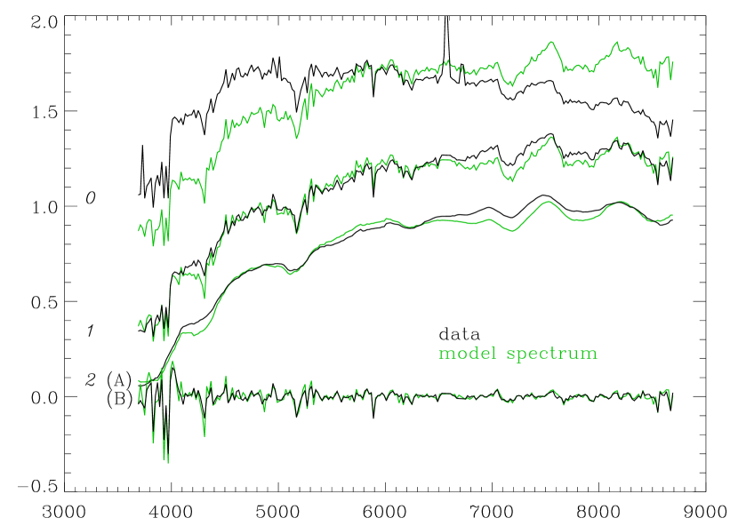
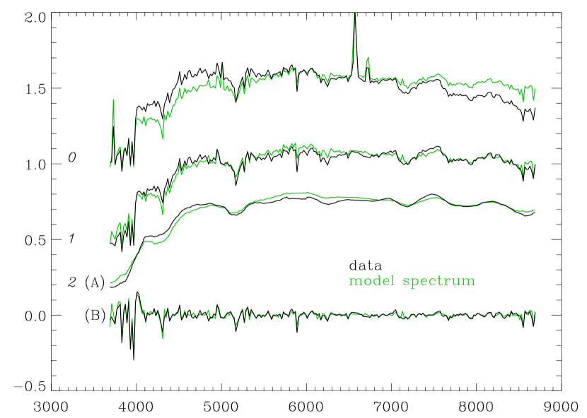
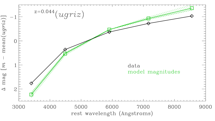
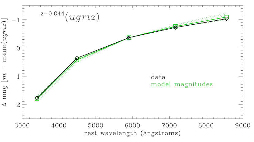
Figure 4: Determination of figures of merit (FOMs). (left column is a poor fit model, right column is a good fit model). Upper: spectral FOMs. The normalized data and and example model spectrum (step 0, offset by $+0.5$) are adjusted by a low-order polynomial to remove power on broad-band scales and some emission lines are cut out to remove nebular components. This forms an adjusted set of spectra (step 1). To compare these, the spectra are further divided into low-pass and high-pass components (step 2 A and B, offset by $-0.3$ and $-1.0$). The FOMs are determined from the $\chi^{2}$ difference between the model and data for each component. Lower: photometric FOM. The broad-band fluxes are coadded without $k$-corrections to form the data ${}^{z}(ugriz)$ magnitudes where $z$ is the mean redshift of the slice. The model magnitudes are calculated by integrating the model spectrum through the redshifted bandpasses. Both are normalized by subtracting the mean of $ugriz$. The FOM is formed from the minimum $\chi^{2}$ difference after comparing the data with 10 different extinction versions of the model magnitudes (dotted lines). The squares represent the fiducial extinction model.

One approach to fitting observed spectra to models would be to compute line indices for both data and models (e.g. Kauffman et al. (2002)). The approach we use here is to fit the entire spectrum using a $\chi^{2}$ statistic. For establishing our goodness of fit, we follow BG02 and compute different $\chi^{2}$ figure of merits (FOMs) from high-pass and low-pass filtered data. As in BG02 we calculate the figure-of-merit quantities by summing over all wavelengths except near strong nebular emission lines (OII 3727Å; OIII 5007Å; H$\alpha$ 6563Å; NII 6583Å; SII 6716Å & 6730Å) as we are only interested in the stellar emission. The first step is to fit the spectrum with a 2^nd order polynomial and divide the spectrum by this fit. This effectively removes power on broad-band scales (i.e. $\sim$ 2000Å resolution). The spectra are then convolved with a 200Å top-hat filter to make a smoothed version and are then divided by this smoothed version. Thus only high-pass spectral information is retained. The $\chi^{2}$ is then the fit between the high-pass model and the high-pass data, using a suitable noise model. This is ‘FOM B’ in the nomenclature of BG02. Another $\chi^{2}$ is computed from the low-pass 200Å resolution spectra (FOM A). Finally we also compute a $\chi^{2}$ fit between SDSS $ugriz$ colors and PEGASE model colors which is illustrated in the lower panel of Figure 4. This final FOM is marginalized over a range of extinction corresponding to about $A_{V}=0.5$–2 mags because of the extinction dependency of this FOM. The upper panel of Figure 4 illustrates the steps in this procedure for data and example model spectra (both bad fits and good fits).

In general, we use only the high-pass FOM or a weighted combination of the FOMs with less weight being given to the low-pass spectral / broadband color information. Examples of residuals for the high-pass FOM are shown in Figure 5. The advantage of this approach is that low-pass systematic uncertainties such as flux calibration errors and dust extinction are effectively excluded. The disadvantage is that broadband color information is also mostly excluded from the analysis. In practice we find this makes little difference since most of the information in the colors is already encoded in the spectral breaks and line indices. Additionly, we note that regions near strong emission lines are excluded from the analysis as we are interested in star-formation history, not the instantaneous SFR that the emission lines are most sensitive to.

Figure 5: Example of residuals from the high-pass analysis: residual squared versus wavelength. The middle panel represents a good-fitting model while the outliers show models rejected at very high formal confidence ($>99.99$%) in comparison with the spectrum from SDSS region A.

To estimate the errors, we follow the approach of BG02 and divide the sample up into 10 contiguous sky areas. We then use the variance between cosmic spectra from different sky areas to estimate the errors, this has the advantage of including systematic effects. Simply taking the raw variance will overestimate the true errors, whilst dividing it by 10 will not properly take into account systematic effects. As a compromise, we estimate the confidence limits with Monte Carlo simulations each time drawing 5 random entries from the 10 regions. This will in principle still overestimate the errors by $\sqrt{2}$ but is robust against systematic effects. In addition, we add $\sim 2$% random errors to the models (with power on all scales from high-pass spectra to broad-band photometry).

3.2 Results

BG02 found the 2dFGRS cosmic spectra exhibited no unique solution but there was a broad curved degeneracy surface in the $\alpha-\beta$ plane. However it did allow the defining of a common solution where all the different measurements of $\alpha-\beta$ agreed. As discussed by Hogg (2002) the surveys to $z=1$ favor $\beta\simeq 3$. Direct UV observations of high redshift galaxies give $\alpha\simeq-1$ (Madau et al., 1996), i.e. a rapid decline, but once these are extinction corrected for dust, estimates range from constant SFR with $\alpha=0$ (Madau et al., 1996; Steidel et al., 1999) to increasing star formation, with $\alpha=1$ for $1<z<1.5$ (Cowie et al., 1999). The problem of the effect of dust extinction, and the sample bias effects such as luminosity and surface brightness selection, is that increasing amounts of UV are missed as one goes to higher redshifts. It has recently been claimed that very large amounts of UV and hence star formation are missed at high redshifts (Lanzetta et al., 2002). So the values of $\alpha$ are really lower limits. This is where the cosmic spectrum constraints become the most useful: only a narrow range is allowed and high $\alpha-\beta$ is excluded. The conclusion of BG02 was that there was a concordance SFH of $1.8<\beta<2.9$ and $-1.0<\alpha<0.7$ that agreed with the various determinations at the 95% level.

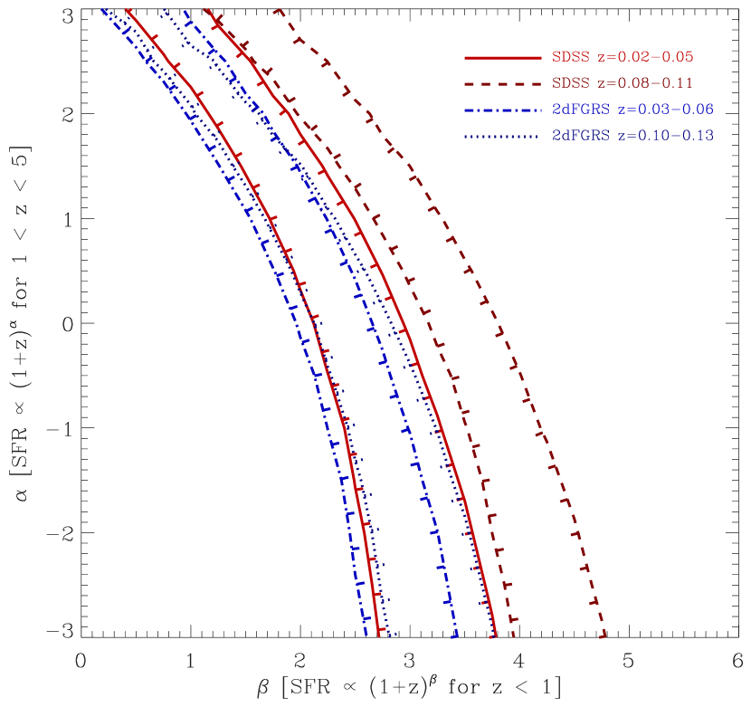
Figure 6: Comparison of star-formation histories derived from the SDSS and 2dFGRS samples in the $\alpha-\beta$ plane for cosmic spectra from redshift regions A and C. The contours represent 90% confidence in our analysis using only the normalized high-pass spectra. For a given $\alpha=0$, the difference between the SDSS and 2dFGRS results amounts to $\Delta\beta\sim 0.25$ for the low-redshift samples and $\Delta\beta\sim 1$ for the high redshift samples.

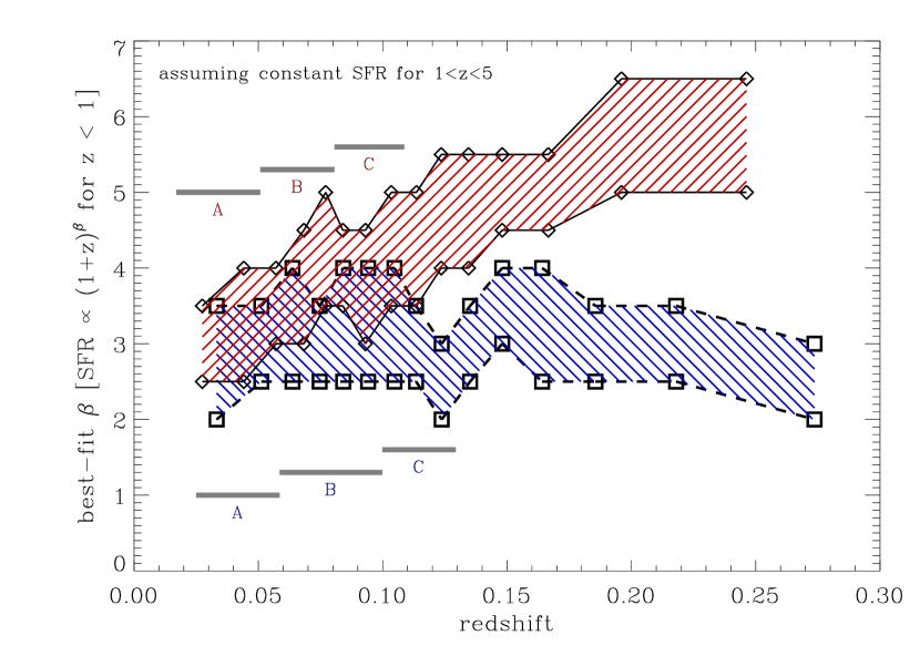
Figure 7: Comparison of star-formation histories derived from different redshift slices. For each slice we plot the 95% confidence region on $\beta$, for $\alpha=0$. The upper region represents the SDSS contours (solid bounding lines) and the lower region represents the 2dFGRS contours (dashed bounding lines). The variation in this plot does NOT represent any cosmic evolution, rather it shows primarily the effect of luminosity-selection bias in measuring cosmic SFH (represented by $\beta$). The divergence is due to the red versus blue selection in the samples as one goes out to high redshift. At low redshift where most of the cosmic light is being counted by both surveys the values of recovered $\beta$ converge. The A,B,C lines show the redshift ranges defined in Table 1. Note that the results here differ slightly from Fig. 6 because here we have marginalized over metallicity in the range 0.5-1.5 Z_⊙.

We compare SDSS and 2dFGRS derived cosmic SFHs by plotting both of them in the $\alpha-\beta$ plane (with $r=1.1$). This is shown in Figure 6 for the two redshift ranges A and C. Contours are shown at the 90% confidence level with only the high-pass FOM applied. In all cases the general shapes of the allowed, degenerate regions are similar, indicating qualitative agreement between the kind of SFHs permitted by SDSS and 2dFGRS cosmic spectra. At low redshift (region A), where we expect the samples to have the least luminosity bias, the agreement is good and well within the formal 90% confidence limits. The difference amounts to $\Delta\beta\simeq 0.25$ for $\alpha=0$ and fixed chemical evolution. This leads to our first important conclusion: the effects of sample selection in the 2dFGRS paper were indeed small at low redshift.

If we look at the higher redshift contours (region C) then there is an obvious shift in the contours from their low-redshift positions, which is the effect of the aforementioned luminosity bias and sample selection. This becomes clearer if we can plot the trend with redshift, to do this in Figure 7 we fix $\alpha=0$ and plot $\beta$ versus redshift for 2dFGRS and SDSS redshift slices. The plot shows 95% confidence regions. Here, we apply a weighted combination of low-pass/broadband and high-pass FOMs but qualitatively the results are the same if only the high-pass information is used. At low redshift, the two regions converge and overlap considerably around $2<\beta<4$ whilst at high redshift the two diverge, which we interpret as the effects of differential luminosity bias in the red versus blue selection. For the red sample the derived $\beta$ for a slice increases considerably approaching $\beta\sim 6$ at $z\sim 0.2$, indicating an increasing dominance of luminous but old red galaxies. In the blue sample this is somewhat counteracted as the blue selection below 4000Å can include more young star-forming galaxies at these redshifts leading to lower values of $\beta\sim 3$ at $z\sim 0.2$. This can be seen directly in the colors: if we match up 2dFGRS redshifts with SDSS photometry we also see much bluer $u-r$ colors for a $z>0.2$ and $b_{\rm J}$$<$19.45 sample (matching the 2dFGRS selection) than for a $z>0.2$ and $r<17.7$ SDSS selection. The effect is strongest for $z>0.2$ where the $b_{\rm J}$ band is pulled below the 4000Å break. We note that at low-redshift the $u-r$ distribution is bimodal with a red-type and blue-type branch (Baldry et al., 2003) whereas at $z>0.2$ the blue peak is gone in the $r$ selected SDSS sample but is still there in the $b_{\rm J}$ selected 2dFGRS sample. The effect of producing a more constant $\beta$ is somewhat fortuitous. One can try making a blue-selected subset of the SDSS spectra, however to be complete for all galaxy types it has to be much brighter (approximately $b_{\rm J}$$<$18.1) and the redshift distribution is too low to show significant effects (98% of galaxies have $z<0.15$ with a median redshift of 0.07). However the important point is that for the lowest redshift slices shown here we have a good approximation to a complete volume limited sample and that the selection function becomes small. For $\alpha=0$ we find from the joint overlap of $2.5<\beta<3.5$ (region A, 95% confidence). If $\alpha$ is increased then $\beta$ comes down.

We have demonstrated by comparison with the completely independent SDSS sample that the effect of luminosity bias, one of the outstanding issues in the 2dFGRS result of BG02, is small. We note the remaining problems of blue versus red samples could be improved, particularly at high redshift, by a multiwavelength selected sample, for example all galaxies jointly in each of $ugriz$ down to a magnitude limit in each band which matched the estimated cosmic spectrum at some redshift.

Figure 8: Plot of $(u-r)_{APER}-(u-r)_{MODEL}$ average colors for a fixed luminosity range in the SDSS sample versus redshift to illustrate aperture effects. (See text for definition of our aperture magnitudes). The $\times$ symbols represent the median, the $+$ symbols the mean and the vertical lines denote the standard deviation (in redshift bins of 0.005). (We plot the latter instead of the standard error on the mean in order to illustrate the scatter). The median and mean values show a small offset at $z<0.05$ but it drops to zero at higher redshift. The dispersion remains large indicating for individual galaxies, as opposed to the mean, aperture effects remain a problem. We also note that the sample is not representative for $z>0.1$ (see text).

The remaining important bias issue to consider is that of aperture effects. The SDSS sample allows us to investigate this for the first time using the colors. In Figure 8 we plot the difference in the average $u-r$ color between ‘model’ SDSS magnitudes and ‘aperture’ SDSS magnitudes which we have computed by integrating the database image profile information to a 3 arcsec diameter aperture. This approximates the SDSS ‘fiber’ magnitudes but has the advantage of being PSF corrected. We choose $u-r$ as it straddles the 4000Å break and should be a color that is very sensitive to changes in stellar populations (Strateva et al., 2001). The 3 arcsec diameter aperture matches the spectroscopic aperture. The model magnitudes are determined by using the best fit of de Vaucouleurs and exponential spatial profiles to calculate a ‘total’ magnitude. We do not use the SDSS Petrosian magnitudes, although these work well for total magnitudes in $griz$ bands we have determined there are significant problems in the use of $u$ Petrosian magnitudes.

It can be seen from Figure 8 that there is no significant difference in the average $u-r$ between model and fiber and no trend with redshift for $z>0.05$. (We note however that at high redshift $z>0.1$ the SDSS becomes dominated by early-type galaxies for which we naturally expect small aperture effects in the colors). For $z<0.05$, there is a small aperture effect amounting to $\Delta(u-r)\lesssim 0.05$ (region A). We stress that for individual galaxies there is a large dispersion in this statistic because aperture bias is a significant problem for individual galaxies. Only in the mean does the aperture bias appear small. Indeed it appears aperture bias from using this low-redshift sample is smaller than the luminosity bias from using higher-redshift samples (region B or C). Given there is no significant aperture effect in the colors, how does this translate into stellar populations? As we know color is degenerate with age and metallicity, so either the stellar populations are the same or there is some fortuitous cancellation in age and metallicity gradients. The latter seems unlikely. The best evidence is that aperture effects are not significant for the cosmic spectrum, i.e. on average. To investigate this in more detail would require two dimensional resolved spectroscopy of a large number of galaxies. We do note that for individual galaxies, for example a face on spiral with a significant old bulge population, aperture effects could be significant. However, there are many types and different orientations of galaxies in a magnitude-limited survey and the average fiber placement on an average galaxy is more robust to aperture effects.

The final value of $\beta$ is still in the range of previous estimates. From SDSS alone: for $\alpha=1$ we constrain $2\lesssim\beta\lesssim 3.5$, and; for $\alpha=0$ we constrain $2.5\lesssim\beta\lesssim 4$. These ranges cover metallicity degeneracy from about solar down to half-solar with approximately 95% confidence limits. The $\beta$ values are close to the 2dFGRS results of BG02. The low-redshift values from the luminosity density measures in UV, nebular lines, far-infrared and radio compiled by Hogg (2002) give a mean $\beta=3.1\pm 0.7$ ($1\sigma$), with a spread in most of the measurements (5 out of 9) of $2.9<\beta<4.5$. The cosmic spectrum and luminosity density measurements are entirely consistent, within their own intrinsic uncertainties, and suggest that $\beta\sim 2$–4.

3.3 Tests of high-redshift star formation

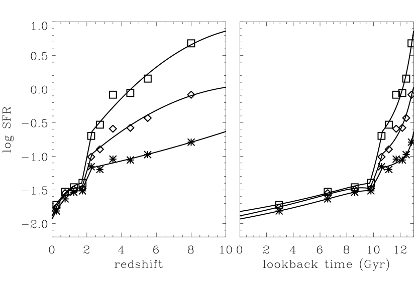
Figure 9: Three possible cosmic SFHs from the analysis of Lanzetta et al. (2002). The symbols represent their data while the solid lines are our fitted to their SFH that we use in our test. The variation is principally at very early times, as illustrated in the right panel. The timescale shown is for the standard $\Lambda$ cosmology with $H_{0}=70$. Note that we only use the average values for each Lanzetta et al. model, i.e. we do not consider their error bars.

As well as the $\alpha-\beta$ parameterization we can test more complex models of SFH. Recently (Lanzetta et al., 2002) proposed that direct high-$z$ surveys were missing a large component of high redshift light based on a comparison with the specific SFR intensity distribution and the column density of Lyman-$\alpha$ absorbers which they claimed were related. This is an ideal situation to test with the cosmic spectrum because even if objects are obscured at high redshift the stars produced must end up in objects in the low-redshift SDSS data, unless of course they form some new local population yet to be detected. We note that Lanzetta et al. proposed these were the ancestors of todays galaxies. They proposed three possible models using different missing-light corrections, from different methods of estimating the SFR intensity distribution function, which we term ‘LOW’, ‘MEDIUM’ and ‘HIGH’ based on their $z>2$ SFRs (Figure 9). All have a low-z slope equivalent to $\beta\approx 1.2$. Note we do not use the $\alpha-\beta$ parameterization, rather we fit the SFHs given by Lanzetta’s figure 4 directly with a break at $z\approx 2$ (see Figure 9 where we replot the Lanzetta figure to illustrate the time dependence and our fit to Lanzetta’s points). The results of fitting these SFHs are given in Table 2. We use a weighted combination of FOM A with FOM B in the ratio of 1-to-5 based on uncertainties determined from the Monte-Carlo error estimation from our different sky regions. For reference we also give the significance levels of a fiducial $\alpha=0$, $\beta=3$ model and a $\alpha=1$, $\beta=2$ model. The first gives a best-fit model with about half-solar metallicity and the second with about solar metallicity.

Table 2: Comparison of SFH models with cosmic spectra

SFH Model	SDSS confidencea	2dFGRS confidencea
$\alpha=0$, $\beta=3$	$<$68.3	68.3
$\alpha=1$, $\beta=2$	80	$<$68.3
Lanzetta LOW	98	68.3
Lanzetta MED	90	90
Lanzetta HIGH	99	99
Lanzetta HIGH $Z>0.5Z_{\odot}$	99.99	99.99

^a Percent rejection for models marginalized over metallicity. The models assume a universal Salpeter IMF and are compared with the low-redshift range cosmic spectra from the surveys. Lanzetta models are integrated for $z<10$.

The HIGH model is rejected at $\geq 99$% confidence for cosmic spectra from both the SDSS and 2dFGRS surveys. In fact, the HIGH model only fits at this level if the average metallicity becomes rather low ($Z<0.5Z_{\odot}$), if we restrict the range to $Z>0.5Z_{\odot}$, the model is rejected very severely. The LOW model is also rejected by the SDSS data because of the low $\beta$, though more marginally. None of these models fit the cosmic spectra as well as our fiducial $\alpha=0$, $\beta=3$ model which is well motivated by the high redshift luminosity density measurements. Thus it appears the cosmic spectrum does not provide any strong evidence for large amounts of missing light in the current high redshift census. Quantitatively, no more than about 85% of stars formed at $z>1$. This is slightly higher than the BG02 upper limit of 80%. The differences are that we include the SDSS data, include only the 2dFGRS low-redshift range, give some weight to the low-pass components of the cosmic spectra and allow $z_{\rm form}=10$ for the Lanzetta models. It is of course possible that some of our assumptions may be wrong, such as a universal IMF; however the data can be well fitted by models which assume a Universal IMF. The slope of the high-mass IMF can be constrained by cosmic spectra, if near-IR data is included. This will be addressed by a forthcoming paper (Baldry & Glazebrook, 2003).

4 The Absolute Cosmic Spectrum

We have shown that we have derived a normalized cosmic spectrum which is consistent between SDSS and 2dFGRS surveys, is close to being volume limited and is robust against aperture effects (by comparing with SDSS $u-r$ colors). An advantage of the SDSS survey is the excellent spectrophotometry as standard stars are included on each plate. In particular we would expect that the relative fluxing with wavelength of the SDSS cosmic spectrum should be much more accurate than for 2dFGRS (BG02 indicate 5–10% errors are likely in the latter). We do indeed find that the SDSS cosmic spectrum is in agreement with the 2dFGRS cosmic spectrum once a good fit spectrophotometric correction has been applied to the latter (see BG02 for details of this procedure, essentially it uses a good fit high-pass model to set the fluxing).

So far we have been dealing with the normalized cosmic spectrum, and principally fitting to the high-pass spectral information. However we can put the cosmic spectrum on an absolute luminosity scale by normalizing to the $r$-band luminosity density. For consistency, we calculate this ourselves from a more recent large-scale structure (LSS) sample by calculating the $r$ luminosity function using $V_{\rm survey}/V_{\rm max}$ weighting and $k$-correcting to the rest-frame $r$-band (kcorrect v1_11, Blanton et al., 2002b). The LSS sample is similar to our cosmic-spectra sample but has a well defined area, includes nearest-neighbor redshifts to replace galaxies missed due to fiber collisions and has stricter limits on the selection magnitude of $14.5<r<17.5$ (taken from sample10 described by Blanton et al., 2002c). A Schechter function fits very well and the total luminosity density is calculated from the analytic total integration (Figure 10). We note there is a small excess of galaxies above the Schechter function fit at low luminosities $M_{r}>-18.5$, a disrepancy that has been noted by other authors (Madgwick et al., 2002) but this has negligible effect on the final luminiosity density (see the lower panel of Figure 10). Regions A and B sample better the faint and bright end of the luminosity function respectively, the luminosity density in these two redshift ranges agrees to $\pm 6$%. For our final $r$ luminosity density we take the value calculated from regions A+B ($0.015<z<0.08$), this is $1.94\pm 0.20\times 10^{8}$ $h$ $L_{\odot}$ Mpc^-3 ($j+2.5\log h=-16.1\pm 0.1$ mags where $j$ is the absolute magnitude of the integrated light per Mpc³). We estimate that the systematic uncertainties (redshift ranges, Schechter fitting) are about 5–10% and quote a 10% error bar. The final value agrees well with the more sophisticated luminosity density calculation of Blanton et al. (2002c).

Figure 10: Luminosity function determined from redshift regions A+B. Upper: The number of galaxies Mpc^-3 mag^-1 versus magnitude with a Schechter function fit (solid line). The vertical bars represent $\pm 3\sigma$ Poisson errors. Lower: A linear scaling of luminosity ($10^{-2.5/{\cal M}}$) versus magnitude, where ${\cal M}$ is the total absolute magnitude Mpc^-3 mag^-1. This shows that the integration of the Schechter function is a good approximation to the luminosity density. This plot uses Petrosian magnitudes but the result is similar if Sersic magnitudes (Blanton et al., 2002c) are used: $j+2.5\log h=-16.11$.

We normalize our cosmic spectrum for region A (where it is the least affected by luminosity bias) to this $r$ luminosity density by integrating the flux of our cosmic spectrum through the $r$-band filter profile (Gunn et al., 1998) and calculating a scaling factor. We note that this will correct to first order for any residual luminosity bias, as the luminosity density is calculated by integrating the Schechter function fit to zero luminosity.

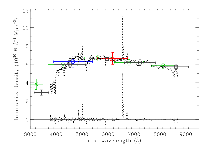
Figure 11: Absolute cosmic spectrum from SDSS region A, i.e. luminosity density per unit wavelength in physical units (dotted line, $h=0.7$). This has been resampled at 10 Angstroms for display clarity. The normalized cosmic spectrum (Fig. 3) was scaled to match the $r$-band luminosity density (Fig. 10) shown by the triangle. The squares show the relative luminosity densities, i.e. flux-weighted observed colors, from region A scaled to the same absolute luminosity density (note they are offset in wavelength to account for the mean redshift of 0.035). The other points represent different estimates of broad-band luminosity densities: asterisks show the redshifted ${}^{0.1}(ugriz)$ filter results of Blanton et al. (2002c) and the diamond shows the $b_{\rm J}$ point of Norberg et al. (2002). The lower spectrum shows the stellar-component-subtracted cosmic spectrum described in the text (shown at the same resolution as above but line luminosities were estimated from the full resolution spectrum as in Fig. 3). This is still in physical units for the line fluxes, i.e. the ordinate units still applies.

This absolute cosmic spectrum (units: Watts Å^-1 Mpc^-3) is shown in Figure 11 (smoothed slightly for the plot) and tabulated in Tables A1 and A2. We can check the reliability of this by comparing the spectrum with luminosity densities computed in other broad bands, these should correspond to smoothed estimates of the cosmic spectrum. In the figure, we overlay the SDSS $ugriz$ luminosity densities from Blanton et al. (2002c), the $b_{\rm J}$ luminosity density from Norberg et al. (2002), and the $ugriz$ luminosity densities calculated by using the cosmic-spectrum sample directly (i.e. combining the photometric $ugriz$ fluxes with the same weighting as the spectra).

There is excellent agreement within the errors. We note that the luminosity densities given by Blanton et al. (2001) are 20–30% discrepant in $u$ and $g$, but the more recent determination shown here from the Blanton et al. (2002c) sample of 150,000 galaxies are in much better agreement with this work, with Cross & Driver (2002), Norberg et al. (2002) and the revised SDSS work of Yasuda et al. (2001). We note some minor differences in analysis: Blanton et al. uses a maximum likelihood method which allows for evolutionary effects (in a set of magnitude-limited samples in each band separately) whereas the Cross & Driver analysis used the $1/V_{max}$ method, and the redshift ranges did not quite match (although both were more or less $0<z<0.15$).

Finally we use our physical cosmic spectrum to derive some interesting quantities. The mass/light ratio of our best-fit models is 3.7–7.5 $\hbox{M${}_{\odot}$}/\hbox{L${}_{\odot}$}$ in the $r$-band (assuming $A_{V}\approx 1$). The range corresponds to the range from a low-metallicity $\alpha=0$ model to the solar metallicity MEDIUM Lanzetta model. Thus from the $r$-band luminosity density we can derive the cosmological mass density in stars: $\Omega_{\rm stars}h=0.0025$–0.0055. Of course this is highly dependent on the assumed Salpeter IMF as the galaxian light is dominated by the most luminous stars. For example the mass-to-light ratio for an IMF with slopes $(-0.5,-1.35)$ broken at 1 M_⊙  is about 60% of the unbroken Salpeter IMF $(-1.35)$. We also computed $\Omega_{\rm stars}h$ for the Kennicutt (1983) IMF $(-0.4,-1.5)$, redoing the fitting, and obtained 0.001–0.002.

Similarly our best fitting range of models also gives us a mean cosmological SFR today, the value range is 0.01–0.04 $h$ M_⊙ yr^-1 Mpc^-3. For a particular choice of $\alpha$ and $\beta$ the range is narrowed as there is only a remaining degeneracy with metallicity. For example if motivated by the high-redshift luminosity density measures we choose $\alpha=0$, $\beta=3$ we find the SFR today is 0.025–0.03 $h$ M_⊙ yr^-1 Mpc^-3. It is also interesting to look at the emission lines in the spectrum, by subtracting the stellar ‘continuum’ and integrating the flux we can derive the local luminosity densities of a whole set of useful lines: [OII], H$\beta$, [OIII], H$\alpha$, [NII] and others. We can do a continuum subtraction by subtracting our best fit SFH stellar model, although the resolution is different the subtraction is still close to zero except near the nebular lines. We used the best fit high-pass model, so as to get the best match to absorption features, and normalize it to the physical cosmic spectrum using a smoothing filter. We show the example continuum subtracted spectrum in Figure 11. The subtraction is excellent in the 4000Å–8000Å region, the principal discrepancy is for wavelengths $>8000$Å where the Calcium triplet absorption lines are not well fit by any of our models; this effect can also be seen in Figure 5.

The line luminosity densities are simply calculated by integrating the cosmic spectrum for each line from $\lambda-8$Å to $\lambda+8$Å. The box width is chosen to be 3$\times$ the typical line FWHM so the fluxes are very close to total.

Table 3: Luminosity density in various lines derived from the cosmic spectrum

Line		Luminosity Density ($10^{30}$ W Mpc-3)
		Region A	Region B
[OII]	3727Å	—	$28\pm 4$
H$\beta$	4861Å	$11\pm 2$	$9\pm 1$
[OIII]	4959Å	$6\pm 2$	$3\pm 2$
[OIII]	5007Å	$22\pm 2$	$13\pm 2$
[OI]	6300Å	$2\pm 1$	$2\pm 1$
[NII]	6548Å	$11\pm 1$	$11\pm 1$
H$\alpha$	6563Å	$70\pm 1$	$59\pm 1$
[NII]	6583Å	$30\pm 1$	$29\pm 1$
[SII]	6716Å	$13\pm 1$	$11\pm 1$
[SII]	6731Å	$10\pm 2$	$8\pm 2$

Notes: (i) Values are quoted for $h=0.7$. Errors on each value are for the continuum subtraction error; (ii) Additional errors of $\pm 10$% should be added to allow for the systematic uncertainty in the $r$ luminosity density.

The resulting line luminosity densities are given in Table 3. We quote values for region A and B, as the latter includes [OII] and for comparative purposes. Both are normalized to the same $r$ luminosity density. There are two sources of error: firstly the imperfection of the continuum subtraction. Visually we checked the region around each line, particularly the Balmer lines, and found no evidence of significant residuals, i.e. the plot appears as an emission line with zero continuum plus ‘noise’ due to the mismatch in resolution between raw data and model spectrum. To quantify this for each line we similarly extract two regions, either side of the line, of the same width where there is only blank continuum, i.e. typically a 40-60Å offset. (These are optimized for each line particularly in the crowded H$\alpha$/[NII] region). These give typically the same error and we quote the maximum in the table. There is also an additional systematic error due to the uncertainty in the $r$ luminosity density which we estimate as 10%.

The line luminosity densities lead to some interesting results: first the Balmer decrement H$\alpha$/H$\beta$ is $6.4\pm 0.9$ (region A but region B is similar), if we take an unreddened case B recombination value of 2.86 (Hummer & Storey, 1987) and a Milky Way dust law from Pei (1992) (the SMC law gives similar numbers as the two are close in the optical) we derive a nebular extinction $A_{V}=2.4\pm 0.4$. The $H\alpha$ luminosity density thus requires a correction factor of $\times(5.8\pm 1.8)$. This is consistent with other workers findings — for example we have re-analyzed the sample of Gallego et al. (1995) looking at the $H\alpha$ correction factor as a function of luminosity and find a volume averaged value of $\times 4.6$. Thus it makes little difference whether one dereddens before taking the mean or simply dereddens the mean (which is the approach we are taking here with the cosmic spectum) even for these large nebular extinction values.

The dereddened $H\alpha$ luminosity density is thus $4.1\pm 1.3\times 10^{32}$ W Mpc^-3 for $h=0.7$. Converting to cgs units and $h=0.5$ this gives $2.9\pm 0.9\times 10^{39}$ ergs s^-1 Mpc^-3 which is the same as that found by from the Canada France Redshift Survey (Tresse & Maddox, 1998b) at low redshift ($z\sim 0.2$). It is twice as high as that found by the objective prism survey of Gallego et al. (1995).

From our models we can also work out the conversion of H$\alpha$ luminosity into SFR (from the number of ionizing photons), the mean conversion factor is $1.36\times 10^{41}$ ergs s^-1 M_⊙^-1 yr and the range in the models is $\pm 15$% (it varies with metallicity). This allows us to derive a SFR density today of $0.030$ – $0.056$ $h$ M_⊙ yr^-1 Mpc^-3. It is remarkable to note that this is entirely consistent with the derived independently from the star-formation history fitting which illustrates the validity of our general approach. The H$\alpha$ line independently measures the instantaneous SFR from young ionizing stars, whereas the SFH fits a model to the stellar continuum and is averaged over several Gyr. It is interesting to note that given the cosmic spectrum to get a SFR from SFH fitting much lower than 0.03 $h$ M_⊙ yr^-1 Mpc^-3 requires high $\beta$, high $\alpha$ AND a low metallicity today.

We note that the Gallego et al. (1995) sample also gives a lower SFR density than the UV sample of Treyer et al. (1998). Both Treyer et al. (1998) and Tresse & Maddox (1998b) are measured at $z\sim 0.2$, whereas the current sample is $z\sim 0.05$ which is comparable to the redshifts of the Gallego et al. (1995) sample. It is only the latter which is discrepant. The most likely explanation is that the Gallego et al. (1995) survey covers only $1/5^{\rm th}$ our sky area and is only sensitive to star-forming galaxies as it is emission line selected. Our survey represents a ‘cosmic average’ and galaxies contribute to the final cosmic spectrum even if the H$\alpha$ flux is not detectable in individual galaxies. We note that H$\alpha$ is only sensitive to transient star-formation over $\sim 20$ Myr whereas a UV sample like those of Treyer et al. (1998) effectively average over longer times scales of up to $\sim$ 1 Gyr (see Glazebrook et al. (1999) for a discussion of this).

A final comment on the other line ratios: the observed H$\alpha/$[OII] line ratio of 2.1 (region B) is entirely consistent with the median found by the sample of galaxies observed by Kennicutt (1992). The other line ratios are also entirely consistent with those from star-forming galaxies (Veilleux & Osterbrock, 1987) including the weak [OI] line, indicating that the AGN contribution to the cosmic spectrum is indeed negligible. It can at most be only a few percent according to the models of Kewley et al. (2001). Most of the optical light of the Universe does indeed come from stellar nucleosynthesis.

5 Summary and Conclusions

Computing the light in the Universe today from the SDSS and 2dFGRS surveys allows us to derive a cosmic optical spectrum, determine its robustness, and make more accurate determinations of allowable star-formation histories of the Universe. In particular:

1. We find a range of solutions $2<\beta<3$ and $0<\alpha<1$ which are consistent with the cosmic spectrum and determinations of the evolution of the luminosity density in various bands.

2. ‘Fossil Cosmology’ and direct cosmology agree: i.e. the SFH inferred from the local Universe agrees with that measured by luminous emission at high redshift. Again the Copernican Principle, that we are in no special place in the universe, is demonstrated by observational astronomy.

3. There is good agreement between SDSS and 2dFGRS derived cosmic spectra and SFHs at low-redshift, where we expect luminosity biases to be minimal, despite the difference in aperture. We conclude the result is robust against luminosity selection effects.

4. The excellent photometry of SDSS allows us to test for aperture effects; for average quantities such as the mean color and hence the cosmic spectrum we find the aperture effects are not significant (though they are still important for individual galaxies).

5. Due to the excellent spectrophotometric quality of the SDSS data we can make an absolutely calibrated cosmic spectrum for a close to volume limited sample.

6. None of the SFH scenarios proposed by Lanzetta et al. (2002) fit the cosmic spectrum as well as more standard models. There appears to be no compelling evidence for missing star-formation at high redshift from the cosmic spectrum.

7. Typically good fits to the cosmic spectrum (using consistent chemical evolution) give a final metallicity of 0.5–1 Z_⊙.

8. We find the stellar population of the universe today has a best fit $r$-band mass/light ratio (for Salpeter IMF) of 3.7–7.5 $\hbox{M${}_{\odot}$}/\hbox{L${}_{\odot}$}$, which given the $r$-band luminosity density of $j+2.5\log h=-16.1$ gives $\Omega_{\rm stars}h=0.0025$–0.0055 (and a factor of 2 lower for a Kennicutt IMF).

9. By fitting the best stellar population model and subtracting, we can derive a whole set of nebular line luminosity densities for our cosmological volume. In particular we find the local dereddened H$\alpha$ luminosity density is twice as high as found by Gallego et al. (1995) and similar to that found by Tresse & Maddox (1998b).

10. We find the SFR of the Universe today (for Salpeter IMF) is 0.03–0.04 $h$ M_⊙ yr^-1 Mpc^-3, and agrees between models fit to the stellar population and that derived from the H$\alpha$ luminosity density of the same sample.

5.1 Future Work

One avenue which it is clearly possible to explore is how the SFH varies with the luminosity of galaxies. The cosmic spectrum represents a binned approach, i.e. looking at the ensemble stellar population in a volume and inferring the SFH. We can not specify which galaxies the stars were in at earlier times, i.e. it is not sensitive to merging. We can extend this approach by computing the cosmic spectrum in luminosity bins, i.e. estimating the SFH of stellar populations as a function, approximately, of the mass of the galaxy they end up in today. Does the SFH depend significantly on this? Given known color-luminosity relationships which extend across a range of Hubble types (e.g. Gavazzi, 1993, figure 4) obviously we expect it too.

In fact we have seen already some evidence for this in the current paper, where the selection effect of the magnitude limit causes the high redshift part of the SDSS survey to have higher luminosities and steeper values of $\beta$. Luminous galaxies on average contain older stellar populations. In the next paper in this series (Baldry et al., 2003) we present a detailed analysis of this differential SFH in today’s Universe.

One limitation of this work is the assumption of a universal Salpeter IMF. The high-mass IMF can be constrained by cosmic spectra, if near-IR data is included. This will be addressed by a forthcoming paper (Baldry et al., 2003).

Another limitation of the current work is the dependence on relatively low resolution (20Å) models of evolutionary synthesis, whereas the SDSS data has 2–5Å resolution. The SDSS cosmic spectrum resolves many low equivalent width metal lines which are not exploited by the current low resolution analysis and will help to break the age-metallicity degeneracy. We are working toward being able to construct high-resolution models to resolve further the question of the star-formation history of the Universe.

Table A1. Cosmic Spectrum for Region A.

Rest Wavelength	Luminosity	Continuum subtracted luminosity
Å	$10^{30}$ W Å-1 Mpc-3	$10^{30}$ W Å-1 Mpc-3
6556.6	6.48919	0.30760
6558.1	7.10810	0.96345
6559.6	9.73218	3.62092
6561.1	15.42100	9.34124
6562.7	19.65739	13.61270
6564.2	16.94022	10.92763
6565.7	10.88128	4.90330
6567.2	7.43149	1.47872
6568.7	6.54169	0.62419
6570.2	6.34205	0.44839

Note: Only a sample 10 rows are shown in a wavelength region near H$\alpha$. The full table covering 3764Å–8697Å is available from the electronic edition.

Table A2. Cosmic Spectrum for Region B.

Rest Wavelength	Luminosity	Continuum subtracted luminosity
Å	$10^{30}$ W Å-1 Mpc-3	$10^{30}$ W Å-1 Mpc-3
3723.7	4.10668	1.17038
3724.6	5.54068	2.62494
3725.4	6.87602	3.97530
3726.3	7.58438	4.70544
3727.2	8.05617	5.19847
3728.0	8.50139	5.66404
3728.9	8.14010	5.32336
3729.7	6.53688	3.74197
3730.6	4.65805	1.85869
3731.4	3.45462	0.63813

Note: Only a sample 10 rows are shown in a wavelength region near [OII]. The full table covering 3636Å–8458Å is available from the electronic edition.

References

- Baldry & Glazebrook (2003) Baldry, I. K. & Glazebrook, K. 2003, ApJ, in preparation
- Baldry et al. (2002) Baldry, I. K. et al. 2002, ApJ, 569, 582 (BG02)
- Baldry et al. (2003) —. 2003, ApJ, in preparation
- Bell (2002) Bell, E. F. 2002, ApJ, 577, 150
- Bernardi et al. (2002) Bernardi, M. et al. 2002, MNRAS, submitted
- Blain et al. (2002) Blain, A. W., Barnard, V. E., & Chapman, S. C. 2002, MNRAS, in press (astro-ph/0209450)
- Blanton et al. (2002a) Blanton, M. R., Lupton, R. H., Maley, F. M., Young, N., & Loveday, J. 2002a, AJ, in press (astro-ph/0105535)
- Blanton et al. (2001) Blanton, M. R. et al. 2001, AJ, 121, 2358
- Blanton et al. (2002b) —. 2002b, AJ, in press (astro-ph/0205243)
- Blanton et al. (2002c) —. 2002c, ApJ, submitted (astro-ph/0210215)
- Bressan et al. (1993) Bressan, A., Fagotto, F., Bertelli, G., & Chiosi, C. 1993, A&AS, 100, 647
- CIE (1986) CIE. 1986, publ. no. S002, Standard on Colorimetric Observers (Commission Internationale de l’Éclairage)
- Cole et al. (2001) Cole, S. et al. 2001, MNRAS, 326, 255
- Colless et al. (2001) Colless, M. et al. 2001, MNRAS, 328, 1039
- Cowie et al. (1999) Cowie, L. L., Songaila, A., & Barger, A. J. 1999, AJ, 118, 603
- Cross & Driver (2002) Cross, N. & Driver, S. P. 2002, MNRAS, 329, 579
- Eisenstein et al. (2002) Eisenstein, D. et al. 2002, ApJ, in press (astro-ph/0212087)
- Fioc & Rocca-Volmerange (1997) Fioc, M. & Rocca-Volmerange, B. 1997, A&A, 326, 950 (PEGASE)
- Fukugita et al. (1996) Fukugita, M., Ichikawa, T., Gunn, J. E., Doi, M., Shimasaku, K., & Schneider, D. P. 1996, AJ, 111, 1748
- Gallego et al. (1995) Gallego, J., Zamorano, J., Aragon-Salamanca, A., & Rego, M. 1995, ApJ, 455, L1
- Gavazzi (1993) Gavazzi, G. 1993, ApJ, 419, 469
- Glazebrook et al. (1999) Glazebrook, K., Blake, C., Economou, F., Lilly, S., & Colless, M. 1999, MNRAS, 306, 843
- Gunn et al. (1998) Gunn, J. E. et al. 1998, AJ, 116, 3040
- Hogg (2002) Hogg, D. W. 2002, PASP, submitted (astro-ph/0105280)
- Hogg et al. (1998) Hogg, D. W., Cohen, J. G., Blandford, R., & Pahre, M. A. 1998, ApJ, 504, 622
- Hogg et al. (2001) Hogg, D. W., Finkbeiner, D. P., Schlegel, D. J., & Gunn, J. E. 2001, AJ, 122, 2129
- Hopkins et al. (2000) Hopkins, A. M., Connolly, A. J., & Szalay, A. S. 2000, AJ, 120, 2843
- Hopkins et al. (2001) Hopkins, A. M., Irwin, M. J., & Connolly, A. J. 2001, ApJ, 558, L31
- Hughes et al. (1998) Hughes, D. H. et al. 1998, Nature, 394, 241
- Hummer & Storey (1987) Hummer, D. G. & Storey, P. J. 1987, MNRAS, 224, 801
- Kauffman et al. (2002) Kauffman, G. et al. 2002, MNRAS, in press (astro-ph/0205070)
- Kennicutt (1983) Kennicutt, R. C. 1983, ApJ, 272, 54
- Kennicutt (1992) —. 1992, ApJ, 388, 310
- Kewley et al. (2001) Kewley, L. J., Dopita, M. A., Sutherland, R. S., Heisler, C. A., & Trevena, J. 2001, ApJ, 556, 121
- Lanzetta et al. (2002) Lanzetta, K. M., Yahata, N., Pascarelle, S., Chen, H., & Fernández-Soto, A. 2002, ApJ, 570, 492
- Lejeune et al. (1997) Lejeune, T., Cuisinier, F., & Buser, R. 1997, A&AS, 125, 229
- Lilly et al. (1996) Lilly, S. J., Le Fevre, O., Hammer, F., & Crampton, D. 1996, ApJ, 460, L1
- Lupton et al. (1999) Lupton, R. H., Gunn, J. E., & Szalay, A. S. 1999, AJ, 118, 1406
- Madau et al. (1996) Madau, P., Ferguson, H. C., Dickinson, M. E., Giavalisco, M., Steidel, C. C., & Fruchter, A. 1996, MNRAS, 283, 1388
- Madau et al. (1998) Madau, P., Pozzetti, L., & Dickinson, M. 1998, ApJ, 498, 106
- Madgwick et al. (2002) Madgwick, D. S. et al. 2002, MNRAS, 333, 133
- Norberg et al. (2002) Norberg, P. et al. 2002, MNRAS, 336, 907
- Pei (1992) Pei, Y. C. 1992, ApJ, 395, 130
- Pettini et al. (1998) Pettini, M., Kellogg, M., Steidel, C. C., Dickinson, M., Adelberger, K. L., & Giavalisco, M. 1998, ApJ, 508, 539
- Pier et al. (2002) Pier, J. R., Munn, J. A., Hindsley, R. B., Hennessy, G. S., Kent, S. M., Lupton, R. H., & Ivezic, Z. 2002, AJ, in press (astro-ph/0211375)
- Rowan-Robinson et al. (1997) Rowan-Robinson, M. et al. 1997, MNRAS, 289, 490
- Salpeter (1955) Salpeter, E. E. 1955, ApJ, 121, 161
- Schechter (1976) Schechter, P. 1976, ApJ, 203, 297
- Schlegel et al. (2003) Schlegel, D. J. et al. 2003, ApJ, in preparation
- Smith et al. (2002) Smith, J. A. et al. 2002, AJ, 123, 2121
- Steidel et al. (1999) Steidel, C. C., Adelberger, K. L., Giavalisco, M., Dickinson, M., & Pettini, M. 1999, ApJ, 519, 1
- Stoughton et al. (2002) Stoughton, C. et al. 2002, AJ, 123, 485
- Strateva et al. (2001) Strateva, I. et al. 2001, AJ, 122, 1861
- Strauss et al. (2002) Strauss, M. A. et al. 2002, AJ, 124, 1810
- Tresse & Maddox (1998a) Tresse, L. & Maddox, S. J. 1998a, ApJ, 495, 691
- Tresse & Maddox (1998b) —. 1998b, ApJ, 495, 691
- Treyer et al. (1998) Treyer, M. A., Ellis, R. S., Milliard, B., Donas, J., & Bridges, T. J. 1998, MNRAS, 300, 303
- Veilleux & Osterbrock (1987) Veilleux, S. & Osterbrock, D. E. 1987, ApJS, 63, 295
- Woosley & Weaver (1995) Woosley, S. E. & Weaver, T. A. 1995, ApJS, 101, 181
- Yasuda et al. (2001) Yasuda, N. et al. 2001, AJ, 122, 1104
- York et al. (2000) York, D. G. et al. 2000, AJ, 120, 1579