Emission Line Galaxies in the STIS Parallel Survey II: Star Formation Density111Based on observations made with the NASA/ESA Hubble Space Telescope, obtained from the data archive at the Space Telescope Science Institute, which is operated by the Association of Universities for Research in Astronomy, Inc., under NASA contract NAS 5-26555.
Abstract
We present the luminosity function of [OII]-emitting galaxies at a median redshift of , as measured in the deep spectroscopic data in the STIS Parallel Survey (SPS). The luminosity function shows strong evolution from the local value, as expected. By using random lines of sight, the SPS measurement complements previous deep single field studies. We calculate the density of inferred star formation at this redshift by converting from [OII] to H line flux as a function of absolute magnitude and find M⊙ yr-1 Mpc-3 at a median redshift within the range ( km s-1 Mpc-1, ). This density is consistent with a evolution in global star formation since . To reconcile the density with similar measurements made by surveys targeting H may require substantial extinction correction.
1 Introduction
The comoving density of global star formation in the Universe has decreased significantly since a redshift of (Hogg 2002; Madau, Pozzetti, & Dickinson 1998; Madau et al. 1996), but the details of the evolution are still uncertain. Extensive measurements of the star-formation history have concentrated on surveys for H emission (e.g. Gallego et al. 1995, Yan et al. 1999, Tresse et al. 2002) and the UV continuum (e.g. Lilly et al. 1996, Connolly et al. 1997). A correction factor is needed reconcile the two methods (Calzetti et al. 1997; Tresse & Maddox 1998; Glazebrook et al. 1999) as dust obscuration is expected to hide some significant fraction of star formation in the distant Universe. Complementary optical data is provided by targeting the [OII] emission line, which can also provide a direct measurement of the rate of star-formation, though its calibration depends on the metallicity and ionization state of the gas, as well as the reddening (Kennicutt 1998). Indeed, surveys at higher redshift will need to depend on the oxygen line. At , the H line redshifts out of the K-band, making it inaccessible to ground-based NIR spectrometers. As a result, [OII] emission is the best rest-frame optical tracer of star-formation available at high redshift until NGST.
In this paper, we present analysis of the deepest spectroscopic fields in the STIS parallel survey (SPS; Gardner et al. 1998). Our motivation is to determine the comoving density of star-formation at as inferred from the [OII] emission line. The deep SPS data cover 141 square arcminutes, and detect objects down to continuum magnitudes of in filterless imaging, with emission line strengths as faint as ergs cm-2 s-1 (Teplitz et al. 2002, hereafter Paper I). These data are complementary to other surveys of the [OII] luminosity density. Hogg et al. (1999a; hereafter H99) measured [OII] emission in 375 galaxies with from the redshift survey data in the 50 square arcminute “Caltech area” (Cohen et al. 2000) around the Hubble Deep Field North (HDF; Williams et al. 1996). The HDF spectra obtained with LRIS (Oke et al. 1995) on the Keck telescopes measure emission lines to a limit 15 times fainter than the SPS. Prior to H99, the best measurement of the [OII] luminosity density was obtained the Canada France Redshift Survey (CFRS; Lilly et al. 1995) by Hammer et al. (1997, hereafter CFRS9). A significant increase in [OII] luminosity is seen with lookback time in the range (Cowie et al. 1996; Gallego et al. 2002).
Throughout the paper, we will adopt a flat, -dominated universe ( km s-1 Mpc-1, ), except where otherwise noted.
2 The Data
The slitless spectroscopic capability of STIS, using the G750L grating with spectral resolution of at 7500Å, allowed a random-field redshift survey for star-forming galaxies at . The deepest 219 of the fields, which were observed by STIS in parallel with targeted HST observations, contain 78 objects identified with [OII] emission (Paper I). Of these, 14 have multiple emission lines, providing secure redshifts. For the rest, the identification of a single line as [OII] is based on the non-detection of other lines, together with photometric information from the paired direct filterless imaging. A signal to noise limit of was imposed for the strongest line in an object in order for it to be included in the catalog. For the present analysis, we impose a redshift cutoff of to avoid the objects in the poor sensitivity region at Å. In total, we include 71 of the 78 [OII]-emitters from Paper I.
The SPS detections are biased towards objects with a strong contrast between line and continuum. This bias means most SPS line-emitters are morphologically compact and that most of the emission lines have high equivalent width (EW). The SPS detection limit is Å for observed EW, consistent with the values for most galaxies undergoing rapid star-formation (Kennicutt 1992). The measured EW value is uncertain for most SPS objects due to low significance of continuum measurement in the spectra. Typically the continua are measured with a signal-to-noise ratio (SNR) of per two-pixel resolution element. The continuum is measured over many resolution elements (typically ), but is still a major source of error in the EW. Figure 1 compares the EW distribution for the SPS with that of other [OII] surveys at similar redshifts. The SPS objects have a median rest-frame EW for [OII] of Å, but many of the Å objects have poor continuum detections, so that the EW may be overestimated (see H99). It appears from the figure that the SPS is missing a substantial portion of low EW lines, particularly at low redshift. At high redshift, low EW lines may simply have been missed in all of the surveys. Nonetheless, CFRS9 and Cowie et al. (1996) both conclude that there is a strong increase in the fraction of galaxies with strong [OII] emission ( Å) at .
2.1 Incompleteness
The SPS survey detects Å in the observational frame. Figure 2 shows the distribution of missing low-EW objects as a function of [OII] luminosity, based on H99. In the analysis of the SPS sample, we correct for this incompleteness. Because the H99 published data only present the equivalent width distribution for objects with continuum detection (), this incompleteness correction is strictly an upper limit.
The primary source of incompleteness in the SPS sample is missing objects that would have met the selection criteria. Visual detection by multiple observers was more accurate than any available automated detection scheme, but human error remains a factor. Simulated spectroscopic images were used to determine the completeness level of our detection scheme. Test images were created by inserting known spectra into SPS frames and trying to recover them. Two spectra were used as the basis of this experiment, one with and the other with . Both spectra were high signal to noise (), but were scaled to lower significance in the test frames. The emission line itself was moved within the spectrum to prevent identification by pattern matching. The spectra were inserted at random spots in randomly chosen images and scaled to an emission line signal-to-noise ratio of 3–7. For each test case, 300 simulated frames were created. In some frames, continuum spectra were also added without an emission line to further disguise the simulated data. Table 1 lists the resulting incompleteness as a function of EW and SNR. The completeness of the survey at any given SNR and EW value is obtained by interpolating between the data points in the table.
3 Calculating the Luminosity Function
We use the method to calculate the luminosity function (LF) of [OII] emission lines. For each galaxy we determine the comoving volume over which it could be detected in our survey. The volume is different for each of the parallel fields, based on the limiting flux. Assuming we have detections in fields, then for a single galaxy in a single field we have, following Hogg (1999b) :
| (1) |
where,
| (2) |
and, is the angular diameter distance, which in the case of a flat, matter dominated universe is:
| (3) |
Further, is a function of z, because the available area depends on the placement of the observed wavelength of the line and the position of the object within the field of view. That is, if the object is too far to one side, the line will fall off the edge of the detector. So for an detector, a central wavelength , a line at rest wavelength and a dispersion ,
| (4) |
The effective area of the detector is slightly smaller than the default field of view (51.2′′′′), since we only consider the region of the registered frame with the full exposure time. Similarly, we do not consider area blocked by very bright stars or local galaxies (see the first table in Paper I).
The volume integral is over to , as defined by the signal-to-noise in the line. In an exposure with limiting flux , a line that is detected at with flux and originating at would be have been observable at any such that
| (5) |
where is the sensitivity function of the spectrum, normalized to unity at , and is the luminosity distance
| (6) |
The individual for the each of the survey fields are summed for each galaxy to obtain its . Finally, the number density of galaxies in a luminosity bin of width is obtained by:
| (7) |
where is the inverse of the completeness function at the SNR and EW of the detected line. Figure 3 shows the SPS [OII] luminosity function compared to that of H99 and the local measurement (Gallego et al. 2002). The SPS measurement appears systematically underdense at high luminosities. Only two objects contribute to the last bin, so missing or misidentified objects may be the cause of that bin being so extreme an outlier. The flattening of the H99 LF at low luminosities compared to the SPS measurement might be expected given the H99 magnitude limit, since H99 do not detect the high-EW galaxies that make up much of the SPS sample and may contribute to the faint end of the LF. The LF inferred from SPS shows strong evolution with respect to the local LF, as expected.
4 Comoving Density of Star-Formation
H emission is a good indicator of star formation because it traces the ionizing flux from hot stars. To infer the star formation rate (SFR) in a galaxy from [OII] emission, it is necessary to assume an [OII]:H ratio. This ratio has an average of 0.45 for local galaxies (Kennicutt 1998), but is highly dependent on the metallicity and reddening of the individual galaxy. Jansen, Franx, & Fabricant (2001) show that the ratio can vary by up to a factor of 7, and that it has a strong inverse correlation with continuum luminosity. We adopt the relation they find for local galaxies with strong H emission (EW(H) Å):
| (8) |
Jansen et al. find considerable scatter about this relation. Apparently, the relation holds at higher redshift (; Tresse et al. 2002), but it has not been tested on many objects, and it may not hold in all cases (Hicks et al. 2002). If we instead use the average value for the ratio of [OII] to H, then we obtain similar results though the distribution of H luminosities has less outliers; that is, we find fewer galaxies with or .
In order to apply the Jansen et al. relation, it is necessary to know the rest-frame of each galaxy. The SPS images are taken with the STIS filterless CCD, which admits a much wider wavelength range than the B filter. We adopt a continuum slope proportional to wavelength, except in cases where a good detection of the continuum in the spectrum allows direct measurement. This conversion is an important systematic error in the SPS data, and in the future could be improved with photometry of the emission line objects in several filters. The average value of [OII]:H remains close to 0.45 for the SPS sample using the Jansen et al. relation, but some individual galaxies change by a factor of more than two.
Figure 4 shows the luminosity function of SPS emission lines converted to H, compared to other measurements of LF(H) at similar redshifts, from the literature. Of particular interest are the comparisons to measurements made with NICMOS slitless spectroscopy on HST (Thompson et al. 1998). The NICMOS parallels (McCarthy et al. 1999; Yan et al. 1999) are a survey comparable in many respects to the SPS, since they are biased towards compact high-EW objects and sensitive to a similar range of luminosities. The NICMOS parallels do not detect lines with Å, but H EW is typically 2.5 times that of [OII] (Kennicutt 1998).
The SPS measurement of the H LF appears systematically somewhat lower than that of NICMOS. The SPS objects are at a slightly lower average redshift, and some evolution in the LF is expected. In addition, [OII] is subject to more extinction than H, though this effect is mitigated by reddening in the galaxies used to fit the Jansen et al. relation for [OII]:H.
We fit a Schechter function to our LF(H), even though the SPS fields do not contain enough detections to constrain all three parameters (,, and ) accurately. We adopt the faint-end slope measured for the local universe (; Gallego et al. 1995), as do most of the H surveys. Hopkins, Connolly, & Szalay (2000) use a steeper slope, , in good agreement with that of Sullivan et al. (2000) for [OII]. If we had used this value, our final SFR densities would have been % higher. The integral of the Schechter function is given analytically by
| (9) |
Thus the integrated H luminosity density inferred from the SPS data is ergs s-1 at a median redshift of . This value is about 4.1 times the local H luminosity density (Gallego et al. 1995), but only half that measured in the NICMOS parallels at (Yan et al. 1999).
Assuming case B recombination, and a Salpeter initial mass function truncated at 0.1 and 100 M⊙, the star formation rate in a galaxy can be inferred from the H luminosity using the Kennicutt (1998) relation:
| (10) |
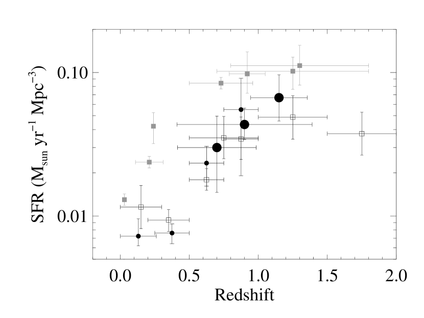
Using this conversion, we obtain a comoving density of star formation of M⊙ yr-1 Mpc-3 at . Figure 5 compares the SFR density to values measured from other rest-frame UV-optical surveys. The SPS value is calculated as an integral over a large redshift range (), but it can also be measured for a subset of the sample. In Figure 5, we show the SPS density of star formation for the subsets of the data in the ranges and , with median redshifts of 0.72 and 1.14, respectively. We do not plot the SFR density inferred by H99, but these authors note that their SFR density agrees with CFRS9.
5 Discussion
As expected, the SPS data show strong evolution in the density of star-formation over the range . Although the uncertainties are involved are large, the evolution observed is consistent with , the same as that computed by Tresse et al. (2002) for evolution in H. The same exponent is derived when the other [OII] measurements in Figure 5 are included. The value agrees with the wavelength-independent exponent of for a matter dominated flat Universe (Hogg 2002). However, Baldrey et al. (2002) set a strong upper limit on the exponent of at .
It is apparent from Figure 5 that the [OII] measurements of the SFR density do not agree with the H measurements any more than with those inferred from the UV continuum. The clear difference between the H and UV measurements is usually attributed to dust extinction (e.g. Yan et al. 1999), but at 3727 Å, the [OII] emission should be subject to less extinction from dust than the UV continuum. Furthermore, any difference in extinction between H and [OII] should have been included, to first order, in the calibration of the ratio of the lines by Jansen et al. (2001), as that ratio was derived empirically from typically metal rich galaxies. If more sensitive spectro-photometry were obtained for the SPS sample, it would be possible to recalculate the inferred H luminosities using reddening information in the Jansen et al. fit. It might be argued that the SPS selection effects favor more reddened objects, if reddening is greater in more compact starbursts, perhaps as a result of the greater concentration of gas and dust. The CFRS9 measurement, however, shows the same distinction, and that survey had very different selection criteria.
The disagreement between the [OII] and H values might be resolved if both are corrected for extinction. Gallego et al. (2002) find the extinction correction for [OII] to be a factor of ten on average, which brings their measurement of the local SFR density into agreement with the density inferred from H (Gallego et al. 1995). This value seems quite large, however, and does not agree with that used in other studies. Tresse et al. (2002) apply a factor of 2 extinction correction to H and only a factor of 3.6 to [OII], similar to Sullivan et al. (2000).
The uncertainties in the measurement of the SFR density are still large, and the number of objects with both [OII] and H line fluxes is still small. A direct approach to resolving the differences suggested by Figure 5 is additional multiwavelength study of consistent samples. At , these measurements require sensitive near-IR spectroscopy. Observations of that kind are possible and becoming more common (e.g. Pettini et al. 2001, Teplitz et al. 2000) from the ground, or soon with the refurbished NICMOS.
References
- (1)
- (2) Calzetti, D. 1997, AJ, 113, 162
- (3)
- (4) Cohen, J. G., Hogg, D. W., Blandford, R., Cowie, L. L., Hu, E., Songaila, A., Shopbell, P., & Richberg, K. 2000, ApJ, 538, 29
- (5)
- (6) Connolly, A. J., Szalay, A. S., Dickinson, M., Subbarao, M. U., & Brunner, R. J. 1997, ApJ, 486, L11
- (7)
- (8) Cowie, L. L., Songaila, A., Hu, E. M., & Cohen, J. G. 1996, AJ, 112, 839
- (9)
- (10) Gallego, J., Zamorano, J., Aragón-Salamanca, A., & Rego, M. 1995, ApJ, 455, L1
- (11)
- (12) Gallego, J., García-Dabó, C. E., Zamorano, J., Aragón-Salamanca, A.,& Rego, M. 2002, ApJ, 570, L1
- (13)
- (14) Gardner, J.P., et al. 1998, ApJ, 492, L99
- (15)
- (16) Glazebrook, K. Blake, C., Economou, F., Lilly, S., & Colless, M. 1999,& MNRAS,306, 843
- (17)
- (18) Hammer, F., et al. 1997, ApJ, 481, 49
- (19)
- (20) Hicks, E. K. S., Malkan, M. A., Teplitz, H. I., McCarthy, P. J., & Yan, L. 2002, ApJ in press
- (21)
- (22) Hogg, D. W., Cohen, J. G., Blandford, R., Pahre, M. A. 1999a, ApJ, 504, 622
- (23)
- (24) Hogg, D.W. 1999b, astro-ph, 9905116
- (25)
- (26) Hogg, D.W. 2002, ApJL, submitted; astro-ph, 0105280
- (27)
- (28) Hopkins, A. M., Connolly, A. J., & Szalay, A. S. 2000, AJ, 120, 2843
- (29)
- (30) Jansen, R. A., Franx, M., Fabricant, D. 2001, ApJ, 551, 825
- (31)
- (32) Kennicutt, R.C., Jr. 1992, ApJ, 338, 310
- (33)
- (34) Kennicutt, R. C., Jr. 1998, ARA&A, 36, 189
- (35)
- (36) Lilly,S.J., Tresse, L., Le Fèvre, O., Hammer, F., & Crampton, D. 1995, ApJ, 455, 108
- (37)
- (38) Lilly, S.J., Le Fevre, O., Hammer, F., & Crampton, D. 1996, ApJ, 460, L1
- (39)
- (40) Madau, P., Ferguson, H.C., Dickinson, M.E., Giavalisco, M., Steidel, C.C., & Fruchter, A. 1996, MNRAS, 283, 1388
- (41)
- (42) Madau, P., Pozzetti, L., Dickinson, M. 1998, ApJ, 498, 106
- (43)
- (44) McCarthy, P.J., et al. 1999, ApJ,520, 548
- (45)
- (46) Oke, J. B., et al. 1995, PASP, 107, 375
- (47)
- (48) Pascual, S., Gallego, J., Aragón-Salamanca, A., & Zamorano, J. 2001, A&A, 379, 798
- (49)
- (50) Pettini, M., Shapley, A.E., Steidel, C.C., Cuby, J.-G., Dickinson, M., Moorwood, A.F.M., Adelberger, K.L., & Giavalisco, M. 2001, ApJ, 554, 981
- (51)
- (52) Sullivan, M., Treyer, M. A., Ellis, R. S., Bridges, T. J., Milliard, B., Donas, J. 2000, MNRAS, 312, 442
- (53)
- (54) Teplitz, H.I, Collins, N.R, Gardner, J.P., Heap, S.R., Hill, R.S., Lindler, D.J., Rhodes, J., & Woodgate, B.E. 2002, ApJS submitted
- (55)
- (56) Teplitz, H.I., et al. 2000,ApJ, 533, L65
- (57)
- (58) Thompson, R. I., Rieke, M., Schneider, G., Hines, D. C., & Corbin, M. R. 1998, ApJ, 492, L95
- (59)
- (60) Tresse, L., & Maddox, S. J. 1998, ApJ, 495, 691
- (61)
- (62) Tresse, L., Maddox, S.J., Le Fevre, O., Cuby, J.-G. 2002, MNRAS in press; astro-ph, 0111390
- (63)
- (64) Treyer, M. A., Ellis, R. S., Milliard, B., Donas, J., & Bridges, T. J. 1998, MNRAS, 300, 303
- (65)
- (66) Williams, R.E. et al. 1996, AJ, 112,1335
- (67)
- (68) Yan, L., McCarthy, P.J., Freudling, W., Teplitz, H.I., Malumuth, E.M., & Weymann, R.J., Malkan, M.A. 1999, ApJ, 519, L47
- (69)
- (70)
| SNR | () | () |
|---|---|---|
| Completeness (%) | Completeness (%) | |
|
|
39 | 20 |
| 4 | 56 | 28 |
| 5 | 72 | 44 |
| 6 | 86 | 58 |
| 7 | 96 | 69
|