A Self-Consistent Study of Triaxial Black-Hole Nuclei

Abstract

We construct models of triaxial galactic nuclei containing central black holes using the method of orbital superposition, then verify their stability by advancing $N$-body realizations of the models forward in time. We assume a power-law form for the stellar density, $\rho\propto r^{-\gamma}$, with $\gamma=1$ and $\gamma=2$; these values correspond approximately to the nuclear density profiles of bright and faint galaxies respectively. Equidensity surfaces are ellipsoids with fixed axis ratios. The central black hole is represented by a Newtonian point mass. We consider three triaxial shapes for each value of $\gamma$: almost prolate, almost oblate and maximally triaxial. Two kinds of orbital solution are attempted for each mass model: the first including only regular orbits, the second including chaotic orbits as well. We find that stable configurations exist, for both values of $\gamma$, in the maximally triaxial and nearly-oblate cases; however steady-state solutions in the nearly-prolate geometry could not be found. A large fraction of the mass, of order 50% or more, could be assigned to the chaotic orbits without inducing evolution. Our results demonstrate that triaxiality may persist even within the sphere of influence of the central black hole, and that chaotic orbits may constitute an important building block of galactic nuclei.

Keywords: galaxies: elliptical and lenticular — galaxies: structure — galaxies: nuclei — stellar dynamics

1. Introduction

Schwarzschild (1979) demonstrated how to construct self-consistent models of stellar systems in the absence of analytic expressions for the orbital integrals. His method consists of three steps. i) Represent the stellar system by a smooth density law and divide it into discrete cells; ii) compute a library of orbits in the potential corresponding to the assumed density law, and record the time spent by each orbit in the cells; iii) find a linear combination of orbits that reproduces the cell masses. Using his method, Schwarzschild (1979, 1982) demonstrated self-consistency of triaxial mass models with and without figure rotation. Most of the orbits in his solutions were regular, i.e. non-chaotic (Merritt 1980). Subsequently, Statler (1987) found a variety of self-consistent solutions for the integrable, or “perfect,” triaxial mass models in which all orbits are regular.

Models like these with large, constant-density cores are now known to be poor representations of elliptical galaxies, almost all of which have high central densities (Crane et al. (1993); Ferrarese et al. 1994). Stellar densities rise toward the center approximately as power laws, $\rho\propto r^{-\gamma}$. Fainter galaxies have steeper cusps, $\gamma\approx 2$, while brighter galaxies have weaker cusps, $0\mathrel{\mathchoice{\lower 3.6pt\vbox{\halign{$\mathsurround=0pt\displaystyle\hfil#\hfil$\cr<\crcr\sim\crcr}}}{\lower 3.6pt\vbox{\halign{$\mathsurround=0pt\textstyle\hfil#\hfil$\cr<\crcr\sim\crcr}}}{\lower 3.6pt\vbox{\halign{$\mathsurround=0pt\scriptstyle\hfil#\hfil$\cr<\crcr\sim\crcr}}}{\lower 3.6pt\vbox{\halign{$\mathsurround=0pt\scriptscriptstyle\hfil#\hfil$\cr<\crcr\sim\crcr}}}}\gamma\mathrel{\mathchoice{\lower 3.6pt\vbox{\halign{$\mathsurround=0pt\displaystyle\hfil#\hfil$\cr<\crcr\sim\crcr}}}{\lower 3.6pt\vbox{\halign{$\mathsurround=0pt\textstyle\hfil#\hfil$\cr<\crcr\sim\crcr}}}{\lower 3.6pt\vbox{\halign{$\mathsurround=0pt\scriptstyle\hfil#\hfil$\cr<\crcr\sim\crcr}}}{\lower 3.6pt\vbox{\halign{$\mathsurround=0pt\scriptscriptstyle\hfil#\hfil$\cr<\crcr\sim\crcr}}}}1$, and exhibit an obvious break in the surface brightness profile. Following this discovery, Schwarzschild (1993) investigated triaxial models with singular density profiles, $\rho\sim r^{-2}$, and Merritt & Fridman (1996) constructed self-consistent solutions for triaxial galaxies with both weak and strong central cusps. A significant portion of the phase space in these models was found to be occupied by stochastic orbits. Furthermore, triaxial self-consistency could sometimes only be achieved by including some stochastic orbits. Models containing stochastic orbits can represent bona-fide equilibria as long as the stochastic orbits are represented as fully-mixed ensembles (Merritt & Fridman 1996; Merritt & Valluri 1996).

In the last decade, evidence has grown that supermassive black holes are generic components of galactic nuclei (Ho 1999). There are roughly a dozen galaxies in which a compelling case for the presence of a supermassive black hole can be made based on the kinematics of stars or gas (Merritt & Ferrarese 2001), as well as a number of active galactic nuclei in which the kinematics of the broad emission line region imply the existence of a supermassive black hole (Peterson 2002). Inferred masses range from $\sim 10^{6}{{\cal M}_{\odot}}$ to $\sim 10^{9.5}{{\cal M}_{\odot}}$ and correlate well with stellar velocity dispersions (e.g. Ferrarese et al. (2001)) and bulge luminosities (e.g. McLure & Dunlop (2002)).

The possibility of maintaining triaxiality within a galactic nucleus containing a supermassive black hole remains a topic of interest. Very close to the black hole, the gravitational force can be considered a perturbation to the Kepler problem and the phase space is essentially regular (Merritt & Valluri (1999); Sambhus & Sridhar (2000); Poon & Merritt (2001), hereafter Paper I). Farther from the black hole, the fraction of chaotic orbits increases, up to a radius where the enclosed stellar mass is a few times the black hole mass; beyond this radius essentially all centrophilic orbits are chaotic (Paper I). The tube orbits remain mostly regular since they avoid the destabilizing center. The persistence of regular orbits throughout the region where the gravitational force from the black hole dominates, leaves open the possibility of constructing self-consistent solutions. Furthermore there is growing observational evidence for the existence of bar-like distortions at the very centers of galaxies (e. g. Erwin & Sparke (2002)).

In Paper II (Poon & Merritt 2002), we presented preliminary results showing that self-consistent and stable triaxial equilibria could be constructed for power-law nuclei with certain axis ratios. In this paper, we present a more detailed investigation of triaxial black-hole nuclei. We find that stationary solutions are possible only for certain shapes; mass models that are too near to prolate axisymmetry always evolve toward axisymmetry.

The properties of the mass models are presented in §2. Orbital solutions for various shapes and density profiles are presented in §3 and their stability is tested by N-body simulation in §4 and §5. Limits on the chaotic mass fraction are discussed in §6. §7 discusses some implications for the nuclear dynamics of galaxies.

2. Mass Model

We model the stellar distribution by the density law:

$$\rho_{\star} = \rho_{\circ}m^{-\gamma},$$ (1)

$$m^{2} = \frac{x^{2}}{a^{2}}+\frac{y^{2}}{b^{2}}+\frac{z^{2}}{c^{2}},$$ (2)

The equidensity surfaces are concentric ellipsoids with fixed axis ratios $a:b:c$ and the radial profile is a power law with index $-\gamma$. We define the outer surface by the ellipsoid $m=m_{out}$ and measure the triaxiality via the index $T$, where:

$$T\equiv\frac{a^{2}-b^{2}}{a^{2}-c^{2}}.$$ (3)

Oblate and prolate galaxies have $T=0$ and $T=1$ respectively. $T=0.5$ corresponds to a “maximally triaxial” nucleus.

We consider two types of nuclei, the weak cusp ($\gamma=1$) and the strong cusp ($\gamma=2$), which correspond roughly to the density profiles observed at the centers of bright and faint elliptical galaxies respectively. For each value of $\gamma$, we consider three shapes: almost oblate ($T=0.25,a:b:c=1.0:0.9:0.5$); maximally triaxial ($T=0.50,a:b:c=1.0:0.79:0.5$); and almost prolate ($T=0.75$, $a:b:c=1.0:0.66:0.5$). All models have $c/a=0.5$.

The black hole is represented by a central point mass with $M_{bh}=1$, which imposes a scale to the otherwise scale-free stellar mass model. We define two characteristic radii associated with the presence of the black hole (Tables 1, 2). i) $r_{g}$ is defined such that the enclosed stellar mass within an ellipsoid with $m=r_{g}$ is equal to that of the black hole. For $T=0.5$, $r_{g}=0.64$ for $\gamma=1$ and $r_{g}=0.20$ for $\gamma=2$. ii) $r_{ch}$ is the radius beyond which the regular, boxlike orbits become almost all stochastic. For $T=0.50$, $r_{ch}\sim 2r_{g}$ for $\gamma=1$ and $r_{ch}\sim 6r_{g}$ for $\gamma=2$.

The gravitational potential can be obtained from Chandrasekhar’s theorem (Chandrasekhar (1969)), which is valid for density laws that are stratified on similar ellipsoids. The corresponding forces may be obtained in analytical form by taking partial derivatives of the potential. The details are given in §2 of Paper I.

Our orbital solutions require a finite outer radius. Our aim was to explore the possibility of maintaining triaxiality out to a radius of at least $r_{ch}$; hence we chose the outer surface of our model to be large enough that almost all of the density at $r_{ch}$ in a real galaxy would be contributed by orbits with apocenters $r_{+}$ lying below this surface.

To estimate $m_{out}$, we considered a spherical galaxy with density

$$\rho_{*}^{sph}=\rho_{\circ}r^{-\gamma}.$$ (4)

The isotropic distribution function corresponding to the density law (4) can be found using Eddington’s formula,

$$f^{sph}(E) = \frac{\sqrt{2}}{4\pi^{2}}\int_{E}^{a}\frac{d^{2}\rho_{*}^{sph}}{d\Phi^{2}}\frac{d\Phi}{\sqrt{\Phi-E}}$$ (5)

$$+ \frac{\sqrt{2}}{4\pi^{2}}\lim_{{\Phi}\to\Phi_{\infty}}\frac{d\rho_{*}^{sph}}{d\Phi}\frac{1}{\sqrt{\Phi-E}},$$

with $\Phi$ the potential generated by $\rho_{*}(r)$ and by the central point mass, and $\Phi_{\infty}\equiv\lim_{r\to\infty}\Phi(r)$. We then change variables such that

$$d\rho^{sph}_{*}=\frac{2\pi}{r^{2}}\frac{f_{\star}^{sph}}{v_{r}}\Biggl{|}\frac{\partial(E,L^{2})}{\partial(r_{+},r_{-})}\Biggr{|}dr_{+}dr_{-},$$ (6)

with $v_{r}=\sqrt{2(E-L^{2}/2r^{2}-\Phi(r)}$ the radial velocity, and $r_{+}$ and $r_{-}$ the apocenter and pericenter of an orbit with energy $E$ and angular momentum $L$. The Jacobian is

$$\frac{\partial(E,L^{2})}{\partial(r_{+},r_{-})}\equiv\left|\frac{\partial E}{\partial r_{+}}\frac{\partial L^{2}}{\partial r_{-}}-\frac{\partial E}{\partial r_{-}}\frac{\partial L^{2}}{\partial r_{+}}\right|.$$ (7)

According to (6), we define

$$g(r_{+},r)\equiv\int_{0}^{r_{+}}\frac{2\pi}{r^{2}}\frac{f_{\star}^{sph}}{v_{r}}\Biggl{|}\frac{\partial(E,L^{2})}{\partial(r_{+},r_{-})}\Biggr{|}dr_{-},$$ (8)

$$u(r_{+},r)\equiv\frac{1}{\rho^{sph}_{*}(r)}\int_{0}^{r_{+}}g(r_{+},r)dr_{+}.$$ (9)

$u(r_{+},r)$ is the fraction of the mass at $r$ contributed by orbits with apocenters $r\leq r_{+}$.

                                                                      

$u(r_{+},r)$ as a function of $r_{+}/r$ for $\gamma=1$ and $2$ and for different radii, as indicated.

Figure 2 plots $u(r_{+},r)$ as a function of $r_{+}/r$ for both weak and strong cusp nuclei. The red curves correspond to infinite $r$, i.e. no influence from the black hole. The black curves correspond to very small $r$, where the potential is almost Keplerian. $u(r_{+},r)$ for the weak cusp case is smaller than that for the strong cusp at a given $r_{+}/r$, because the density of the strong cusp falls off faster, thus the mass at a given $r$ has to rely more heavily on nearby orbits.

Based on these results, we took $m_{out}$ to be $5r_{ch}$ for $\gamma=1$ and $3r_{ch}$ for $\gamma=2$, so that about $70\%(75\%)$ of the mass at $r_{ch}$ is accounted for in the weak (strong) cusp cases respectively. Tables 2 and 2 give the values of the characteristic radii in model units.

Table 1Model Parameters for $\gamma=1$

	$~{}~{}T=0.25~{}~{}$	$~{}~{}T=0.50~{}~{}$	$~{}~{}T=0.75~{}~{}$
$r_{g}$	$0.594$	$0.635$	$0.694$
$r_{ch}$	$1.057$	$1.128$	$1.234$
$m_{out}$	$5.284$	$5.642$	$6.168$

Table 2Model Parameters for $\gamma=2$

	$~{}~{}T=0.25~{}~{}$	$~{}~{}T=0.50~{}~{}$	$~{}~{}T=0.75~{}~{}$
$r_{g}$	$0.177$	$0.201$	$0.241$
$r_{ch}$	$1.114$	$1.270$	$1.518$
$m_{out}$	$3.342$	$3.811$	$4.555$

3. Construction of Orbital Solutions

We followed standard procedures for constructing the Schwarzschild solutions. The cells used to define the mass distribution were defined as follows. Each model with outer surface $m_{out}$ was divided into 64 shells. The inner 63 shells were equidensity surfaces; the outermost shell was an equipotential surface, in order to accomodate chaotic orbits which fill regions defined by equipotential surfaces. Shells were more closely spaced near the center. The $42$nd shell in each model corresponded to $r_{ch}$. Each shell was further divided into 48 angular cells per octant as Merritt & Fridman (1996), giving a total of 3072 cells per octant. Due to the symmetry of the problem, it is necessary to consider only a single octant when constructing the orbital solutions.

Orbits were computed in two initial condition spaces: stationary start space, which yields mostly centrophilic orbits (pyramids, stochastic orbits); and $X-Z$ start space, which yields mostly tube orbits. Orbital energies were selected from a grid of 42 (52) values for $\gamma=1$ (2), defined as the energies of equipotential surfaces which were spaced similarly in radius to the equidensity shells. The outermost energy shell, which is also an equipotential surface, intersects the $x$-axis at $x=m_{out}$ for both mass models. $X-Z$ start space consists of orbits which begin on the $X$-$Z$ plane with $v_{x}=v_{z}=0$; stationary start space consists of orbits which begin with zero velocity. A total of 18144 (22464) orbits were integrated for 100 dynamical times for $\gamma=1(2)$ and their contributions to the masses in the cells were recorded. In order to distinguish regular from stochastic trajectories, the largest Liapounov exponent was computed for each orbit.

Twelve equations – six representing the unperturbed motion and six the linearized perturbations – were integrated using the routine RADAU of Hairer (1996), which is a variable time step, implicit Runge-Kutta Scheme which automatically switches between orders of 5, 9, and 13. Energy was typically conserved to a few parts in $10^{9}$ over 100 orbital periods.

An orbit was considered regular if the largest Liapunov exponent $\lambda$ satisfied $\lambda T_{D}<10^{-0.9}$. The dynamical time $T_{D}$ is defined as the period of a circular orbit of the same energy in the equivalent spherical potential, which is defined to have a scale length $(abc)^{\frac{1}{3}}$ (Paper I). This threshold was determined empirically by making histograms of Liapounov exponents of mono-energetic orbits at various energies; $\lambda T_{D}\approx 10^{-0.9}$ was found to always separate the two peaks in the histogram corresponding to regular and chaotic orbits. A large fraction of the computed orbits were found to be stochastic, as shown in Table 3.

Table 3Fraction of regular orbits in the orbit libraries

	$~{}~{}~{}~{}~{}~{}~{}\gamma=1~{}~{}~{}~{}~{}~{}~{}$	$~{}~{}~{}~{}~{}~{}~{}\gamma=2~{}~{}~{}~{}~{}~{}~{}$
$~{}~{}T=0.25~{}~{}$	$0.58$	$0.72$
$~{}~{}T=0.50~{}~{}$	$0.54$	$0.67$
$~{}~{}T=0.75~{}~{}$	$0.49$	$0.65$

We then found the linear combination of orbits which best reproduced the cell masses. We did this by varying the orbital occupation numbers $C_{i}$ to minimize the quantity $\chi^{2}$, defined as:

$$\chi^{2}=\sum_{l=1}^{N}(D_{l}-\sum_{i=1}^{M}B_{li}C_{i})^{2}.$$ (10)

$B_{li}$ is the time spent by the $i$-th orbit in the $l$-th cell, $D_{l}$ is the mass of the $l$-th cell, and $C_{i}$ is the occupation number of the $i$-th orbit. The quadratic programming problem was solved using the NAG Fortran library routine E04NFC. We measured the discrepancies of the orbital solutions by the parameter:

$$\Delta^{2}=\frac{1}{N}\sum_{l=1}^{N}(1-\frac{1}{D_{l}}\sum_{i=1}^{M}B_{li}C_{i})^{2},$$ (11)

the mean error in the cell masses.

We constructed two solutions for each mass model: one using only regular orbits, and the other using both regular and chaotic orbits. Schwarzschild (1993) was the first to include chaotic orbits in self-consistent solutions. Schwarzschild treated the chaotic orbits like regular orbits, giving each chaotic orbit its own occupation number, even though many of the chaotic orbits in his models were “sticky” and did not reach a time-averaged steady state during the interval of integration. He justified this practice by re-integrating all chaotic orbits with non-zero occupation numbers for longer intervals in the fixed potential; the extreme error in the cell masses was found to increase from the original $\sim 1\%$ to $\sim 10\%$. Merritt & Fridman (1996) noted that fully-mixed chaotic orbits, i.e. chaotic orbits that uniformly fill their accessible phase space region, are bona-fide building blocks for steady-state galaxies and approximated such building blocks by constructing ensemble averages of the chaotic orbits at each energy.

We followed Schwarzschild in allowing different chaotic orbits at a given energy to have different occupation numbers. In our potentials, the chaotic orbits were observed to very quickly fill the region accessible to them: their “mixing times” were generally much shorter than the integration interval. Hence we expected that our chaotic orbits would individually constitute bona fide building blocks for a stationary solution, without the need to construct ensemble averages as in Merritt & Fridman (1996). This expectation was confirmed by the $N$-body integrations described below.

                                                                      

Schematic diagram showing the three kinds of shells used for constraining the orbital solutions. (i) The innermost shells with all angular constraints imposed. (ii) Intermediate shells with angular constraints ignored. (iii) The outermost shells, which are ignored. The highest-energy shell is an equipotential surface while the other shells are equidensity ellipsoids.

We could not find quadratic-programming solutions which exactly reproduced the cell masses in all of the cells, including the outermost ones. This is probably because the number of orbits visiting the outer shells is small, giving the quadratic programming algorithm little freedom to fit the cell masses there. Indeed in all of our self-consistent solutions, most of the contribution to $\Delta^{2}$ came from the outermost cells. We therefore considered solutions in which the outermost cells were treated in various ways. Figure 3 illustrates the idea. We defined three kinds of mass shells: (i) the innermost shells with all the constraints imposed, i.e. all of the angular cells included; (ii) intermediate shells for which only the total mass was fit, with angular details ignored; (iii) the outermost shells which were excluded from the fit. We carried out numerous tests in which we attempted to fit various combinations of constraints. As expected, the discrepancy $\Delta$ defined by the innermost shells always decreased as the total number of constraints decreased. For instance, for the weak cusp model with $T=0.50$, including all the orbits allowed the innermost $60$ shells ($r\sim 4r_{ch}$) to be fit to machine precision when the outermost four shells were ignored. When these “exact” solutions were advanced forward in time, however, they were found to exhibit significant evolution at large radii, due presumably to the poor fit in the outermost cells. We discuss this further in §5. Experiments like this persuaded us to focus on solutions that were not “exact” but rather were constrained to reproduce the densities in all cells within $m_{out}$ to as high an accuracy as possible. Such solutions exhibited smaller fractional errors in the inner cells ($r\mathrel{\mathchoice{\lower 3.6pt\vbox{\halign{$\mathsurround=0pt\displaystyle\hfil#\hfil$\cr<\crcr\sim\crcr}}}{\lower 3.6pt\vbox{\halign{$\mathsurround=0pt\textstyle\hfil#\hfil$\cr<\crcr\sim\crcr}}}{\lower 3.6pt\vbox{\halign{$\mathsurround=0pt\scriptstyle\hfil#\hfil$\cr<\crcr\sim\crcr}}}{\lower 3.6pt\vbox{\halign{$\mathsurround=0pt\scriptscriptstyle\hfil#\hfil$\cr<\crcr\sim\crcr}}}}r_{ch}$) than in the outer ones. Models constructed in this way were found to evolve much less than the “exact” solutions and provide the basis for the discussion below.

The orbital content and the precision $\Delta$ of the solutions are represented in various ways in Tables 3-3 and in Figures 1-2. We classify orbits into one of four families (cf. Paper I). $x$- and $z$-tubes are regular orbits that circulate around the long and short axes of the figure, respectively. Pyramid orbits are the closest analogs to box orbits in these potentials; they can be described as eccentric Keplerian ellipses that precess due to torques from the stellar potential. Their major elongation is contrary to that of the figure. We will indiscriminately refer to these orbits as “pyramids” and “box orbits” in what follows. The fourth family consists of the chaotic orbits.

Tables 3 - 3 give the mass fractions within various radii contributed by the four types of orbit. $z$-tube orbits (short-axis tubes) are the biggest contributors in all of the regular-orbit solutions, making up at least $50\%$ of the total mass and as much as 80% in the nearly-oblate ($T=0.25$) models. Pyramid orbits are next in importance; their contribution reaches $\sim 40\%$ for $\gamma=1$ and $\sim 15\%$ for $\gamma=2$. $x$-tubes (long-axis tubes) are relatively unimportant in the models with $T=0.25$ and $0.5$, making up only a few percent of the total mass. In the nearly prolate models ($T=0.75$), their contribution increases to $\sim 20\%$, however we argue below that these prolate solutions do not represent true equilibria.

When chaotic orbits are included in the orbit libraries, the character of the solutions changes substantially: at least $40\%$ of the mass is assigned to chaotic orbits by the quadratic programming algorithm, and as much as $60\%$ in the models with $\gamma=1$ and $T=(0.25,0.5)$. The inclusion of chaotic orbits lowers the mean error $\Delta$ by a modest amount in both the weak and strong cusp cases (Tables 4-6). Much of the mass assigned to the chaotic orbits appears to be “taken” from the pyramid orbits, as expected. To our knowledge, these solutions contain a larger fraction of chaotic orbits than in any other self-consistent galaxy models. Since the time-averaged shapes of the chaotic orbits are nearly spherical, the existence of these solutions implies that the regular orbits have more than enough freedom to reproduce the triaxial shapes, and can do so even when forced to compensate for the inauspicious shapes of the chaotic orbits.

Another way to represent the orbital makeup of the solutions is via the distribution of orbital energies. Let $M_{i}(E)dE$ be the mass in orbits from the $i$th orbital family whose energies lie in the range $E$ to $E+dE$. The cumulative mass is given by $M_{i}(<E)=\int^{E}_{-\infty}M_{i}(E)dE$. Figure 1 shows $M_{i}(<E)$ for the self-consistent solutions with $T=0.5$. We show for comparison $M^{sph}(<E)$ computed for the equivalent spherical models defined in the Appendix. One expects that $M^{sph}(<E)\approx\sum_{i}M_{i}(<E)$, and Figure 1 verifies that this is correct. At high energies, there are discrepancies between the Schwarzschild solutions and the predictions of the spherical models. This is because the Schwarzschild solutions are truncated; thus, orbits with the highest energies are forced to make large contributions, which in turn lowers the contributions from orbits at lower energies. This effect is more significant for the weak cusp models which place most of their mass at large radii. Nevertheless, at low energies even the $\gamma=1$ solutions have nearly the same $M(<E)$ dependence as the equivalent spherical models.

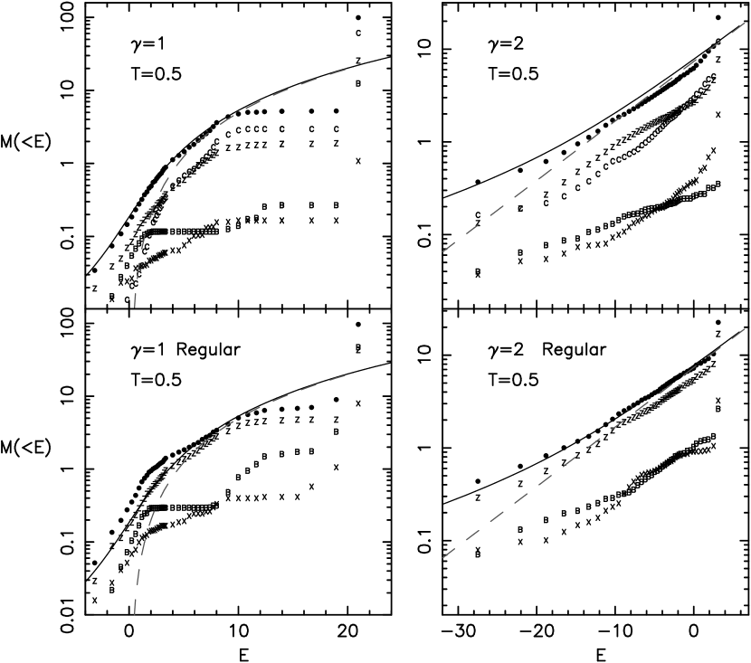
Figure 1.— Cumulative energy distributions of the various orbital families, in self-consistent solutions with $T=0.5$. The symbols “B”, “X”, “Z”, “C” denote the mass contributed by box, $x$-tube, $z$-tube and chaotic orbits respectively; black dots give the total. Solid (dotted) lines show $M(<E)$ for the equivalent spherical models defined in the Appendix, with (without) the central black hole.

Table 4Orbital Content of Solutions with $T=0.25$

	$z$-tubes	$x$-tubes	pyramids	chaotic
$\gamma=1:$ (regular)
$\log(\Delta)=-1.115$
$r<0.5$	0.70	0.06	0.24	—
$r<1.0$	0.62	0.06	0.33	—
$r<1.5$	0.59	0.05	0.36	—
$\gamma=1:$ (all)
$\log(\Delta)=-1.318$
$r<0.5$	0.40	0.03	0.07	0.50
$r<1.0$	0.34	0.02	0.06	0.59
$r<1.5$	0.30	0.01	0.06	0.63
$\gamma=2:$ (regular)
$\log(\Delta)=-1.437$
$r<0.4$	0.81	0.07	0.11	—
$r<0.8$	0.80	0.08	0.12	—
$r<1.2$	0.80	0.08	0.12	—
$\gamma=2:$ (all)
$\log(\Delta)=-2.633$
$r<0.4$	0.56	0.03	0.07	0.34
$r<0.8$	0.55	0.03	0.07	0.35
$r<1.2$	0.53	0.03	0.07	0.37

Table 5Orbital Content of Solutions with $T=0.50$

	$z$-tubes	$x$-tubes	pyramids	chaotic
$\gamma=1:$ (regular)
$\log(\Delta)=-1.169$
$r<0.5$	0.64	0.13	0.23	—
$r<1.0$	0.56	0.08	0.36	—
$r<1.5$	0.52	0.07	0.41	—
$\gamma=1:$ (all)
$\log(\Delta)=-1.307$
$r<0.5$	0.29	0.07	0.11	0.54
$r<1.0$	0.27	0.03	0.10	0.60
$r<1.5$	0.25	0.02	0.10	0.62
$\gamma=2:$ (regular)
$\log(\Delta)=-1.295$
$r<0.4$	0.73	0.11	0.16	—
$r<0.8$	0.73	0.11	0.15	—
$r<1.2$	0.73	0.12	0.15	—
$\gamma=2:$ (all)
$\log(\Delta)=-2.567$
$r<0.4$	0.46	0.05	0.09	0.40
$r<0.8$	0.45	0.05	0.06	0.44
$r<1.2$	0.44	0.05	0.05	0.46

Table 6Orbital Content of Solutions with $T=0.75$

	$z$-tubes	$x$-tubes	pyramids	chaotic
$\gamma=1:$ (regular)
$\log(\Delta)=-1.379$
$r<0.5$	0.44	0.27	0.29	—
$r<1.0$	0.48	0.20	0.32	—
$r<1.5$	0.47	0.16	0.37	—
$\gamma=1:$ (all)
$\log(\Delta)=-1.248$
$r<0.5$	0.27	0.14	0.16	0.42
$r<1.0$	0.26	0.07	0.14	0.53
$r<1.5$	0.22	0.06	0.16	0.56
$\gamma=2:$ (regular)
$\log(\Delta)=-1.221$
$r<0.4$	0.57	0.20	0.23	—
$r<0.8$	0.59	0.21	0.20	—
$r<1.2$	0.58	0.22	0.20	—
$\gamma=2:$ (all)
$\log(\Delta)=-2.471$
$r<0.4$	0.38	0.13	0.11	0.38
$r<0.8$	0.35	0.12	0.09	0.44
$r<1.2$	0.33	0.13	0.08	0.46

Figure 2 presents yet another representation of the orbital populations of our self-consistent solutions. We plot the cumulative mass fraction $F$ contributed by different kinds of orbits to different shells of the model. Box-orbits are blue, tube orbits are orange and chaotic orbits are purple; higher-energy orbits are represented by darker shades. Color bars relate the shades to the energy of the orbits. Numbers below the color bar indicate radii where the equidensity shells and equipotentials intersect the $x$-axis; note that the scale is not linear due to the higher resolution at lower radii. For instance, in the weak cusp model with $T=0.50$, shell 20 is an equidensity ellipsoid with $x$-intercept $0.78$, and regular box orbits with energy $E=\Phi(0.78,0.0,0.0)$ are represented by the lightest blue color.

At low energies, many of the $z$-tube orbits appear as saucers, i.e. $2:1$ resonant orbits; at high energies, higher-order resonances are important for these orbits. It is surprising that $x$-tube orbits do not dominate the nearly-prolate solutions with $T=0.75$. However configuration-space plots of the $x$-tube orbits show that almost all of them are elongated contrary to the prolate figure: they are thin circular rings lying near the $y-z$ plane. Even in the nearly-prolate solutions, most of the mass is contributed by $z$-tube orbits; the remaining contributions are mostly from high-energy box orbits, many of them associated with resonances. In the nearly-prolate solutions, the most important resonances are the “fish” ($2:3$) and the “pretzels” ($3:4$). In the nearly-oblate solutions, the fish and the “banana” ($2:1$) resonances dominate. Many of the $z$-tubes and the high-energy boxes are replaced after the introduction of chaotic orbits (Figure 2).

As discussed in more detail below, we were not able to predict the long-term stability of a model based on its value of $\Delta$. Some models with fairly large $\Delta$’s were found to exhibit almost no evolution, while other models with smaller $\Delta$’s evolved significantly. This suggests that the results of Schwarzschild modelling should be interpreted with caution in cases where the long-term stability of the solution has not been tested.

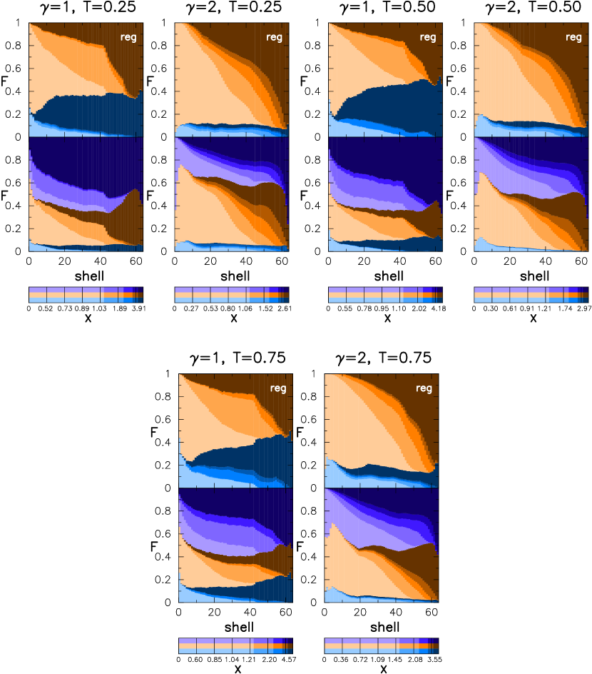
Figure 2.— Cumulative mass fraction $F$ contributed by different kinds of orbits to different shells of the triaxial solutions. Box orbits are blue, tube orbits (both $z$- and $x$-tubes) are orange, and chaotic orbits are purple. Higher energies are represented by darker shades, defined according to the $x$-intercept of the equipotential that has the same energy as the orbit. Numbers below the color bar indicate radii where the equidensity shells intersect the $x$-axis. Figures labelled “reg” respresent solutions constructed only using regular orbits.

4. $N$-body models

Each of the solutions described above was found via a minimization of the quantity $\chi^{2}$ describing the sum of the squared errors in the cell masses (equation 10). While the magnitude of $\chi^{2}$ might be expected to correlate with the quality of the solution, there is really no way to know how small $\chi^{2}$ must be in order for the solution to represent a bona fide steady state, or how large a value of $\chi^{2}$ is consistent with the existence of a smooth equilibrium solution. One could require that each of the cell masses be fit exactly; but we were never able to do this when the outermost shells were included, and in any case, the discrete representation of the density renders the interpretation of an “exact” solution problematic. There are other uncertainties as well; for instance, both “sticky” chaotic orbits and nearly-resonant, regular orbits may require very long integration times before their cell masses approximate the steady-state values.

We tested whether our orbital superpositions represent true equilibria by realizing them as $N$-body models and integrating them forward in time in the gravitational potential computed from the $N$ bodies themselves, and from a point mass representing the black hole. We prepared initial conditions corresponding to each of the orbital solutions by re-integrating orbits with non-zero occupation numbers and storing their positions and velocities at fixed time intervals. The sense of rotation of the tube orbits was chosen randomly. We used $\sim 2\times 10^{6}$ particles for representing the weak-cusp models and $\sim 2\times 10^{5}$ particles for the strong-cusp models; a smaller $N$ was chosen for $\gamma=2$ since the $N$-body integrations were slower for the more condensed model. We integrated the initial conditions forward in time using GADGET (Springel, Yoshida & White (2001)), a parallel tree code with variable time steps. The particle representing the black hole was allowed to move in response to the forces from the “stars.” The softening length was $0.005(0.003)$ for the weak (strong) cusp cases. Energy was conserved to within $\sim 0.5\%$ for the weak cusp models and $\sim 1\%$ for the strong cusp models.

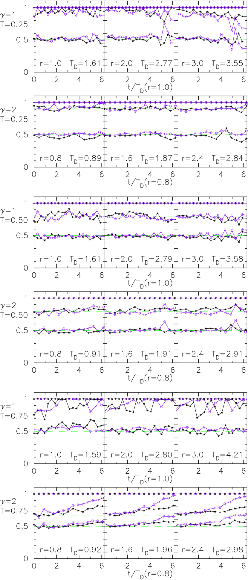
Figure 3.— Evolution of the axis lenghts at different radii for the orbital solutions shown in Figure 2. The longest axis is defined to have unit length. Black (purple) curves correspond to solutions containing only regular (both regular and chaotic) orbits. Green lines indicate the values of the axis lengths in the underlying mass models.

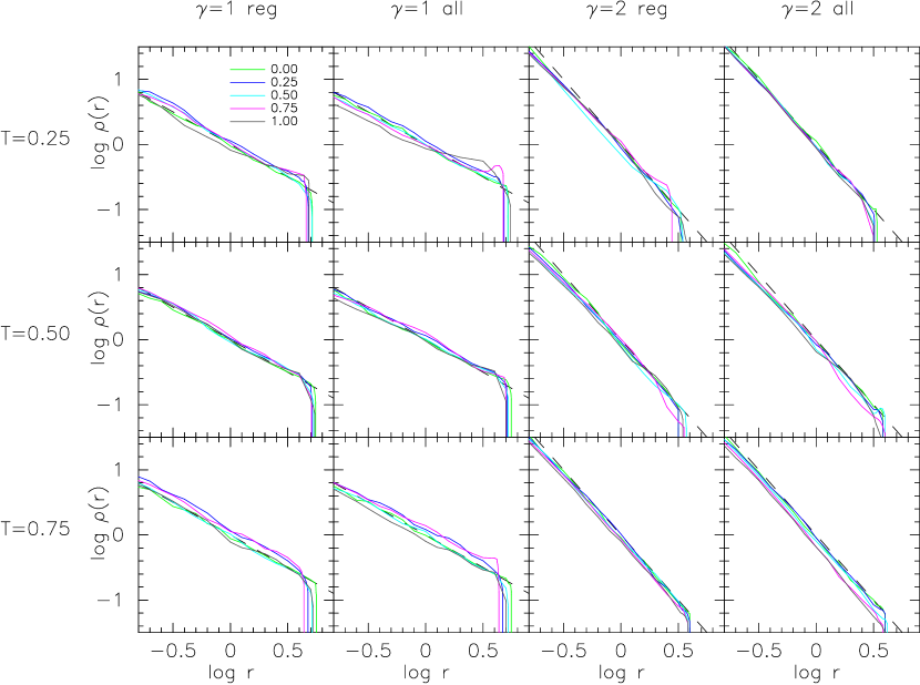
Figure 4.— Evolution of density profiles for the orbital solutions of Figure 2. Different colored curves correspond to the times shown in the upper left-hand panel, in units of the total integration time. Dotted lines are the density profile of the underlying mass model.

As our primary index of evolution, we computed the axis ratios of the models as a function of radius using the iterative procedure described by Dubinski & Carlberg (1991), as follows. (i) The moment of inertia matrix of the particles enclosed by a sphere of radius $r$ is calculated. (ii) Axis ratios are assigned as $a=\sqrt{m_{11}/m_{max}}$, $b=\sqrt{m_{22}/m_{max}}$, $c=\sqrt{m_{33}/m_{max}}$, where $m_{ii}$ are the principal moments of inertia and $m_{max}=\mbox{max}\{m_{11},~{}m_{22},~{}m_{33}\}$. (iii) Particles are enclosed within the ellipsoid $x^{2}/a^{2}+y^{2}/b^{2}+z^{2}/c^{2}=r^{2}$ and step (ii) is iterated, until the axis ratios converge.

Figures 3 and 4 show the evolution of the axis ratios and density profiles of the various solutions. None of the density profiles showed signficant evolution: the radial distribution of mass did not evolve for any of the models. However some of the solutions showed significant evolution in their shapes. For $T=0.5$ (maximum triaxiality) and $\gamma=(1,2)$, we observed no significant evolution in the axis ratios, either for the regular-orbit solutions or the solutions containing chaotic orbits. We conclude that the maximally-triaxial solutions represent bona-fide equilibria. For the weak-cusp model with $T=0.25$ (nearly oblate), there is some evolution at late times in the large-radius axis ratios, while the nearly-oblate model with $\gamma=2$ hardly evolves. Contour plots of the particle distribution suggest that the evolution for $\gamma=1$ is due to the relatively large errors in the cell masses at large radii; as time goes on these errors propagate to smaller radii. In spite of these fluctuations, however, we judged both of the $T=0.25$ solutions to be stable.

Figure 5.— Contours of the projected density of the solution with $\gamma=1$, $T=0.50$ and only regular orbits. The upper panels show the contours at $t=0$, and the lower panels show the contours at the end of the integration. This model was judged stable based on the lack of significant time evolution of the axis ratios (Figure 5); note the slight evolution of the contour shapes at the largest radii.

By contrast, all solutions with $T=0.75$ (nearly prolate) were found to exhibit substantial evolution, reaching nearly axisymmetric (oblate) shapes by the final time step. (We note that for the weak-cusp solution with $T=0.75$, even the initial, intermediate-to-long axis ratio deviated noticeably from that of the assumed mass model.) We were unable to find any solutions with $T=0.75$ that did not evolve toward complete axisymmetry. We conclude that these solutions do not represent bona-fide equilibria.

Figure 5 shows contours of the projected density of the weak cusp models with $T=0.50$ and only regular orbits. The contours remain approximately ellipsoidal until the end of the integration.

5. A model with outer angular constraints relaxed

We mentioned above that relaxing the angular constraints in the outermost shells led to quadratic programming solutions with very small errors in the innermost mass cells. However these solutions generally exhibited large changes in their shapes when evolved forward. We illustrate this in the case of a weak cusp nucleus with $T=0.50$ and only regular orbits. In the orbital solution for this model, we relaxed the angular constraints in the outer 5 shells, i.e. only the masses of these shells were fit by the quadratic programming routine, not the individual cell masses. By relaxing the outermost angular constraints, we were able to find a solution in which $\log(\Delta)=-2.1$ for the inntermost shells. Figure 6 shows the evolution of axis lengths of the model. The axis ratios show large fluctuations, especially at large radii. Figure 7 shows contours of the projected density. At $t=0$, the contours are ellipsoidal only at small radii; the large-radius contours are irregular due to the large cell mass discrepancies in the outer shells. During the integration, this model shows significant evolution at large radii, which in turn affects the contours at small radii. The final model looks very different from the initial model. We found similar behavior in other orbital solutions when the outermost constraints were relaxed.

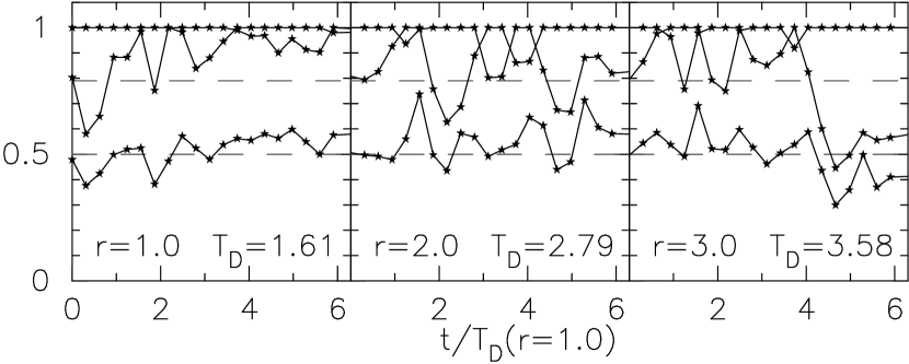
Figure 6.— Evolution of axis ratios of the weak cusp solution with the angular constraints on the outer five shells relaxed.

Figure 7.— Contours of the projected density of the weak cusp solution with $T=0.50$ and only regular orbits. The angular constraints of the 5 outer shells are ignored. The upper panels show the contours at $t=0$, and the lower panels show the contours at the end of the integration.

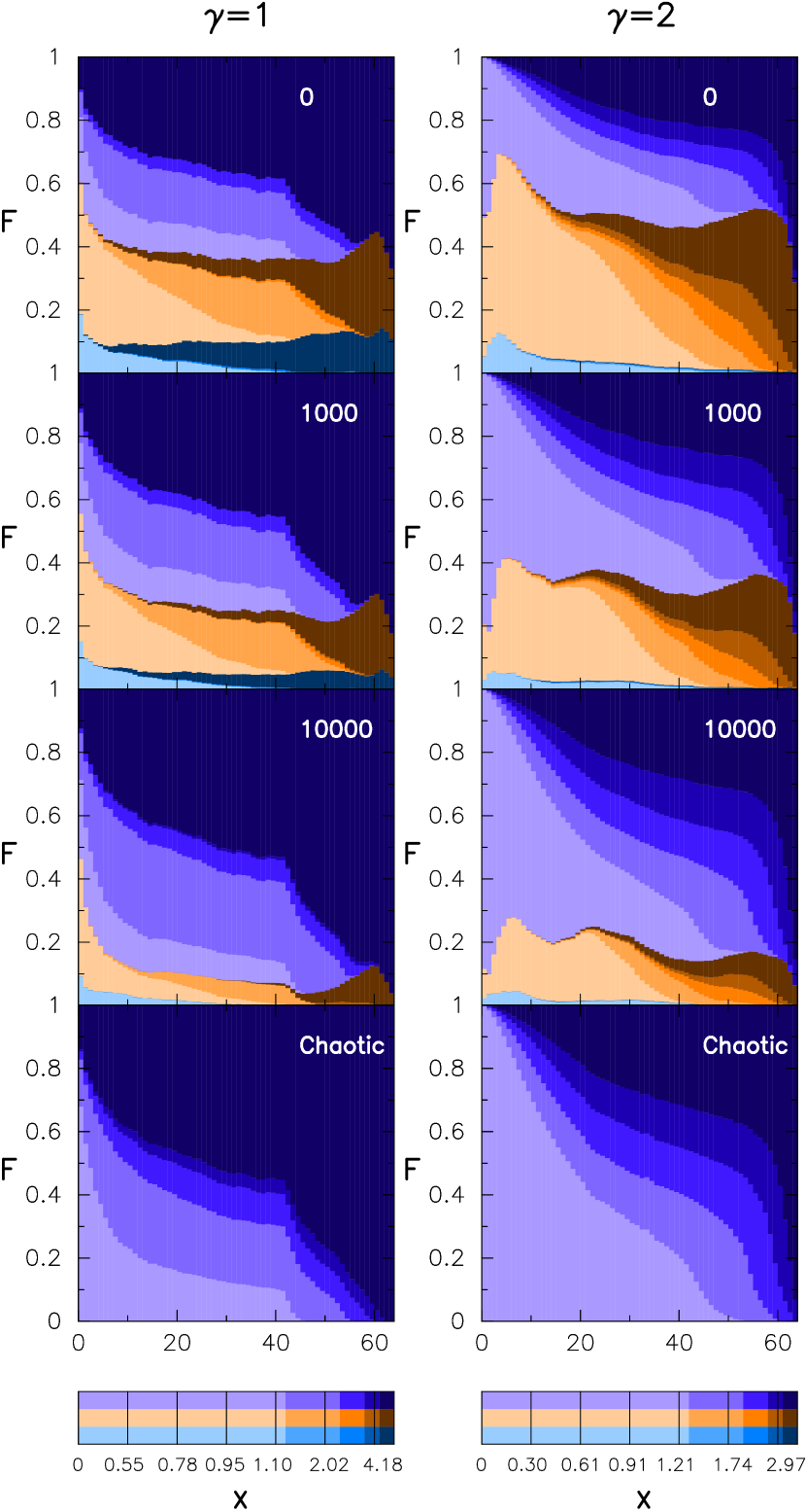
Figure 8.— Cumulative mass fractions $F$ contributed by different kinds of orbits to different shells of the triaxial solutions in which the contribution from chaotic orbits has been maximized. The value of $W_{C}$ is indicated in the upper right hand corner. Left column: $T=0.5,\gamma=1$. Right column: $T=0.5,\gamma=2$.

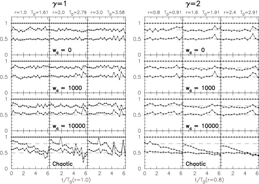
Figure 9.— Evolution of the axis ratios of the orbital solutions illustrated in Figure 8. Columns on the left show models with $\gamma=1,T=0.50$ and various values of $W_{C}$ at $r=1.0$ (first column), $r=2.0$ (second column), and $r=3.0$ (third column). Columns on the right show models with $\gamma=2,T=0.50$.

Figure 10.— Contours of the projected density of the weak cusp model with $T=0.50$ and $W_{C}=10000$. The upper panels show the contours at $t=0$, and the lower panels show the contours at the end of the integration.

6. Maximizing the contribution from Chaotic Orbits

The existence of long-lived triaxial models containing an abundance of chaotic orbits is particularly interesting: stars on such orbits pass once per crossing time near the center, greatly increasing the rate of interactions with the black hole compared with spherical or axisymmetric models. We sought to maximize the chaotic content in our models by minimizing the quantity:

$$\chi^{2}=\sum_{l=1}^{N}(D_{l}-\sum_{i=1}^{M}B_{li}C_{i})^{2}+\sum_{i=1}^{M}W_{i}C_{i}$$ (12)

instead of (10). Here $W_{i}$ is the “penalty” associated with the $i$th orbit; increasing $W_{i}$ tends to decrease the contribution $C_{i}$ from the $i$th orbit in the solution. We set $W_{i}=0$ for the chaotic orbits and $W_{i}\equiv W_{C}=(0,1000,10000)$ for the regular orbits. As $W_{C}$ increases, we expect the contribution from chaotic orbits to increase, although possibly at the expense of the overall quality of the fit to the cell masses. We also constructed solutions containing only chaotic orbits.

Figure 8 and Table 6 show the orbital content for weak and strong cusp solutions with $T=0.50$ and different values of $W_{C}$. The bottom panel of Figure 8 shows solutions containing only chaotic orbits. As $W_{C}$ increases, the regular orbits are replaced by high energy (low energy) chaotic orbits in the weak (strong) cusp solutions. Evolution of the axis-ratios is shown in Figure 9. Remarkably, only the models constructed from purely chaotic orbits show substantial evolution in their axis ratios. Inspection of the contour plots (e.g. Figure 10) does reveal some evolution away from elliptical isophotes in the solutions with large $W_{C}$, but the triaxiality appears robust. We conclude that chaotic mass fractions as large as $\sim 75\%$ or more might be consistent with long-lived triaxiality in galactic nuclei.

Table 7Orbital Content of Solutions with $T=0.5$ and Different $W_{C}$

	$z$-tubes	$x$-tubes	pyramids	chaotic
$\gamma=1:W_{C}=0$
$r<0.5$	0.29	0.07	0.11	0.54
$r<1.0$	0.27	0.03	0.10	0.60
$r<1.5$	0.25	0.02	0.10	0.62
$\gamma=1:W_{C}=1000$
$r<0.5$	0.24	0.06	0.09	0.61
$r<1.0$	0.21	0.03	0.06	0.70
$r<1.5$	0.20	0.02	0.06	0.73
$\gamma=1:W_{C}=10000$
$r<0.5$	0.14	0.05	0.05	0.76
$r<1.0$	0.09	0.02	0.03	0.87
$r<1.5$	0.07	0.01	0.01	0.91
$\gamma=2:W_{C}=0$
$r<0.4$	0.46	0.05	0.09	0.40
$r<0.8$	0.45	0.05	0.06	0.44
$r<1.2$	0.44	0.05	0.05	0.46
$\gamma=2:W_{C}=1000$
$r<0.4$	0.26	0.04	0.04	0.65
$r<0.8$	0.30	0.03	0.03	0.64
$r<1.2$	0.30	0.02	0.03	0.65
$\gamma=2:W_{C}=10000$
$r<0.4$	0.15	0.03	0.03	0.79
$r<0.8$	0.18	0.01	0.02	0.78
$r<1.2$	0.17	0.01	0.02	0.79

7. Summary and Discussion

We have shown that long-lived triaxial configurations are possible for nuclei containing black holes. Models with $T=0.5$ (maximally triaxial) and $T=0.25$ (oblate/triaxial) were constructed and found to be stable, retaining their non-axisymmetric shapes until the end of the integration interval, equal to several crossing times. Models with $T=0.75$ (prolate/triaxial) were always found to evolve rapidly to axisymmetry; we speculate that prolate/triaxial nuclei do not exist. The evolution seen in the nearly-prolate models does not appear to be a consequence of orbital chaos; indeed, in our stable solutions, we were able to replace a surprisingly large fraction of the regular orbits by chaotic orbits without inducing noticeable evolution in their shapes. We found that at least 50%, and perhaps as much as 75%, of the mass could be placed on chaotic orbits in the maximally triaxial and oblate/triaxial solutions. Such models violate Jeans’s theorem in its standard form (e.g. Binney & Tremaine (1987)) but are consistent with a generalized Jeans’s theorem (Merritt (1999)) if we assume that the chaotic building blocks are “fully mixed,” that is, that they approximate a uniform population of the accessible phase space. This appears to be the case for the chaotic orbits in our models which have a very short mixing time. While a sudden onset of chaos can effectively destroy triaxiality in models containing a large population of regular box orbits (Merritt & Quinlan (1998); Sellwood (2001)), our work shows that at least the central parts of galaxies containing black holes can remain triaxial even when dominated by chaotic orbits.

Our results have possibly important implications for the rate at which stars are fed to supermassive black holes in galactic nuclei. In spherical or axisymmetric nuclei, the feeding rate is determined by the rate at which stars on eccentric orbits are scattered into the loss cone, the phase-space region defined by orbits with pericenters lying within the black hole’s tidal disruption radius. In the case of chaotic orbits in a triaxial nucleus, each passage brings the star near to the center, and the time required for a star to pass within a distance $r_{t}$ of the black hole should scale roughly as $r_{t}^{-1}$ (e.g. Gerhard & Binney (1985)). Thus even in the absence of gravitational scattering, the loss cone would remain full and the feeding rate could be orders of magnitude higher than in axisymmetric nuclei. We will examine these “chaotic loss cones” in detail in an upcoming paper (Merritt & Poon 2003).

While our results strengthen the case for triaxiality in galactic nuclei, the case for nuclear triaxiality could be made even more compelling by the detection of isophotal twists or minor-axis rotation at the very centers of galaxies. Such observations will be challenging, requiring two-dimensional data on an angular scale that resolves the black hole’s sphere of influence. Existing integral-field spectrographs on ground-based telescopes (e.g. SAURON, Bacon et al. (2001)) can only achieve this resolution for the nearest galaxies. Equally valuable would be $N$-body studies demonstrating that triaxial nuclei can form in realistic mergers.

M.Y. Poon would like to thank Andrew Mack for stimulating discussions and constructive comments. This work was supported by NSF grants AST 96-17088 and AST 00-71099 and by NASA grants NAG5-6037 and NAG5-9046. M.Y. Poon is grateful to the Croucher Foundation for a postdoctoral fellowship.

Appendix A Equivalent Spherical Models

We define the equivalent spherical models to have mass density:

$$\rho_{\star}(r)=\left(\frac{r}{d}\right)^{-\gamma},\ \ \ \ d^{3}=abc.$$ (A1)

The mass of the central black hole is set to one. The potential is:

$$\Phi(r) = 2\pi r-\frac{1}{r},\ \ \ \ \gamma=1$$ (A2)

$$= 4\pi d^{2}\ln\left(\frac{r}{d}\right)-\frac{1}{r}-4\pi d^{2},\ \ \ \ \gamma=2.$$ (A3)

The constant terms in the expressions for the potential were obtained by taking the spherical limits of equation (3) of Paper I. The isotropic distribution function $f(E)$ is given by Eddington’s formula,

$$f(E) = \frac{\sqrt{2}}{4\pi^{2}}\int_{E}^{u}\frac{d\Phi}{\sqrt{\Phi-E}}\frac{d\rho}{d\Phi}$$ (A4)

$$= \frac{\sqrt{2}}{4\pi^{2}}\left(\int^{u}_{E}\frac{d^{2}\rho}{d\Phi^{2}}\frac{\Phi}{\sqrt{\Phi-E}}+\lim_{\Phi\to u}\frac{d\rho}{d\Phi}\frac{1}{\sqrt{\Phi-E}}\right)$$ (A5)

and $u\equiv\lim_{r\to\infty}\Phi(r)$. We assume that the models extend to infinity. In order to apply Eddington’s formula, we need to express $\rho$ in terms of $\Phi$. For $\gamma=1$, we have:

$$r(\Phi)=\frac{\Phi+\sqrt{\Phi^{2}+8d\pi}}{4d\pi}$$ (A6)

and

$$\rho(\Phi)=\frac{d}{r}=\frac{4d^{2}\pi}{\Phi+\sqrt{\Phi^{2}+8d\pi}}.$$ (A7)

Thus

$$\frac{d^{2}\rho}{d\Phi^{2}} = \frac{4d^{2}\pi}{(\Phi^{2}+8d\pi)^{\frac{3}{2}}},$$ (A8)

$$f(E) = \frac{\sqrt{2}d^{2}}{\pi}\int_{E}^{\infty}\frac{1}{(\Phi^{2}+8d\pi)^{\frac{3}{2}}(\Phi-E)^{\frac{1}{2}}}d\Phi.$$ (A9)

Similarly, for $\gamma=2$:

$$r(\Phi) = \frac{1}{4\pi d^{2}}\frac{1}{\mbox{W}(u)},$$ (A10)

$$u = \frac{1}{4\pi d^{2}}\exp\left(-\frac{\Phi+4\pi d^{2}(1+\ln d)}{4\pi d^{2}}\right)$$ (A11)

and

$$\rho(\Phi)=\frac{d^{2}}{r^{2}}=16\pi^{2}d^{6}(\mbox{W}(u))^{2}.$$ (A12)

$W(u)$ is Lambert’s $W$ function; it is the inverse of the function $u(W)=We^{W}$. The distribution function is:

$$f(E)=\frac{\sqrt{2}d^{2}}{d\pi^{2}}\int_{E}^{\infty}\frac{(\mbox{W}(u))^{2}(2+\mbox{W}(u))}{(1+\mbox{W}(u))^{3}\sqrt{\Phi-E}}d\Phi.$$ (A13)

For both models, the differential energy distribution is given by:

$$M(E)dE = 16\pi^{2}p(E)f(E)dE,$$ (A14)

$$p(E) = \int_{0}^{\Phi^{-1}(E)}\sqrt{2(E-\Phi(r)}\ dr.$$ (A15)

References

- Bacon et al. (2001) Bacon, R. et al. 2001, MNRAS, 326, 23
- Binney & Tremaine (1987) Binney, J. & Tremaine, S. 1987, Galactic Dynamics (Princeton: Princeton University Press)
- Chandrasekhar (1969) Chandrasekhar, S. 1969, Ellipsoidal Figures of Equilibrium (Dover : New York)
- Crane et al. (1993) Crane, P. et al. 1993, AJ, 106, 1371
- Dubinski & Carlberg (1991) Dubinski, J. & Carlberg, R. 1991, ApJ, 378, 496
- Erwin & Sparke (2002) Erwin, P. & Sparke, L. S. 2002, AJ, 124, 65
- Ferrarese et al. (1994) Ferrarese, L., Van der Bosch, F.C., Ford, H.C., Jaffe, W., & O’Connell, R.W. 1994, AJ, 108, 1598
- Ferrarese et al. (2001) Ferrarese, L., Pogge, R. W., Peterson, B. M., Merritt, D., Wandel, A., & Joseph, C. L. 2001, ApJ, 555, L79
- Gerhard & Binney (1985) Gerhard, O. E. & Binney, J. 1985, MNRAS, 216, 467
- Hairer & Wanner (1996) Hairer, E., & Wanner, G. 1996, Solving Ordinary Differential Equations II. (Berlin : Springer)
- Ho (1999) Ho, Luis C., “Supermassive Black Holes in Galactic Nuclei”, to appear in Observational Evidence for Black Holes in the Universe, ed. S.K. Chakraberti (Dordrecht : Kluwer)
- McLure & Dunlop (2002) McLure, R. J. & Dunlop, J. S. 2002, MNRAS, 331, 795
- Merritt (1999) Merritt, D. 1999, PASP, 111, 129
- Merritt (1980) Merritt, D. 1980, ApJS, 43, 435
- Merritt & Ferrarese (2001) Merritt, D. & Ferrarese, L. 2001, in “The Central Kiloparsec of Starbursts and AGN: The La Palma Connection,” ASP Conference Proceedings Vol. 249, ed. J. H. Knapen, J. E. Beckman, I. Shlosman, and T. J. Mahoney. cisco: Astronomical Society of the Pacific) p. 335.,
- Merritt & Fridman (1996) Merritt, D. & Fridman, T. 1996, ApJ, 460, 136
- Merritt & Poon (2003) Merritt, D. & Poon, M. 2003, in preparation.
- Merritt & Quinlan (1998) Merritt, D. & Quinlan, G. D. 1998, ApJ, 498, 625
- Merritt & Valluri (1996) Merritt, D., & Valluri, M. 1996, ApJ, 471, 82
- Merritt & Valluri (1999) Merritt, D. & Valluri, M. 1999, AJ, 118, 1177
- Peterson (2002) Peterson, B. M. 2002, astro-ph/0210639
- Poon & Merritt (2001) Poon, M.Y. & Merritt, D. 2001, ApJ, 549, 192 (Paper I)
- Poon & Merritt (2002) Poon, M.Y. & Merritt, D. 2002, ApJ Letter accepted (Paper II)
- Sambhus & Sridhar (2000) Sambhus, N. & Sridhar, S. 2000, ApJ, 542, 143
- Schwarzschild (1979) Schwarzchild, M. 1979, ApJ, 232, 236
- Schwarzschild (1982) Schwarzschild, M. 1982, ApJ, 263, 599
- Schwarzschild (1993) Schwarzschild, M. 1993, ApJ, 409, 563
- Sellwood (2001) Sellwood, J. 2001, astro-ph/0107353
- Smith & Miller (1982) Smith, B.F. & Miller, R.H. 1982, ApJ, 257, 103
- Springel, Yoshida & White (2001) Springel, V., Yoshida, N. & White, S. D. M. 2001, NewA, 6, 79
- Statler (1987) Statler, T.S. 1987, ApJ, 321, 113