GRB afterglow light curves from uniform and non-uniform jets

It is widely believed that gamma-ray bursts are produced by a jet-like outflows directed towards the observer, and the jet opening angle($\theta_{j}$) is often inferred from the time at which there is a break in the afterglow light curves. Here we calculate the GRB afterglow light curves from a relativistic jet as seen by observers at a wide range of viewing angles ($\theta_{v}$) from the jet axis, and the jet is uniform or non-uniform(the energy per unit solid angle decreases smoothly away from the axis $\epsilon(\theta)\propto(\theta/\theta_{c})^{-k}$). We find that, for uniform jet($k=0$), the afterglow light curves for different viewing angles are somewhat different: in general, there are two breaks in the light curve, the first one corresponds to the time at which $\gamma\sim(\theta_{j}-\theta_{v})^{-1}$, and the second one corresponds to the time when $\gamma\sim(\theta_{j}+\theta_{v})^{-1}$. However, for non-uniform jet, the things become more complicated. For the case $\theta_{v}=0$, we can obtain the analytical results, for $k<8/(p+4)$(where $p$ is the spectral index of electron energy distribution) there should be two breaks in the light curve correspond to $\gamma\sim\theta_{c}^{-1}$ and $\gamma\sim\theta_{j}^{-1}$ respectively, while for $k>8/(p+4)$ there should be only one break corresponds to $\gamma\sim\theta_{c}^{-1}$, and this provides a possible explanation for some rapidly fading afterglows whose light curves have no breaks since the time at which $\gamma\sim\theta_{c}^{-1}$ is much earlier than our first observation time. For the case $\theta_{v}\neq 0$, our numerical results show that, the afterglow light curves are strongly affected by the values of $\theta_{v}$, $\theta_{c}$ and $k$. If $\theta_{v}$ is close to $\theta_{c}$ and $k$ is small, then the light curve is similar to the case of $k=0$, except the flux is somewhat lower. However, if the values of $\theta_{v}/\theta_{c}$ and $k$ are larger, there will be a prominent flattening in the afterglow light curve, which is quite different from the uniform jet, and after the flattening a very sharp break will be occurred at the time $\gamma\sim(\theta_{v}+\theta_{c})^{-1}$.

1 Introduction

Gamma-ray bursts (GRBs) are known as an explosive phenomenon occurring at cosmological distances, emitting large amount of energy mostly in the gamma-ray range (see, e.g. Piran 1999; Cheng & Lu 2001 for a review). Observations show that some of GRBs are emitting an extremely large energy with $E_{\gamma}\gg 10^{52}$ ergs if emission is isotropic. For example, GRB990123, the most energetic GRB event detected so far, has an isotropic gamma-ray energy of $\sim 3.4\times 10^{54}$ ergs, which corresponds to the rest-mass energy of $\sim 1.9M_{\odot}$ (Kulkarni et al. 1999). Such a crisis of extreme large energy forced some people to think that the GRB emission must be highly collimated in order to reduce the total energy.

The second reason for GRB emission being jet-like comes from the fact that there are sharp breaks in the light curves of some GRBs’ afterglows, such as GRB990123 (Kulkarni et al. 1999; Castro-Tirado et al. 1999) and GRB990510 (Harrison et al. 1999; Stanek et al. 1999), etc.. These observed breaks have generally been interpreted as evidence for collimation of the GRB ejecta, since Rhoads (1999) and Sari et al. (1999) have pointed out that the lateral expansion of the relativistic jet can produce a sharp break in the afterglow light curve.

However, in the current afterglow jet models, it is generally assumed that the jet is uniform, and the line-of-sight is just along the jet axis. It is obvious that these assumptions are usually not true, since some GRB models predict that the jet may be non-uniform, within which the energy per unit solid angle decreases away from the jet axis, such as $\epsilon\propto\theta^{-k}$ (e.g. MacFadyen et al. 2001), and the probability that the line-of-sight just crosses the jet axis is near zero. So it is very important to investigate the situation that the jet is non-uniform and is seen by observers at a wide range of viewing angles from the jet axis. Some authors have already considered the situation of anisotropic jets (Meszaros, Rees & Wijers 1998; Salmonson 2001; Dai & Gou 2001; Zhang & Meszaros 2002; Rossi, Lazzati & Rees 2002). In this paper, we give a detailed calculation of the emission from anisotropic jets, including the effect of equal-arrival-time surface. In the next section we discuss the dynamical evolution of the jet, in section 3 we calculate the emission from uniform jet for different viewing angle, in section 4 we calculate the emission features from non-uniform jet, and finally we present some discussions and conclusions.

2 Dynamical evolution of the jet

Now we consider an adiabatic relativistic jet expanding in the surrounding medium. For energy conservation, the evolution equation is

$$\gamma^{2}\Delta Nm_{p}c^{2}=\epsilon\Delta\Omega$$ (1)

where $\gamma$ is the bulk Lorentz factor, $\Delta N=\frac{1}{3}nr^{3}\Delta\Omega$ is the particle numbers swept by the jet within a solid angle $\Delta\Omega$, $n$ is the surrounding medium density, and $\epsilon$ is the energy per unit solid angle.

It is well known that for relativistic blast waves, the received photons at time $T$ are not emitted at the same time. A photon that is located at radius $r$ and is emitted with an angle $\Theta$ from the line-of-sight will reach the observer at time $T=r(1-\beta\mu)/(\beta c)$, where $\mu=\cos\Theta$. Then we can obtain the jet evolution

$$\gamma=(\frac{3\epsilon}{n})^{1/2}(m_{p}c^{2})^{-1/2}(\frac{\beta cT}{1-\beta\mu})^{-3/2}$$ (2)

We see that the jet Lorentz factor evolution is dependent on the angle $\Theta$, for different values of $\Theta$ the relation between $\gamma$ and $T$ are different. Here we neglect the sideways expansion of the jet since this process is very unclear. For relativistic jet,

$$\gamma(1-\beta\mu)^{-3/2}\simeq 3.4\times 10^{5}(\frac{\epsilon_{54}}{n_{1}})^{1/2}T_{day}^{-3/2}$$ (3)

where $\epsilon_{54}$ is the energy in units of $10^{54}$ ergs, $n_{1}$ is the surrounding density in units of 1 atom $cm^{-3}$, and $T_{day}$ is the observed time in units of 1 day. In the case of $\gamma\gg 1$ and $\Theta\ll 1$, we have

$$\gamma(1+\gamma^{2}\Theta^{2})^{-3/8}=18.6(\frac{\epsilon_{54}}{n_{1}})^{1/8}T_{day}^{-3/8}$$ (4)

This equation can be solved numerically, and by fitting the numerical results, we obtain the analytical solution

$$\gamma=\left\{\begin{array}[]{ll}10^{1.27}(\frac{\epsilon_{54}}{n_{1}})^{1/8}T_{day}^{-3/8},&{\rm for}\;\;\;\gamma\Theta\leq 1\\ 10^{5.08}(\frac{\epsilon_{54}}{n_{1}})^{1/2}T_{day}^{-3/2}\Theta^{3},&{\rm for}\;\;\;\gamma\Theta>1\end{array}\right.$$ (5)

It is obvious that the usual solution $\gamma\propto T^{-3/8}$ is valid only when $\Theta\leq\gamma^{-1}$, while when $\Theta>\gamma^{-1}$ the relation becomes $\gamma\propto T^{-3/2}$.

3 emission from uniform jet

Emission features from uniform jet has been discussed by many authors, and it is widely believed that there is a sharp break in the GRB afterglow light curve corresponds to the time $\gamma\sim\theta_{j}^{-1}$, where $\theta_{j}$ is the jet half-opening angle. However, this is true only when the observer line-of-sight just crosses the jet axis, and in fact this probability is very small. So here we calculate the jet emission for various viewing angles.

We follow our previous paper (Wei & Lu 2000) to calculate the emission flux from the jet. We assume that the line-of-sight is along $z$-axis, the symmetry axis of the jet is in the $y-z$ plane, $\theta_{v}$ is the angle between the line-of-sight and the symmetry axis, and the radiation is isotropic in the comoving frame of the ejecta. In order to see more clearly, let us establish an auxiliary coordinate system ($x^{\prime},y^{\prime},z^{\prime}$) with the $z^{\prime}$-axis along the symmetry axis of the cone and the $x^{\prime}$ parallel the $x$-axis. Then the position within the cone is specified by its angular spherical coordinates $\theta$ and $\phi$ ($0\leq\theta\leq\theta_{j}$, $0\leq\phi\leq 2\pi$). It can be shown that the angle $\Theta$ between a direction ($\theta,\,\phi$) within the cone, and the line-of-sight satisfies $cos\Theta=cos\theta_{v}cos\theta-sin\theta_{v}sin\theta sin\phi$. Then the observed flux is

$$F_{\nu}=\int_{0}^{2\pi}d\phi\int_{0}^{\theta_{j}}sin\theta d\theta D^{3}I^{\prime}(\nu D^{-1})\frac{r^{2}}{d^{2}}$$ (6)

where $D=[\gamma(1-\beta cos\Theta)]^{-1}$ is the Doppler factor, $\beta=(1-\gamma^{-2})^{1/2}$, $\nu=D\nu^{\prime}$, $I^{\prime}(\nu^{\prime})$ is the specific intensity of synchrotron radiation at $\nu^{\prime}$, and $d$ is the distance of the burst source. Here the quantities with primes are measured in the comoving frame.

It is generally believed that the electrons have been accelerated by the shock to a power law distribution $n_{e}(\gamma_{e})\propto\gamma_{e}^{-p}$ for $\gamma_{min}\leq\gamma_{e}\leq\gamma_{max}$, and consider the synchrotron radiation of these electrons, we can obtain the observed flux

$$F_{\nu}\propto T^{3}\nu^{-\frac{p-1}{2}}\int_{0}^{2\pi}d\phi\int_{0}^{\theta_{j}}sin\theta d\theta f(\gamma)(1-\beta\mu)^{-\frac{p+11}{2}}$$ (7)

where $T$ is the time measured in the observer frame, $f(\gamma)=\gamma^{-(p+7)/2}(\gamma-1)^{(p+1)/4}y(\gamma)^{(p+5)/4}\gamma_{min}^{p-1}\beta^{3}$, $y(\gamma)=\frac{\hat{\gamma}\gamma+1}{\hat{\gamma}-1}$, $\hat{\gamma}$ is just the ratio of specific heats, $\gamma_{min}=\xi_{e}(\gamma-1)\frac{m_{p}}{m_{e}}\frac{p-2}{p-1}$, $m_{p}(m_{e})$ is the mass of proton (electron). In the relativistic case, we have

$$F_{\nu}\propto T^{3}\nu^{-\frac{p-1}{2}}\int_{0}^{2\pi}d\phi\int_{0}^{\theta_{j}}sin\theta d\theta\gamma^{p-3}(1-\beta\mu)^{-\frac{p+11}{2}}$$ (8)

Combining the jet evolution results (eq. (2)), finally we obtain the observed flux

$$F_{\nu}\propto T^{-\frac{3}{2}p+\frac{15}{2}}\nu^{-\frac{p-1}{2}}\int_{0}^{2\pi}d\phi\int_{0}^{\theta_{j}}sin\theta d\theta\epsilon^{\frac{p-3}{2}}(1-\beta\mu)^{p-10}$$ (9)

This is the basic equation for our calculation. Here we take $\theta_{j}=0.1$, $p=2.5$ and $n_{1}=1$ throughout this paper.

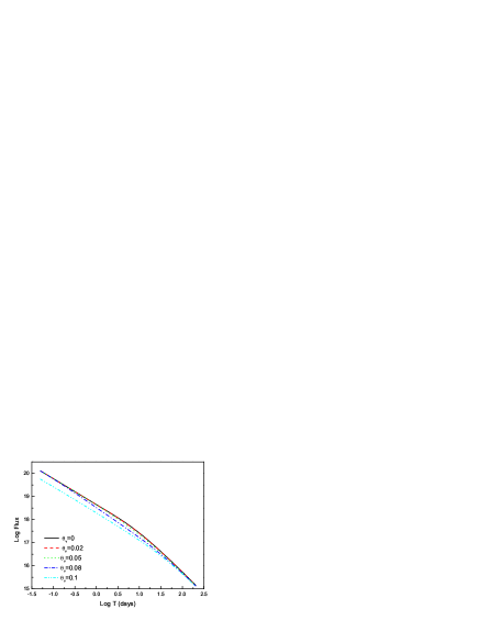
For uniform jet, the energy per unit solid angle $\epsilon$ is independent of $\theta$, $\phi$, we take $\epsilon_{54}=1$. Then using equations (2) and (9), we can calculate the jet emission for different viewing angles. Fig.1 gives our numerical results. From Fig.1 we see that the afterglow light curves for different viewing angles are somewhat different: in general, there are two breaks in the light curve, the first one corresponds to the time at which $\gamma\sim(\theta_{j}-\theta_{v})^{-1}$, and the second one corresponds to the time when $\gamma\sim(\theta_{j}+\theta_{v})^{-1}$. This is quite different from the previous results, which think there is one break occurred at $\gamma\sim\theta_{j}^{-1}$.

Figure 1: The afterglow light curves from uniform jet for various viewing angles.

4 Emission from non-uniform jet

Uniform jet is only a special case, in general we expect the jet is non-uniform, for instance, the collapsar model predicted that the jet is non-uniform, within which the energy per unit solid angle decreases away from the jet axis (e.g. MacFadyen et al. 2001). Here we suppose the energy per unit solid angle has the form

$$\epsilon=\left\{\begin{array}[]{ll}\epsilon_{0}&\;\;{\rm for}\;\;\;\;\;0\leq\theta\leq\theta_{c}\\ \epsilon_{0}(\frac{\theta}{\theta_{c}})^{-k}&\;\;{\rm for}\;\;\;\;\;\theta_{c}\leq\theta\leq\theta_{j}\end{array}\right.$$ (10)

where $\theta_{c}$ is introduced to avoid a divergence at $\theta=0$. For arbitrary viewing angle $\theta_{v}$, the situation is very complicated, so first we consider the case $\theta_{v}=0$, since this can give an analytical analysis.

In the case of $\theta_{v}=0$, we have $\mu=\cos\theta$. It should be noted that there is an interesting phenomenon, the values of $\gamma\theta$ increase with the angle $\theta$, i.e. there is a characteristic angle $\theta_{\star}$, at which the value $\gamma_{\star}\theta_{\star}=1$, when $\theta<\theta_{\star}$ the value $\gamma\theta<1$, and when $\theta>\theta_{\star}$ the value $\gamma\theta>1$. It is obvious that the main contribution of emission comes from the region $\theta\leq\theta_{\star}$, so $\theta_{\star}$ is an important quantity. It can be shown that when $T\leq T_{1}\equiv 1.7(\frac{\epsilon_{0,54}}{n_{1}})^{1/3}(\frac{\theta_{c}}{0.02})^{8/3}$ hours, the value $\theta_{\star}=10^{-1.27}(\frac{\epsilon_{0,54}}{n_{1}})^{-1/8}T_{day}^{3/8}\leq\theta_{c}$, and when $T\leq T_{2}\equiv 5.2\times(0.2)^{k/3}(\frac{\epsilon_{0,54}}{n_{1}})^{1/3}(\frac{\theta_{c}}{0.02})^{k/3}(\frac{\theta_{j}}{0.1})^{(8-k)/3}$ days, the value $\theta_{\star}=10^{-1.27\times 8/(8-k)}(\frac{\epsilon_{0,54}}{n_{1}})^{-1/(8-k)}\theta_{c}^{-k/(8-k)}T_{day}^{3/(8-k)}\leq\theta_{j}$.

Taking equation (5) and the approximate expression $1-\beta\mu\simeq(2\gamma^{2})^{-1}$ for $\theta<\theta_{\star}$, or $1-\beta\mu\simeq\frac{1}{2}\theta^{2}$ for $\theta>\theta_{\star}$, we can get the analytical results: (1) when $T\leq T_{1}$, the observed flux $F_{\nu}\propto T^{-3(p-1)/4}$; (2) when $T_{1}\leq T\leq T_{2}$, the flux $F_{\nu}\propto T^{-\frac{3(2p+k-2)}{8-k}}$ for $k<\frac{8}{p+4}$, or $F_{\nu}\propto T^{-3p/4}$ for $k>\frac{8}{p+4}$; (3) when $T>T_{2}$, the flux $F_{\nu}\propto T^{-3p/4}$. From this result we see that, for smaller value of $k$, the transition of the afterglow light curve index from $-\frac{3(p-1)}{4}$ to $-\frac{3p}{4}$ is gradual and smooth with a timescale of about $T_{2}$, while for larger values of $k$, the transition is rapid with a timescale of about $T_{1}$.

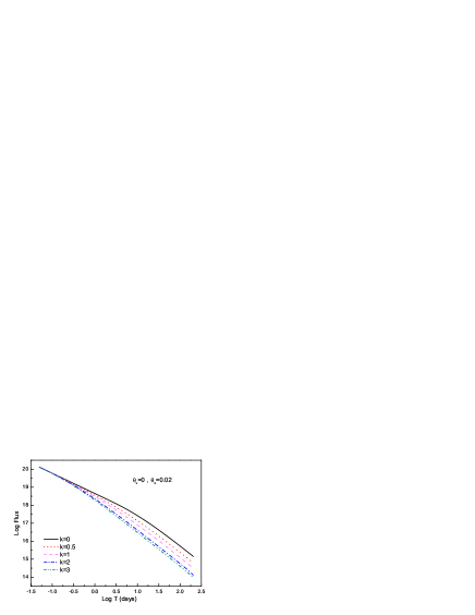
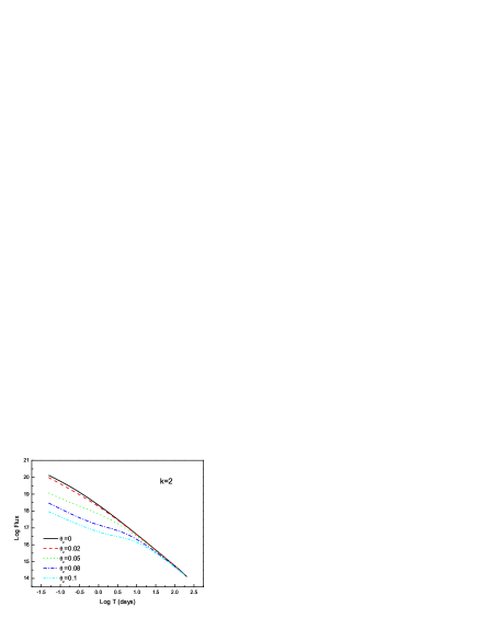
In order to verify the above results, we also make a numerical calculation for the case $\theta_{v}=0$. Fig.2 gives our results. It is obvious that the numerical results are consistent with the analytical results, for larger value of $k$, the steepening of the light curve is more rapidly. We suggest this may explain some afterglow light curves which decay rapidly and have no breaks, since for larger value of $k$ the transition time ($\sim T_{1}$) is earlier than our first observation time.

However, it should be noted that the appearance of the early break in the light curve (corresponding to the time when $\gamma\sim\theta_{c}^{-1}$) is due to the assumed energy distribution function (equation (10)), and the sharpness of this break is primarily dependent on the discontinuity in slope of $\epsilon$ for the idealized model of equation (10) at $\theta=\theta_{c}$. It is obvious that for a realistic energy distribution, the transition of $\epsilon$ from roughly constant for $\theta<\theta_{c}$ to $\epsilon\propto\theta^{-k}$ for $\theta>\theta_{c}$ should be smooth. Therefore this break may be washed out by a realistic energy distribution.

Figure 2: The afterglow light curves from non-uniform jet for the case $\theta_{v}=0$.

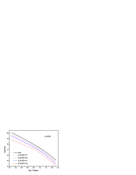
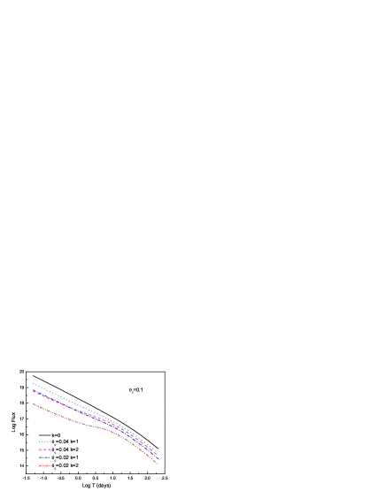
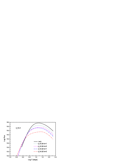
For the general case $\theta_{v}\neq 0$, we calculate the afterglow light curves numerically using equations (2), (9) and (10), the results are given in Fig.3 - Fig.6. From these figures we see that the afterglow light curves are dependent on the values of $\theta_{v}$, $\theta_{c}$ and $k$. When $\theta_{v}$ is near $\theta_{c}$ and $k$ is small, then the light curve is similar to the case of $\theta_{v}=0$, except the flux is somewhat lower. However, if the viewing angle $\theta_{v}$ is larger than $\theta_{c}$ and $k$ is not very small, then there will be a prominent flattening in the afterglow light curve, which is quite different from the case of uniform jet, and after the flattening a very sharp break will be occurred around the time $\gamma\sim(\theta_{v}+\theta_{c})^{-1}$. If the viewing angle $\theta_{v}$ is larger than the jet half-opening angle $\theta_{j}$, then the flux will first increase with time until the Lorentz factor is about $\gamma\sim(\theta_{v}-\theta_{j})^{-1}$, thereafter the flux begin to decay with time.

Figure 3: The afterglow light curves from non-uniform jet for the case $\theta_{v}=0.06$.

Figure 4: The afterglow light curves from non-uniform jet for the case $\theta_{v}=0.1$.

Figure 5: The afterglow light curves from non-uniform jet for the case $\theta_{v}=0.2$.

Figure 6: The afterglow light curves from non-uniform jet ($k=2$) for different viewing angles.

5 Discussion and conclusion

In this paper we calculate the GRB afterglow light curves from relativistic jets in more details, assuming that the jet may be uniform or non-uniform, and the observer locate at arbitrary angle with respect to the jet axis. We have shown that there are several distinct features of our jet emission compared with previous jet model.

In previous analysis, it is generally assumed that the jet is uniform and the line-of-sight is just along the jet axis, in this case the afterglow light curves have a break at the time $\gamma\sim\theta_{j}^{-1}$. However, if the viewing angle $\theta_{v}\neq 0$, we have shown that there should be two breaks in the light curve, the first one corresponds to the time at which $\gamma\sim(\theta_{j}-\theta_{v})^{-1}$, and the second one corresponds to the time when $\gamma\sim(\theta_{j}+\theta_{v})^{-1}$, although these transitions are very smoothly.

If the jet is not uniform, within which the energy distribution is given by eq.(10), then the calculation is more complicated. In the case of $\theta_{v}=0$, we can give an analytical result, for $k<8/(p+4)$(where $p$ is the spectral index of electron energy distribution) there should be two breaks in the light curve correspond to $\gamma\sim\theta_{c}^{-1}$ and $\gamma\sim\theta_{j}^{-1}$ respectively, while for $k>8/(p+4)$ there should be only one break corresponds to $\gamma\sim\theta_{c}^{-1}$, after that the flux decays as $F_{\nu}\propto T^{-3p/4}$. We argue that this may explain some rapidly fading afterglows whose light curves have no breaks, since the time $T_{1}$, at which $\gamma\sim\theta_{c}^{-1}$, is usually earlier than our first observation time.

If the jet is non-uniform and the viewing angle $\theta_{v}\neq 0$, only numerical results can be given. We have shown that in this case the shape of afterglow light curve is dependent on the values of $\theta_{v}$, $\theta_{c}$ and $k$. When $\theta_{v}$ is near $\theta_{c}$ and $k$ is small, then the light curve is similar to the case of $\theta_{v}=0$, except the flux is somewhat lower. However, if the viewing angle $\theta_{v}$ is larger than $\theta_{c}$ and $k$ is not small, then there will be a prominent flattening in the afterglow light curve, which is quite different from the case of uniform jet, and after the flattening a very sharp break will be occurred around the time $\gamma\sim(\theta_{v}+\theta_{c})^{-1}$. We think this is a main difference between the uniform and non-uniform jet, and we can identify whether the jet is uniform or not by this feature.

It is not very difficult to understand why sometimes there is a flattening in the light curve. It is well known that, for a relativistic blast wave with Lorentz factor $\Gamma\gg 1$, the observer can only observe a solid angle around $\theta_{v}$ with a half opening angle of order $\Gamma^{-1}$, the contribution from other components can be neglected, so when the blast wave decelerates, the observer can see larger components. For the case of non-uniform jet and $\theta_{v}>\theta_{c}$, the energy at $\theta=\theta_{v}$ is much smaller than that of smaller $\theta$, so when $\Gamma$ decreases, the observer can observe more region with larger energy (smaller $\theta$), so there will be a flattening in the light curve.

We would point out that, in our calculation we have neglected the sideways expansion of the jet since this process is too complicated. However, we know that, in fact this process is an important issue in determining the shape of a light curve, since it will likely significantly change the shape of the light curve for both the uniform and non-uniform jets. So we suggest that for a more realistic calculation the sideways expansion should be taken into account.