Quintessence with a constant equation of state in hyperbolic universes

Abstract

Quintessence models leading to a constant equation of state are studied in hyperbolic universes. General properties of the quintessence potentials $V(\phi)$ are discussed, and for some special cases also the exact analytic expressions for these potentials are derived. It is shown that the observed angular power spectrum of the cosmic microwave background (CMB) is in excellent agreement with some of the quintessence models even in cases with negative curvature. It is emphasized that due to a $(w_{\phi},\Omega_{\phi},\Omega_{\hbox{\scriptsize c}})$-degeneracy a universe with negative spatial curvature cannot be excluded.

I Introduction

The recent observations of the anisotropy of the cosmic microwave background (CMB) Netterfield_et_al_2001 ; Lee_et_al_2001 ; Halverson_et_al_2001 together with the power spectrum of the large scale structure (LSS) Peacock_Dodds_1994 ; Hamilton_Tegmark_Padmanabhan_2000 ; Percival_et_al_2001 ; Efstathiou_2dF_team_2002 , and the magnitude-redshift relation of the supernovae Ia Hamuy_et_al_1996 ; Riess_et_al_1998 ; Perlmutter_et_al_1999 give strong evidence that the present mean energy density $\varepsilon_{\hbox{\scriptsize tot}}$ of the universe consists not only of radiation, baryonic and cold dark matter, but also of a dominant component with negative pressure which nowadays is called dark energy. An obvious candidate for this new energy is Einstein’s cosmological constant $\Lambda$ with a corresponding constant energy density $\varepsilon_{\Lambda}=\Lambda c^{4}/(8\pi G)$ and negative pressure $p_{\Lambda}=-\varepsilon_{\Lambda}$, assuming a positive cosmological constant. The associated cosmological models are known as $\Lambda$CDM models.

An alternative explanation for the missing energy is quintessence, where the dark energy density is identified with the energy density $\varepsilon_{\phi}$ (associated with a negative pressure $p_{\phi}$) arising from a scalar (quintessence) field $\phi$ (see Peebles_Ratra_2002 for a recent review). Quintessence can be considered as a natural generalization of the cosmological constant to the case of a time-dependent $\Lambda(t)$ with an associated time-dependent pressure.

Many cosmologists seem to accept as established that the universe is flat corresponding to $k=0$ and $\Omega_{\hbox{\scriptsize tot}}:=\varepsilon_{\hbox{\scriptsize tot}}/\varepsilon_{\hbox{\scriptsize crit}}=1$. Here we address the question: do the recent observations really establish that our universe is spatially flat? It is demonstrated that present data are consistent with certain quintessence models possessing a constant equation of state in a hyperbolic universe, i. e. with negative spatial curvature, $k=-1$, corresponding to $\Omega_{\hbox{\scriptsize tot}}<1$. Our result is the consequence of the important observation that there exists a degeneracy in the space of the relevant cosmological parameters $(w_{\phi},\Omega_{\phi},\Omega_{\hbox{\scriptsize c}})$ which are introduced below.

Our background model is the standard cosmological model based on a Friedmann–Lemaître universe with the Robertson-Walker metric

$$ds^{2}\;=\;a^{2}(\eta)\,\left(d\eta^{2}-\gamma_{ij}dx^{i}dx^{j}\right)\hskip 10.0pt,$$ (1)

where $\gamma_{ij}$ denotes the spatial hyperbolic metric, and $a(\eta)$ is the cosmic scale factor as a function of conformal time $\eta$. Then the Friedmann equation reads $(a^{\prime}:=da/d\eta,c=1)$

$$H^{2}:=\left(\frac{a^{\prime}}{a^{2}}\right)^{2}\;=\;\frac{8\pi G}{3}\varepsilon_{\hbox{\scriptsize tot}}+\frac{1}{a^{2}}\hskip 10.0pt,$$ (2)

where $H=H(\eta)$ is the Hubble parameter, and the last term in Eq. (2) is the curvature term for $k=-1$. Furthermore, $\varepsilon_{\hbox{\scriptsize tot}}=\varepsilon_{\hbox{\scriptsize r}}+\varepsilon_{\hbox{\scriptsize m}}+\varepsilon_{\phi}$, where $\varepsilon_{\hbox{\scriptsize r}}$ denotes the energy density of “radiation”, i. e. of the relativistic components according to photons and three massless neutrinos; $\varepsilon_{\hbox{\scriptsize m}}=\varepsilon_{\hbox{\scriptsize b}}+\varepsilon_{\hbox{\scriptsize cdm}}$ is the energy density of non-relativistic “matter” consisting of baryonic matter, $\varepsilon_{\hbox{\scriptsize b}}$, and cold dark matter, $\varepsilon_{\hbox{\scriptsize cdm}}$, and $\varepsilon_{\phi}$ is the energy density of the dark energy due to the quintessence field $\phi$. (In Sect. V.3, we will also include the energy density due to a cosmological constant.) For our later discussions of the time-dependence $\varepsilon_{\hbox{\scriptsize x}}=\varepsilon_{\hbox{\scriptsize x}}(\eta)$ of the various energy components $({\hbox{x}}={\hbox{r}},{\hbox{m}},\phi)$, it is important to notice that the initial conditions to be imposed on the Friedmann equation (2) are in the case of negative curvature uniquely given by $a(0)=0$ and $a^{\prime}(0)=\Omega_{\hbox{\scriptsize r}}^{1/2}(1-\Omega_{\hbox{\scriptsize tot}})^{-1}H_{0}^{-1}$ with $H_{0}=H(\eta_{0})$ being the Hubble constant. Here and in the following, we use the dimensionless density parameters $\Omega_{\hbox{\scriptsize x}}(\eta):=\varepsilon_{\hbox{\scriptsize x}}(\eta)/\varepsilon_{\hbox{\scriptsize crit}}(\eta)$ with $\varepsilon_{\hbox{\scriptsize crit}}(\eta)=3H^{2}/(8\pi G)$ and $\Omega_{\hbox{\scriptsize x}}:=\Omega_{\hbox{\scriptsize x}}(\eta_{0})$ denoting their present values.

In quintessence models, the energy density $\varepsilon_{\phi}(\eta)$ and the pressure $p_{\phi}(\eta)$ of the dark energy are determined by the quintessence potential $V(\phi)$

$$\varepsilon_{\phi}\;=\;\frac{1}{2a^{2}}\,{\phi^{\prime}}^{2}+V(\phi)\hskip 10.0pt,\hskip 10.0ptp_{\phi}\;=\;\frac{1}{2a^{2}}\,{\phi^{\prime}}^{2}-V(\phi)\hskip 10.0pt,$$ (3)

or equivalently by the equation of state

$$w_{\phi}(\eta)\;=\;\frac{p_{\phi}(\eta)}{\varepsilon_{\phi}(\eta)}\hskip 10.0pt.$$ (4)

The equation of motion of the real, scalar field $\phi(\eta)$ is

$$\phi^{\prime\prime}\,+\,2\frac{a^{\prime}}{a}\phi^{\prime}\,+\,a^{2}\frac{\partial V(\phi)}{\partial\phi}\;=\;0\hskip 10.0pt,$$ (5)

where it is assumed that $\phi$ couples to matter only through gravitation. The various energy densities are constrained by the continuity equation

$$\varepsilon_{\hbox{\scriptsize x}}^{\prime}(\eta)\,+\,3(1+w_{\hbox{\scriptsize x}}(\eta))\,\frac{a^{\prime}}{a}\,\varepsilon_{\hbox{\scriptsize x}}(\eta)\;=\;0\hskip 10.0pt,$$ (6)

with the constant equation of state $w_{\hbox{\scriptsize r}}=\frac{1}{3}$, $w_{\hbox{\scriptsize m}}=0$ for $\hbox{x}=\hbox{r},\hbox{m}$ and $w_{\phi}(\eta)$ for $\hbox{x}=\phi$. It is worthwhile to remark that the quintessence field $\phi$ may be regarded as a real physical field, or simply as a device for modeling more general cosmic fluids with negative pressure.

Obviously, there are two complementary approaches:

• Given $V(\phi)$ compute $w_{\phi}(\eta)$,

• Given $w_{\phi}(\eta)$ compute $V(\phi)$,

and then make predictions for or compare with cosmological observations. Among the various potentials studied in the literature (see, e. g. Peebles_Ratra_2002 ; Brax_Martin_Riazuelo_2000 and references therein), we mention only the inverse power-law potential

$$V(\phi)\;=\;\frac{A}{(B\phi)^{\gamma}}\hskip 10.0pt,\hskip 10.0pt\gamma>0\hskip 10.0pt,$$ (7)

and the exponential potential

$$V(\phi)\;=\;A\,\exp(-B\phi)\hskip 10.0pt,\hskip 10.0ptB>0\hskip 10.0pt.$$ (8)

The potentials (7) and (8) can be derived Ratra_Peebles_1988 (see also Sect. III), if one requires a constant $w_{\phi}$ during a given evolution stage of the universe: in the radiation-dominated epoch one obtains the inverse power-law potential (7), whereas in the quintessence-dominated epoch one requires $w_{\phi}=\hbox{const.}\leq-1/3$ and then obtains the exponential potential (8).

In the following, we concentrate our attention on approach b), where one specifies the equation of state $w_{\phi}$ rather than the potential $V(\phi)$. In order to generalize the standard cosmological models like $\Lambda$CDM models with as few as possible additional degrees of freedom, $w_{\phi}$ will be chosen as constant (as studied for flat universes in, e. g., Caldwell_Dave_Steinhardt_1998 ; Wang_Steinhardt_1998 ) This contrasts to approach a), where a whole function, i. e. the potential $V(\phi)$, increases the freedom of the model enormously. Furthermore, since in the standard cosmological theories $w_{\hbox{\scriptsize x}}$ is constant for the various energy components, one can also consider a constant $w_{\phi}$ for the dark energy component as the most “natural” generalization. It turns out that the values $w_{\phi}=-1/3,-2/3$ play a special role and constitute a kind of new “exceptional phases” in addition to the standard phases characterized by $w_{\hbox{\scriptsize x}}=\{1/3,0,-1\}$ for $\hbox{x}=\{\hbox{r},\hbox{m},\Lambda\}$. Such equations of state occur in models based on topological defects where $w=-1/3$ corresponds to a network of frustrated cosmic strings Vilenkin_1984 ; Spergel_Pen_1997 and $w=-2/3$ to domain walls Durrer_Kunz_Melchiorri_2002 ; Gangui_2001 .

One purpose of this paper is to derive the potential $V(\phi)$ for the two special equations of state $w_{\phi}=-1/3,-2/3$. The restriction to a constant equation of state arises from the absence of well motivated dark energy models being based on fundamental physics. This restriction should not only be considered as a prejudice but also as an approximation to time-variable equations of state when one attempts to describe cosmological observations. Models with a non-constant equation of state lead to nearly the same CMB anisotropy as corresponding models with an effective (constant) equation of state where $w_{\phi}(\eta)$ is appropriately $\Omega_{\phi}$-averaged Doran_Lilley_Schwindt_Wetterich_2001 ; Doran_Lilley_2002 . As argued in Doran_Lilley_Schwindt_Wetterich_2001 , the location of the acoustic peaks is mainly determined by $\Omega_{\phi}(\eta_{0})$, the $\Omega_{\phi}$-weighted average of $w_{\phi}(\eta)$ averaged until the present time, as well as by the average of $\Omega_{\phi}(\eta)$ until recombination. The latter is negligible for negative $w_{\phi}(\eta)$, i. e. for non-tracker field models, since around $z_{\hbox{\scriptsize sls}}\simeq 1100$ the energy density of the quintessence component is then subdominant compared to that of the background component. Thus $\Omega_{\phi}(\eta_{0})$ and the $\Omega_{\phi}$-weighted average of $w_{\phi}(\eta)$ suffice to approximately describe the peak structure. Since the dark energy dominates only recently, the $\Omega_{\phi}$-weighted average leads to an averaging over the recent history. Therefore, the anisotropy of the CMB is not well suited to probe the time-dependence of the equation of state $w_{\phi}(\eta)$. The main properties of the anisotropy are then determined by the angular-diameter distance $d_{A}$ to the surface of last scattering (see, e. g., Cornish_2000 ). A further dependence of the CMB anisotropy on the dark energy arises through the late-time integrated Sachs-Wolfe effect which contributes mostly to low multipoles in the angular power spectrum. Because of the cosmic variance and a possible contribution of gravity waves, it is difficult to extract information on a time-varying equation of state Corasaniti_Bassett_Ungarelli_Copeland_2002 . On the other hand, in classical cosmological tests based on the luminosity distance, a dark energy component contributes appreciably only for redshifts $0.2\lesssim z\lesssim 2$ Huterer_Turner_2001 since for higher redshifts the contribution to the total energy density is too minute (see also Eq. (51)). Here the difficulties are caused by the luminosity distance which depends on $w_{\phi}(\eta)$ through a multiple-integral which smears out the information on the time-dependence of $w_{\phi}(\eta)$ Maor_Brustein_Steinhardt_2001 . Thus, with the exception of tracker fields, it is very difficult to observe a time-dependence of $w_{\phi}(\eta)$ and therefore one can restrict the discussion to a constant equation of state.

Quintessence models with a constant equation of state differ from a cosmological constant with $w_{\Lambda}=-1$ only in the value of the constant $w_{\phi}\neq-1$. If the observations are too close to $w_{\phi}\simeq w_{\Lambda}$, then quintessence models might be superseded by the long-known cosmological constant, i. e. by the vacuum energy. Assuming flat universes, the current bound is, e. g., $w_{\phi}<-0.85$ at 68% C.L. Bean_Melchiorri_2002 or even $w_{\phi}<-0.93$ at $2\sigma$ Corasaniti_Copeland_2002 . The caveat is, as we shall show in Sect. VI, the assumed flatness. Such a value so close to the cosmological constant has, however, problems to account for the observed number of giant arcs in galaxy clusters. For a flat $\Lambda$CDM model with $\Omega_{\hbox{\scriptsize m}}=0.3$, the number of arcs is one order of magnitude too low. To obtain the right order, one either needs a low-density open model with $\Omega_{\hbox{\scriptsize m}}=0.3$ or a flat model where the vacuum energy is replaced by a dark energy component with $w_{\phi}\simeq-0.6$ Bartelmann_Meneghetti_Perrotta_Baccigalupi_Moscardini_2002 . A further variant, not discussed in Bartelmann_Meneghetti_Perrotta_Baccigalupi_Moscardini_2002 , would be an open model with dark energy which should also produce enough strong lensing to obtain a large number of arcs. In addition, too few lensed pairs with wide angular separation are observed in comparison with the prediction of a flat $\Lambda$CDM-model Sarbu_Rusin_Ma_2001 . These strong lensing observations point towards a universe with negative curvature.

II General Formula for the Quintessence Potential

In the following, general properties of quintessence models having a constant equation of state $w_{\phi}$ with $w_{\phi}\in[-1,-1/3]$ and for a universe with negative curvature, i. e. $\Omega_{\hbox{\scriptsize tot}}<1$, will be discussed. Especially, we discuss the properties of the potential $V(\phi)$ which belongs to a given $w_{\phi}$. Without loss of generality, we may assume $\phi(\eta)\geq 0$ with the initial value $\phi_{\hbox{\scriptsize in}}=\phi(0)=0$. It then will turn out that the potential $V(\phi)$ is uniquely determined.

Our starting point are the simple relations

$$V(\phi)\;=\;\frac{1}{2}\left(\varepsilon_{\phi}-p_{\phi}\right)\;=\;\frac{1-w_{\phi}}{2}\,\varepsilon_{\phi}\hskip 10.0pt,$$ (9)

$${\phi^{\prime}}^{2}\;=\;a^{2}\,\left(\varepsilon_{\phi}+p_{\phi}\right)\;=\;(1+w_{\phi})\,a^{2}\,\varepsilon_{\phi}\hskip 10.0pt,$$ (10)

which directly follow from Eqs. (3) and (4). Since $w_{\phi}$ is constant, we obtain the following solution for $\varepsilon_{\phi}$ from the continuity equation (6)

$$\varepsilon_{\phi}(\eta)\;=\;\varepsilon_{\phi}(\eta_{0})\,\left(\frac{a_{0}}{a(\eta)}\right)^{3(1+w_{\phi})}\hskip 10.0pt,$$ (11)

where $a_{0}=a(\eta_{0})=H_{0}^{-1}(1-\Omega_{\hbox{\scriptsize tot}})^{-1/2}$ is the scale factor of the present epoch. Inserting (11) into (9), we arrive at the following exact expression for the potential $V(\phi(\eta))$ parameterized in terms of the scale factor $a(\eta)$

$$V(\phi(\eta))\;=\;\tilde{V}_{0}\,\left(\frac{a_{0}}{a(\eta)}\right)^{3(1+w_{\phi})}\hskip 10.0pt,$$ (12)

where the “potential strength” $\tilde{V}_{0}=V(\phi(\eta_{0}))$ is given by

$$\tilde{V}_{0}\;=\;\frac{1-w_{\phi}}{2}\,\Omega_{\phi}\,\varepsilon_{\hbox{\scriptsize crit}}\hskip 10.0pt,$$ (13)

with $\Omega_{\phi}=\Omega_{\phi}(\eta_{0})=\varepsilon_{\phi}(\eta_{0})/\varepsilon_{\hbox{\scriptsize crit}}$ and $\varepsilon_{\hbox{\scriptsize crit}}=\varepsilon_{\hbox{\scriptsize crit}}(\eta_{0})=3H_{0}^{2}/(8\pi G)$. Although Eq. (12) does not yet express $V(\phi)$ as a function of $\phi$, several important conclusions can already be drawn from Eqs. (12) and (13):

• $V(\phi)$ is always positive, $V(\phi)\geq 0$,

• $V(\phi(\eta))$ diverges for $w_{\phi}=\text{const.}>-1$ like

  $$V(\phi(\eta))\;=\;O\left(\frac{1}{\eta^{3(1+w_{\phi})}}\right)$$ (14)

  in the radiation-dominated epoch, $\eta\to 0$, since $a(\eta)=O(\eta)$ in this limit,

• $V(\phi(\eta))$ decreases monotonically with increasing $\eta$, since $a(\eta)$ increases monotonically,

• the order of magnitude of the potential strength $\tilde{V}_{0}$, Eq. (13), is determined by the “small” energy density $\varepsilon_{\hbox{\scriptsize crit}}$.

The divergent behavior (14) for $w_{\phi}>-1$ implies that $V(\phi(\eta))$ does not possess a Taylor expansion at $\eta=0$, i. e. at $\phi_{\hbox{\scriptsize in}}$. This in turn is tightly connected with the fact that assuming a Taylor expansion at $\phi=\phi_{\hbox{\scriptsize in}}$ necessarily implies a time-varying $w_{\phi}$ with $w_{\phi}(0)=-1$. (A proof will be given in Sect. III.)

As a side-remark, notice that Eqs. (12) and (13) are consistent with the standard cosmological constant, since $w_{\phi}=-1$ yields $V(\phi)=\tilde{V}_{0}=\varepsilon_{\phi}=\text{const.}$ for all $\eta\geq 0$.

In order to determine $V(\phi)$ as a function of $\phi$, we must replace $a(\eta)$ in Eq. (12) by $A(\phi):=a(\eta(\phi))$, where $\eta(\phi)$ is the inverse of $\phi(\eta)$. The function $A(\phi)$ can by computed as follows. Combining Eqs. (10) and (11) yields

$$\phi^{\prime}(\eta)\;=\;\alpha\,[a(\eta)]^{\delta}$$ (15)

with $\alpha:=[(1+w_{\phi})\Omega_{\phi}a_{0}^{3(1+w_{\phi})}\,\varepsilon_{\hbox{\scriptsize crit}}]^{1/2}$ and $\delta:=-\frac{1}{2}(1+3w_{\phi})$. Here we have chosen the positive square root of Eq. (10), since with $\phi(0)=0$ and $\phi(\eta)\geq 0$, the general properties i)–iii) of the potential lead to $\phi^{\prime}(\eta)\geq 0$. (Actually, Eq. (15) implies $\phi^{\prime}(\eta)\to 0$ for $\eta\to 0$ and $-1<w_{\phi}<-\frac{1}{3}$.) Furthermore, we have

$$\phi^{\prime}(\eta)\;=\;\frac{d\phi(\eta(a))}{da}\,a^{\prime}\;=\;\frac{d\phi}{dA}\,\sqrt{f(A)}\hskip 10.0pt,$$ (16)

where the function $f(a)$ is defined by rewriting the Friedmann equation (2) as ${a^{\prime}}^{2}=f(a)$ with

$$f(a) := \frac{8\pi G}{3}\,\varepsilon_{\hbox{\scriptsize tot}}(\eta)\,a^{4}+a^{2}$$ (17)

$$= H_{0}^{2}\,\sum_{\hbox{\scriptsize x}=\hbox{\scriptsize r},\hbox{\scriptsize m},\phi,\hbox{\scriptsize c}}\Omega_{\hbox{\scriptsize x}}a_{0}^{3(1+w_{\hbox{\scriptsize x}})}\,a^{1-3w_{\hbox{\scriptsize x}}}\hskip 10.0pt.$$

In the last expression, we have inserted the solutions of the continuity equation (6) for the various energy components $\hbox{x}=\{\hbox{r},\hbox{m},\phi\}$ and, furthermore, have introduced the dimensionless curvature parameter $\Omega_{\hbox{\scriptsize c}}:=(H_{0}^{2}a_{0}^{2})^{-1}=1-\Omega_{\hbox{\scriptsize tot}}>0$ with the corresponding equation of state $w_{\hbox{\scriptsize c}}=-\frac{1}{3}$. Combining Eqs. (15) and (16) gives

$$d\phi\;=\;\alpha\,\frac{A^{\delta}}{\sqrt{f(A)}}\,dA\hskip 10.0pt,$$ (18)

which yields by integration

$$\phi\;=\;\alpha\,\int_{0}^{A(\phi)}\frac{A^{\delta}}{\sqrt{f(A)}}\,dA\hskip 10.0pt.$$ (19)

Since $A(\phi)=a(\eta(\phi))$ tends to zero in the limit $\eta\to 0$, the integral relation (19) is consistent with our initial condition $\phi(\eta)\to 0$ in this limit. Eq. (19) determines the cosmic scale factor $A$ as a function of the quintessence field $\phi$, i. e. as the inverse function of the function defined by the integral in Eq. (19). Inserting the solution $A(\phi)$ of (19) into Eq. (12), leads to our general formula

$$V(\phi)\;=\;\tilde{V}_{0}\,\left(\frac{a_{0}}{A(\phi)}\right)^{3(1+w_{\phi})}$$ (20)

for the quintessence potential.

It is convenient to use the dimensionless variable $y:=\frac{A}{a_{0}}=\frac{1}{z+1}$ as an integration variable in (19). Defining the dimensionless function

$$g(y)\;:=\;\sum_{\hbox{\scriptsize x}=\hbox{\scriptsize r},\hbox{\scriptsize m},\phi,\hbox{\scriptsize c}}\Omega_{\hbox{\scriptsize x}}\,y^{1-3w_{\hbox{\scriptsize x}}}\hskip 10.0pt,$$ (21)

we have $f(A)=f(a_{0}y)=H_{0}^{2}a_{0}^{4}g(y)$, and Eq. (19) takes the final form

$$B_{0}\,\phi\;=\;\int_{0}^{A(\phi)/a_{0}}\frac{y^{-\frac{3}{2}(w_{\phi}+\frac{1}{3})}}{\sqrt{g(y)}}\,dy$$ (22)

with

$$B_{0}\;:=\;\frac{1}{m_{P}}\,\sqrt{\frac{8\pi}{3(1+w_{\phi})\Omega_{\phi}}}\hskip 10.0pt.$$ (23)

(Here $m_{P}:=G^{-1/2}$ denotes the Planck mass, $\hbar=1$.) Note that the combination $B_{0}\phi$ is dimensionless as required by the right-hand side of (22).

Before we come to a discussion of the general properties of the potential (20), we have to check whether the solution (22) for $\phi$ together with the potential (20) solves the equation of motion (5), which until now has not been used in our derivation. For this purpose, it is useful to express the time-dependence of the various terms in (5) by $a(\eta)$. Using $\phi^{\prime\prime}=\frac{d\phi^{\prime}}{da}a^{\prime}=\frac{d\phi^{\prime}}{da}\sqrt{f(a)}$ and Eq. (15), we obtain

$$\phi^{\prime\prime}\;=\;-\,\frac{\alpha\sqrt{f(a)}}{a^{\frac{3}{2}(1+w_{\phi})}}\;\frac{1+3w_{\phi}}{2}\hskip 10.0pt.$$ (24)

Furthermore, with $\frac{\partial V}{\partial\phi}=\frac{\partial V}{\partial A}\frac{dA}{d\phi}$ and Eqs. (18) and (20) we derive

$$a^{2}\,\frac{\partial V}{\partial\phi}\;=\;-\,\frac{\alpha\sqrt{f(a)}}{a^{\frac{3}{2}(1+w_{\phi})}}\,\beta$$ (25)

with $\beta:=3(1+w_{\phi})\tilde{V}_{0}a_{0}^{3(1+w_{\phi})}/\alpha^{2}=\frac{3}{2}(1-w_{\phi})$. Thus, we obtain

$$\phi^{\prime\prime}+2\frac{a^{\prime}}{a}\phi^{\prime}+a^{2}\frac{\partial V}{\partial\phi}\;=\;$$

$$= -\,\frac{\alpha\sqrt{f(a)}}{a^{\frac{3}{2}(1+w_{\phi})}}\,\frac{1+3w_{\phi}}{2}\,+\,2\frac{\sqrt{f(a)}}{a}\,\frac{\alpha}{a^{\frac{1+3w_{\phi}}{2}}}$$

$$\hskip 120.0pt-\,\frac{\alpha\sqrt{f(a)}}{a^{\frac{3}{2}(1+w_{\phi})}}\,\beta$$

$$= -\,\frac{\alpha\sqrt{f(a)}}{a^{\frac{3}{2}(1+w_{\phi})}}\,\left[\frac{1+3w_{\phi}}{2}-2+\beta\right]\;\equiv\;0\hskip 10.0pt,$$

which proves that the equation of motion is satisfied, since the square bracket in the last expression is identically zero.

III General Properties of the Quintessence Potential

For arbitrary constant values of $w_{\phi}\in(-1,-\frac{1}{3})$, it is not possible to obtain from Eq. (22) an explicit analytic expression for $A(\phi)$, and thus no explicit analytic expression exists in the general case for the potential (20). (See, however, the special cases $w_{\phi}=-\frac{1}{3},-\frac{2}{3}$ which will be discussed in Sect. V.) Nevertheless, it is possible to compute the potential for all values of $w_{\phi}$ numerically, and therefore one can calculate various quantities, which then can be compared with the cosmological observations. This will be done in Sect. VI. In this Section, we discuss some general properties which can be deduced from the formulae derived in Sect. II.

In the radiation-dominated epoch, $\eta\to 0$ or $\phi\to 0$, we have $A(\phi)\to 0$, and thus Eq. (22) gives ($\delta:=-\frac{3}{2}(\frac{1}{3}+w_{\phi})\geq 0$)

$$B_{0}\,\phi = \int_{0}^{A(\phi)/a_{0}}\frac{y^{\delta}}{\sqrt{\Omega_{\hbox{\scriptsize r}}+\Omega_{\hbox{\scriptsize m}}y+O(y^{2})}}\,dy$$ (26)

$$= \frac{1}{\sqrt{\Omega_{\hbox{\scriptsize r}}}(\delta+1)}\,\left(\frac{A(\phi)}{a_{0}}\right)^{\delta+1}\,+\,\dots\hskip 10.0pt,$$

which implies

$$A(\phi)\;=\;a_{0}\left[(\delta+1)B_{0}\sqrt{\Omega_{\hbox{\scriptsize r}}}\;\right]^{\frac{1}{\delta+1}}\,\phi^{\frac{1}{\delta+1}}\,+\,\dots\hskip 3.0pt,\hskip 3.0pt\phi\to 0\hskip 3.0pt.$$ (27)

Inserting this in (20), gives for the quintessence potential

$$V(\phi)\;=\;O\left(\frac{1}{\phi^{\gamma}}\right)\hskip 10.0pt,\hskip 10.0pt\phi\to 0\hskip 10.0pt,\hskip 10.0pt\gamma\;=\;6\,\frac{1+w_{\phi}}{1-3w_{\phi}}\hskip 7.0pt.$$ (28)

For the two exceptional cases $w_{\phi}=-1/3$ and $-2/3$, one obtains from (28) $\gamma=2$ and $2/3$, respectively. (If radiation is neglected, $\Omega_{\hbox{\scriptsize r}}=0$, while keeping $\Omega_{\hbox{\scriptsize m}}\neq 0$, as it is often assumed, one instead obtains (see Eq. (26)) $\gamma=-2(1+w_{\phi})/w_{\phi}$ which yields in the case $w_{\phi}=-1/3$ the value $\gamma=4$ instead of $\gamma=2$.) Thus, the quintessence potential behaves for $\phi\to 0$ as the inverse power-law potential (7), where the power $\gamma$ is uniquely given by Eq. (28).

In the quintessence-dominated epoch, one has $a(\eta)\to\infty$ for $\eta\to\eta_{\infty}$ with $\eta_{\infty}<\infty$ for $w_{\phi}<-\frac{1}{3}$ and $\eta_{\infty}=\infty$ for $w_{\phi}=-\frac{1}{3}$. This follows immediately from the Friedmann equation $a^{\prime}=da/d\eta=\sqrt{f(a)}$, which can be integrated to give

$$\eta\;=\;\int_{0}^{a(\eta)}\frac{da}{\sqrt{f(a)}}\;=\;\sqrt{\Omega_{\hbox{\scriptsize c}}}\int_{0}^{a(\eta)/a_{0}}\frac{dy}{\sqrt{g(y)}}\hskip 10.0pt.$$ (29)

For $w_{\phi}<-\frac{1}{3}$ this yields

$$\eta_{\infty}=\sqrt{\Omega_{\hbox{\scriptsize c}}}\int_{0}^{\infty}\frac{dy}{\sqrt{\Omega_{\phi}y^{1-3w_{\phi}}+\Omega_{\hbox{\scriptsize c}}y^{2}+\Omega_{\hbox{\scriptsize m}}y+\Omega_{\hbox{\scriptsize r}}}}<\infty\,.$$ (30)

Similarly, we obtain from (22) $\phi\to\infty$ in the limit $\eta\to\eta_{\infty}$ for $w_{\phi}\leq-\frac{1}{3}$. To get the leading asymptotic behavior of $A(\phi)$ in this limit, we have to distinguish again between two cases. For $w_{\phi}=-\frac{1}{3}$, Eq. (22) yields

$$B_{0}\,\phi = \int_{0}^{A(\phi)/a_{0}}\frac{dy}{\sqrt{(\Omega_{\phi}+\Omega_{\hbox{\scriptsize c}})y^{2}+\Omega_{\hbox{\scriptsize m}}y+\Omega_{\hbox{\scriptsize r}}}}$$ (31)

$$= \frac{1}{\sqrt{\Omega_{\phi}+\Omega_{\hbox{\scriptsize c}}}}\,\ln\left(\frac{A(\phi)}{a_{0}}\right)\,+\,\dots\hskip 10.0pt,$$

whereas for $-1<w_{\phi}<-\frac{1}{3}$ on gets

$$B_{0}\,\phi = \int_{0}^{A(\phi)/a_{0}}\frac{y^{-\frac{3}{2}(w_{\phi}+\frac{1}{3})}}{\sqrt{\Omega_{\phi}y^{1-3w_{\phi}}+O(y^{2})}}\,dy$$ (32)

$$= \frac{1}{\sqrt{\Omega_{\phi}}}\,\ln\left(\frac{A(\phi)}{a_{0}}\right)\,+\,\dots\hskip 10.0pt.$$

Thus, we obtain from Eqs. (31), (32) and (23)

$$A(\phi)\;=\;O(e^{B\phi})\hskip 10.0pt,\hskip 10.0pt\phi\to\infty\hskip 10.0pt,$$ (33)

with

$$B:=\left\{\begin{matrix}&B_{0}&\sqrt{\Omega_{\phi}+\Omega_{\hbox{\scriptsize c}}}\,=\,\frac{2\sqrt{\pi}}{m_{P}}\,\sqrt{1+\frac{\Omega_{\hbox{\scriptsize c}}}{\Omega_{\phi}}}\hbox{ for }w_{\phi}=-\frac{1}{3}\\ &B_{0}&\sqrt{\Omega_{\phi}}\,=\,\frac{2\sqrt{\pi}}{m_{P}}\,\sqrt{\frac{2}{3(1+w_{\phi})}}\hbox{ for }-1<w_{\phi}<-\frac{1}{3}\end{matrix}\right.\hskip 3.0pt.$$ (34)

Inserting the asymptotic behavior (33) in (20), gives

$$V(\phi)\;=\;O\left(e^{-\mu\phi}\right)\hskip 10.0pt,\hskip 10.0pt\phi\to\infty\hskip 10.0pt,$$ (35)

with

$$\mu := 3(1+w_{\phi})B$$ (36)

$$= \frac{2\sqrt{\pi}}{m_{P}}\left\{\begin{matrix}2\sqrt{1+\frac{\Omega_{\hbox{\scriptsize c}}}{\Omega_{\phi}}}\hbox{ for }w_{\phi}=-\frac{1}{3}\\ \sqrt{6(1+w_{\phi})}\hbox{ for }-1<w_{\phi}<-\frac{1}{3}\end{matrix}\right..$$

Thus, the quintessence potential behaves for $\phi\to\infty$ as the exponential potential (8), where the exponent $\mu$ is uniquely given by (36).

We conclude that for $w_{\phi}=\hbox{const.}\leq-1/3$ and $\Omega_{\hbox{\scriptsize tot}}=1-\Omega_{\hbox{\scriptsize c}}<1$ the derived quintessence potential (20) interpolates between the inverse power-law potential (7) for $\phi\to 0$ and the exponential potential (8) for $\phi\to\infty$. There arises then the question: does there exist a closed analytic expression for $V(\phi)$ valid for all $\phi\geq 0$? In Sect. V we shall study the special cases $w_{\phi}=-\frac{1}{3},-\frac{2}{3}$ and shall show that for these cases there exist, indeed, exact analytic expressions for the potential.

Before closing this section, we would like to show that the divergent behavior (28) for $\phi\to 0$ (see also Eq. (14)), which makes it impossible to expand $V(\phi)$ at $\phi=0$ into a Taylor series, is a consequence of the assumption that the quintessence field has a constant equation of state.

Let us suppose, on the contrary, that we have a potential $V(\phi)$ which possesses a well-defined Taylor expansion at some initial field $\phi_{\hbox{\scriptsize in}}=\phi(0)$, i. e.

$$V(\phi)\;=\;v_{0}+v_{1}(\phi-\phi_{\hbox{\scriptsize in}})\,+\,O\left((\phi-\phi_{\hbox{\scriptsize in}})^{2}\right)$$ (37)

with $v_{0}:=V(\phi_{\hbox{\scriptsize in}})>0$, $v_{1}:=\frac{\partial V}{\partial\phi}(\phi_{\hbox{\scriptsize in}})\neq 0$, while $\phi(\eta)$ has at $\eta=0$ the expansion $(b\neq 0,\sigma>0)$

$$\phi(\eta)\;=\;\phi_{\hbox{\scriptsize in}}\,+\,b\,\eta^{\sigma}(1+O(\eta))\hskip 10.0pt.$$ (38)

Using the expansions (37), (38) and the well-known expansion of the scale factor in the radiation-dominated epoch, $a(\eta)=a^{\prime}(0)\,\eta+O(\eta^{2})$, it is not difficult to see that the equation of motion (5) is satisfied iff $\sigma=4$ and $b=-\frac{v_{1}}{20}{a^{\prime}}^{2}(0)$.

Now, let us consider the equation of state (4), which by means of (3) can be rewritten as

$$w_{\phi}(\eta)\;=\;-\,\frac{1-r_{\phi}(\eta)}{1+r_{\phi}(\eta)}\hskip 10.0pt,\hskip 10.0ptr_{\phi}(\eta)\;:=\;\frac{T(\eta)}{V(\phi(\eta))}\hskip 10.0pt.$$ (39)

Here $r_{\phi}$ denotes the ratio of the kinetic energy $T(\eta):={\phi^{\prime}}^{2}/(2a^{2})$ of the quintessence field to its potential energy $V$. From the above equations, one derives that $T$ vanishes like $O(\eta^{4})$, which leads to

$$r_{\phi}(\eta)\;=\;\frac{1}{50}\,\frac{v_{1}^{2}}{v_{0}}\,{a^{\prime}}^{2}(0)\,\eta^{4}\,+\,O(\eta^{5})$$ (40)

and

$$w_{\phi}(\eta)\;=\;-1\,+\,\frac{1}{25}\,\frac{v_{1}^{2}}{v_{0}}\,{a^{\prime}}^{2}(0)\,\eta^{4}\,+\,O(\eta^{5})$$ (41)

in the limit $\eta\to 0$. Thus, in such a model the quintessence component is strongly suppressed at early times and practically indistinguishable from a cosmological constant with $w_{\Lambda}=-1$. However, with increasing time $\eta$, $w_{\phi}(\eta)$ increases and therefore cannot stay constant at a value $w_{\phi}\in[-1,-\frac{1}{3}]$ for all times.

An example of a quintessence model of this type is given by the exponential potential (8) for which $\phi_{\hbox{\scriptsize in}}$ can be set to zero without loss of generality. This model has been studied in detail, e. g., in Aurich_Steiner_2002a for hyperbolic universes. Here $w_{\phi}(\eta)$ starts out at $-1$ and then approaches zero in the flat case or $-\frac{1}{3}$ in the hyperbolic case. This shows clearly, as stated already, why our assumption of a constant equation of state necessarily implies an inverse power-law divergence of $V(\phi)$ in the radiation-dominated epoch, see Eq. (28).

IV Time-Evolution of the Energy Density Parameters $\Omega_{\hbox{\scriptsize x}}(\eta)$

In this Section, we study the time-dependence of the dimensionless energy density parameters $\Omega_{\hbox{\scriptsize x}}(\eta)=\varepsilon_{\hbox{\scriptsize x}}(\eta)/\varepsilon_{\hbox{\scriptsize crit}}(\eta)$ for the various energy components $\hbox{x}=\{\hbox{r},\hbox{m},\phi\}$ as well as for $\hbox{x}=\hbox{tot}$ referring to the total energy density. From the continuity equation (6) we obtain for $\hbox{x}=\{\hbox{r},\hbox{m},\phi\}$

$$\varepsilon_{\hbox{\scriptsize x}}(\eta)\;=\;\varepsilon_{\hbox{\scriptsize x}}(\eta_{0})\,\left(\frac{a_{0}}{a(\eta)}\right)^{3(1+w_{\hbox{\scriptsize x}})}\hskip 10.0pt,$$ (42)

since all three components are assumed to possess a constant equation of state $w_{\hbox{\scriptsize x}}$. Expressing the Hubble parameter $H(\eta)$ entering $\varepsilon_{\hbox{\scriptsize crit}}(\eta)$ by the Friedmann equation (2) and using the variable $y:=\frac{a}{a_{0}}=\frac{1}{z+1}$ together with the function $g(y)$, see Eq. (21), one obtains

$$\Omega_{\hbox{\scriptsize x}}(\eta)\;=\;\frac{y^{1-3w_{\hbox{\scriptsize x}}}}{g(y)}\,\Omega_{\hbox{\scriptsize x}}\hskip 10.0pt,\hskip 10.0pt\hbox{x}=\{\hbox{r},\hbox{m},\phi\}\hskip 10.0pt.$$ (43)

The general relation (43) determines the time-evolution of the parameters $\Omega_{\hbox{\scriptsize x}}(\eta)$ in terms of their present values $\Omega_{\hbox{\scriptsize x}}=\Omega_{\hbox{\scriptsize x}}(\eta_{0})$ parameterized by the scale factor $a(\eta)$, respectively the redshift $z$. It follows immediately $\Omega_{\hbox{\scriptsize r}}(0)=1$ and $\Omega_{\hbox{\scriptsize m}}(0)=\Omega_{\phi}(0)=0$. With $\Omega_{\hbox{\scriptsize tot}}(\eta)=\sum_{\hbox{\scriptsize x}=\hbox{\scriptsize r},\hbox{\scriptsize m},\phi}\Omega_{\hbox{\scriptsize x}}(\eta)$ and Eqs. (43) and (21) one derives

$$\Omega_{\hbox{\scriptsize tot}}(\eta)\;=\;1\,-\,\frac{y^{2}}{g(y)}\,(1-\Omega_{\hbox{\scriptsize tot}})$$ (44)

satisfying $\Omega_{\hbox{\scriptsize tot}}(0)=1$. (Notice that $g(1)=\Omega_{\hbox{\scriptsize tot}}+\Omega_{\hbox{\scriptsize c}}=1$.)

To analyze the behavior of Eqs. (43) and (44) in the radiation-dominated epoch, we observe that Eq. (29) determines in the case $w_{\phi}\leq-\frac{1}{3}$ the first two terms of the scale factor $a(\eta)$ uniquely

$$y\;=\;\frac{a(\eta)}{a_{0}}\;=\;\frac{a^{\prime}(0)}{a_{0}}\left(\eta+\frac{\eta^{2}}{2\hat{\eta}}+O(\eta^{3})\right)$$ (45)

with $\hat{\eta}:=2\sqrt{\Omega_{\hbox{\scriptsize r}}\Omega_{\hbox{\scriptsize c}}}/\Omega_{\hbox{\scriptsize m}}\simeq(1+\sqrt{2})\eta_{\hbox{\scriptsize eq}}$, where $\eta_{\hbox{\scriptsize eq}}$ denotes the conformal time at matter-radiation equality. We then obtain for $\eta\to 0$

$$\begin{matrix}\Omega_{\hbox{\scriptsize r}}(\eta)&=&1-2(\eta/\widehat{\eta})+O(\eta^{2})\\ \Omega_{\hbox{\scriptsize m}}(\eta)&=&2(\eta/\widehat{\eta})+O(\eta^{2})\\ \Omega_{\phi}(\eta)&=&O\left(\eta^{1-3w_{\phi}}\right)\\ \Omega_{\hbox{\scriptsize tot}}(\eta)&=&1-\eta^{2}+O(\eta^{1-3w_{\phi}})\end{matrix}\hskip 10.0pt.$$ (46)

The crucial point to observe is that the quintessence component $\Omega_{\phi}(\eta)$ is at early times suppressed (the more the smaller $w_{\phi}$ is) such that $\Omega_{\phi}(\eta_{\hbox{\scriptsize BBN}})\ll 10^{-5}$ and thus does not interfere with the strong constraints coming from the big-bang nucleosynthesis (BBN).

At late times, $\eta\to\eta_{\infty}$, respectively $z\to-1$, we obtain in the case $w_{\phi}=-\frac{1}{3}$

$$\begin{matrix}\Omega_{\hbox{\scriptsize r}}(\eta)&=&\frac{\Omega_{\hbox{\scriptsize r}}}{\Omega_{\hbox{\scriptsize c}}+\Omega_{\phi}}\,(1+z)^{2}\,+\,\dots\;\to\;0\hskip 41.0pt\\ \Omega_{\hbox{\scriptsize m}}(\eta)&=&\frac{\Omega_{\hbox{\scriptsize m}}}{\Omega_{\hbox{\scriptsize c}}+\Omega_{\phi}}\,(1+z)\,+\,\dots\;\to\;0\hskip 48.0pt\\ \Omega_{\phi}(\eta)&\simeq&\Omega_{\hbox{\scriptsize tot}}(\eta)\;=\;1-\frac{\Omega_{\hbox{\scriptsize c}}}{\Omega_{\hbox{\scriptsize c}}+\Omega_{\phi}}\,+\,\dots<1\hskip 18.0pt\end{matrix},$$ (47)

whereas for $w_{\phi}<-\frac{1}{3}$ one derives

$$\begin{matrix}\Omega_{\hbox{\scriptsize r}}(\eta)&=&\frac{\Omega_{\hbox{\scriptsize r}}}{\Omega_{\phi}}\,(1+z)^{1-3w_{\phi}}\,+\,\dots\;\to\;0\hskip 56.0pt\\ \Omega_{\hbox{\scriptsize m}}(\eta)&=&\frac{\Omega_{\hbox{\scriptsize m}}}{\Omega_{\phi}}\,(1+z)^{-3w_{\phi}}\,+\,\dots\;\to\;0\hskip 63.0pt\\ \Omega_{\phi}(\eta)&\simeq&\Omega_{\hbox{\scriptsize tot}}(\eta)\,=\,1-\frac{\Omega_{\hbox{\scriptsize c}}}{\Omega_{\phi}}\,(1+z)^{-(1+3w_{\phi})}+\dots\to 1\end{matrix}.$$ (48)

We see that in all models the quintessence component dominates at low redshift (see Fig.1 in the case $w_{\phi}=-\frac{1}{3}$).

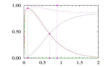
Figure 1: The energy densities $\Omega_{\hbox{\scriptsize x}}(\eta)$ are shown for the quintessence potential (57) for $w_{\phi}=-\frac{1}{3}$ using the parameters given in Sect. VI.

In the case $w_{\phi}<-\frac{1}{3}$, the universe becomes asymptotically flat, whereas for $w_{\phi}=-\frac{1}{3}$ it stays forever hyperbolic with $\Omega_{\hbox{\scriptsize tot}}(\infty)<1$, see Eq. (47). Radiation-quintessence equality occurs at $z=z_{{\hbox{\scriptsize r}}\phi}$ with

$$z_{{\hbox{\scriptsize r}}\phi}\;=\;\left(\frac{\Omega_{\phi}}{\Omega_{\hbox{\scriptsize r}}}\right)^{\frac{1}{1-3w_{\phi}}}\,-\,1\hskip 10.0pt.$$ (49)

The matter component takes its maximum value at a redshift value $z_{\hbox{\scriptsize m}}$, which can be obtained as a solution of the equation

$$\Omega_{\hbox{\scriptsize r}}(1+z_{\hbox{\scriptsize m}})^{1-3w_{\phi}}\,-\,\Omega_{\hbox{\scriptsize c}}(1+z_{\hbox{\scriptsize m}})^{-(1+3w_{\phi})}\;=\;-3\,w_{\phi}\,\Omega_{\phi}\hskip 10.0pt.$$ (50)

Matter-quintessence equality holds at $z=z_{\hbox{\scriptsize m}\phi}$ with

$$z_{\hbox{\scriptsize m}\phi}\;=\;\left(\frac{\Omega_{\phi}}{\Omega_{\hbox{\scriptsize m}}}\right)^{-1/(3w_{\phi})}\,-\,1\hskip 10.0pt.$$ (51)

Fig.1 shows the time-evolution of the energy densities $\Omega_{\hbox{\scriptsize x}}(\eta)$ for $w_{\phi}=-\frac{1}{3}$ using the parameters discussed in Sect. VI. During the epoch of quintessence dominance the growth of linear perturbations is suppressed. This suppression increases thus with increasing $w_{\phi}$ since then dark energy dominates earlier. In cases of too early dark energy dominance, one needs either a large bias parameter or models with a large CDM-contribution in order to obtain a power spectrum $P(k)$ of large scale structure that is consistent with the observations.

V Explicit Analytic Expressions for the Quintessence Potential

Formula (20) gives the quintessence potential $V(\phi)$ in terms of the scale factor $A(\phi)$, which in turn has to be obtained by “inversion” of the integral appearing in Eq. (22)

$$I_{w}(u) = I_{w}(u;\Omega_{\hbox{\scriptsize r}},\Omega_{\hbox{\scriptsize m}},\Omega_{\hbox{\scriptsize c}},\Omega_{\phi})$$

$$:= \int_{0}^{u}\frac{y^{-\frac{1}{2}-\frac{3}{2}w}}{\sqrt{\Omega_{\phi}y^{1-3w}+\Omega_{\hbox{\scriptsize c}}y^{2}+\Omega_{\hbox{\scriptsize m}}y+\Omega_{\hbox{\scriptsize r}}}}\;dy\hskip 10.0pt,$$

where in the following we assume $u\geq 0$, $w\in[-1,-\frac{1}{3}]$ and $\Omega_{\hbox{\scriptsize x}}>0$ for $\hbox{x}=\hbox{r},\hbox{m},\hbox{c},\phi$. The problem of integration posed by (V) is in general insoluble by means of elementary functions. For special values of $w$, however, it is possible to give explicit solutions to our problem.

V.1 The Potential for $w_{\phi}=-\frac{1}{3}$

In the case of a quintessence component belonging to a constant equation of state, $w_{\phi}=-\frac{1}{3}$, the integral (V) is particularly simple $(\tilde{\Omega}_{\phi}:=\Omega_{\phi}+\Omega_{\hbox{\scriptsize c}})$

$$I_{-\frac{1}{3}}\left(\frac{A(\phi)}{a_{0}}\right)\;=\;\frac{1}{\sqrt{\tilde{\Omega}_{\phi}}}\,\ln\left(\frac{X}{Y}\right)\hskip 10.0pt,$$ (53)

where we have introduced the abbreviations

$$X := 2\sqrt{Z}\,+\,2\tilde{\Omega}_{\phi}\,\left(\frac{A}{a_{0}}\right)\,+\,\Omega_{\hbox{\scriptsize m}}$$

$$Y := 2\sqrt{\tilde{\Omega}_{\phi}\Omega_{\hbox{\scriptsize r}}}\,+\,\Omega_{\hbox{\scriptsize m}}$$ (54)

$$Z := \tilde{\Omega}_{\phi}\left(\Omega_{\hbox{\scriptsize r}}\,+\,\Omega_{\hbox{\scriptsize m}}\,\left(\frac{A}{a_{0}}\right)\,+\,\tilde{\Omega}_{\phi}\,\left(\frac{A}{a_{0}}\right)^{2}\right)\hskip 10.0pt.$$

From Eqs. (53) and (22) one gets

$$X\;=\;Y\,e^{B\phi}\hskip 10.0pt,$$ (55)

where $B$ is given in Eq. (34) for $w_{\phi}=-\frac{1}{3}$. Furthermore, we obtain from (54) $(X-\Omega_{\hbox{\scriptsize m}})-2\tilde{\Omega}_{\phi}\,\left(\frac{A}{a_{0}}\right)=2\sqrt{Z}$, and squaring this equation yields

$$(X-\Omega_{\hbox{\scriptsize m}})^{2}\,-\,4\tilde{\Omega}_{\phi}\,(X-\Omega_{\hbox{\scriptsize m}})\,\left(\frac{A}{a_{0}}\right)\,+\,4\tilde{\Omega}_{\phi}^{2}\left(\frac{A}{a_{0}}\right)^{2} =$$

$$4\tilde{\Omega}_{\phi}\left(\Omega_{\hbox{\scriptsize r}}\,+\,\Omega_{\hbox{\scriptsize m}}\,\left(\frac{A}{a_{0}}\right)\,+\,\tilde{\Omega}_{\phi}\,\left(\frac{A}{a_{0}}\right)^{2}\right)\hskip 10.0pt,$$

which can easily be solved for $A/a_{0}$ giving

$$\frac{A(\phi)}{a_{0}}\;=\;\frac{1}{4\tilde{\Omega}_{\phi}}\left(X-2\Omega_{\hbox{\scriptsize m}}+(\Omega_{\hbox{\scriptsize m}}^{2}-4\tilde{\Omega}_{\phi}\Omega_{\hbox{\scriptsize r}})\,X^{-1}\right)\hskip 10.0pt.$$

Replacing then $X$ by the solution (55), leads to the following explicit expression for the scale factor $A(\phi)$ as a function of the quintessence field $\phi$

$$\frac{A(\phi)}{a_{0}}\;=\;\frac{\Omega_{\hbox{\scriptsize m}}}{2(\Omega_{\phi}+\Omega_{\hbox{\scriptsize c}})}\,\left(\tilde{\eta}\sinh(B\phi)+\cosh(B\phi)-1\right)$$ (56)

with $\tilde{\eta}:=\frac{2}{\Omega_{\hbox{\scriptsize m}}}\sqrt{\Omega_{\hbox{\scriptsize r}}(\Omega_{\phi}+\Omega_{\hbox{\scriptsize c}})}$. It remains to insert the result (56) into the general formula (20), to arrive at the exact quintessence potential for $w_{\phi}=-\frac{1}{3}$

$$V(\phi)\;=\;\frac{V_{0}}{\left[\tilde{\eta}\sinh(B\phi)+\cosh(B\phi)-1\right]^{2}}\hskip 10.0pt,$$ (57)

where we defined the potential strength $V_{0}=\frac{8}{3}\varepsilon_{\hbox{\scriptsize crit}}\Omega_{\phi}(\Omega_{\phi}+\Omega_{\hbox{\scriptsize c}})^{2}/\Omega_{\hbox{\scriptsize m}}^{2}$. Thus, in the case $w_{\phi}=-\frac{1}{3}$ the quintessence potential is completely known, not only in its functional form (57), but also with its parameters which are uniquely determined by $H_{0}$ and the present cosmological density parameters $\Omega_{\hbox{\scriptsize r}}$, $\Omega_{\hbox{\scriptsize m}}$, $\Omega_{\phi}$ and $\Omega_{\hbox{\scriptsize c}}=1-\Omega_{\hbox{\scriptsize r}}-\Omega_{\hbox{\scriptsize m}}-\Omega_{\phi}$. The potential (57) and therefore the cosmic evolution is governed by two very different energy scales: the small critical energy $\varepsilon_{\hbox{\scriptsize crit}}$ and the huge Planck mass $m_{P}$! Explicitly, one derives from (57)

$$V(\phi)\;=\;\left\{\begin{matrix}\frac{V_{0}}{(\tilde{\eta}B)^{2}}\,\frac{1}{\phi^{2}}\hbox{ for }\phi\to 0\\ \frac{4V_{0}}{(1+\tilde{\eta})^{2}}\,e^{-2B\phi}\hbox{ for }\phi\to\infty\end{matrix}\right.\hskip 10.0pt,$$ (58)

which is in accordance with the general behavior given by Eqs. (28) and (35), respectively.

It is interesting to consider the limit of the potential (57) for vanishing radiation. In this limit, we obtain the following exact quintessence potential for a two-component model consisting of matter and quintessence with $w_{\phi}=-\frac{1}{3}$

$$V(\phi)\;=\;\frac{V_{0}}{4}\,\frac{1}{\sinh^{4}\left(\frac{B\phi}{2}\right)}\hskip 10.0pt.$$ (59)

In Sect. V.2, we shall show that this potential leads to an almost constant equation of state $w_{\phi}(\eta)$ with $w_{\phi}(0)=-\frac{1}{9}$ and $w_{\phi}(\eta)\to-\frac{1}{3}$ for $\eta\to\infty$, if (59) is assumed to govern the time-evolution of a quintessence field, where a full three-component background model consisting of radiation, matter and quintessence is employed. (See Sect. V.2 for details.)

V.2 The Potential for $w_{\phi}=-\frac{2}{3}$ and $\Omega_{\hbox{\scriptsize r}}\equiv 0$

If the quintessence component possesses a constant equation of state, $w_{\phi}=-\frac{2}{3}$, the relevant integral (V) reads

$$I_{-\frac{2}{3}}(u)\;=\;\int_{0}^{u}\frac{\sqrt{y}}{\sqrt{\Omega_{\phi}y^{3}+\Omega_{\hbox{\scriptsize c}}y^{2}+\Omega_{\hbox{\scriptsize m}}y+\Omega_{\hbox{\scriptsize r}}}}\;dy\hskip 10.0pt.$$ (60)

The integral (60) can be transformed into an elliptic integral of the third kind which can be expressed in terms of the Weierstrass $\sigma$- and $\zeta$-function. There exists, however, no simple inversion formula leading to an explicit formula for $u$. Eq. (60) simplifies considerably, if we set $\Omega_{\hbox{\scriptsize r}}\equiv 0$, i. e. neglect radiation. We then have to solve the integral

$$\left.I_{-\frac{2}{3}}(u)\right|_{\Omega_{\hbox{\scriptsize r}}\equiv 0}\;=\;\int_{0}^{u}\frac{1}{\sqrt{\Omega_{\phi}y^{2}+\Omega_{\hbox{\scriptsize c}}y+\Omega_{\hbox{\scriptsize m}}}}\;dy\hskip 10.0pt,$$ (61)

which is identical to the integral $I_{-\frac{1}{3}}(u)$, if we make the replacements $\tilde{\Omega}_{\phi}=\Omega_{\phi}+\Omega_{\hbox{\scriptsize c}}\to\Omega_{\phi}$, $\Omega_{\hbox{\scriptsize m}}\to\Omega_{\hbox{\scriptsize c}}$ and $\Omega_{\hbox{\scriptsize r}}\to\Omega_{\hbox{\scriptsize m}}$. We can thus immediately obtain the corresponding scale factor by making the above replacements in formula (56) and then obtain

$$\frac{A(\phi)}{a_{0}}\;=\;\frac{1}{2}\,\frac{\Omega_{\hbox{\scriptsize c}}}{\Omega_{\phi}}\,\left(\check{\eta}\sinh(B\phi)+\cosh(B\phi)-1\right)$$ (62)

with $\check{\eta}:=2\frac{\sqrt{\Omega_{\phi}\Omega_{\hbox{\scriptsize m}}}}{\Omega_{\hbox{\scriptsize c}}}$ and $B=\frac{2\sqrt{2\pi}}{m_{P}}$. Inserting (62) into our general formula (20), gives then the exact quintessence potential for a two-component model consisting of matter and quintessence with $w_{\phi}=-\frac{2}{3}$

$$V(\phi)\;=\;\frac{\check{V}_{0}}{\check{\eta}\sinh(B\phi)+\cosh(B\phi)-1}$$ (63)

with $\check{V}_{0}:=\frac{5}{3}\frac{\Omega_{\phi}^{2}}{\Omega_{\hbox{\scriptsize c}}}\varepsilon_{\hbox{\scriptsize crit}}$. Explicitly, one obtains

$$V(\phi)\;=\;\left\{\begin{matrix}\frac{\check{V}_{0}}{\check{\eta}}\,\,\frac{1}{B\phi}\hbox{ for }\phi\to 0\\ \frac{2\check{V}_{0}}{1+\check{\eta}}\,e^{-B\phi}\hbox{ for }\phi\to\infty\end{matrix}\right.\hskip 10.0pt,$$ (64)

which is in accordance with the general behavior given by Eqs.(28), (35) and (36).

Since radiation has been neglected in the derivation of the potential (63), it appears at first sight that (63) can be applied only in the matter-dominated epoch and later, i. e. for $\eta>\eta_{\hbox{\scriptsize m}}$ respectively $z<z_{\hbox{\scriptsize m}}$ (see Eq. (50)). We can consider, however, a model in which the potential (63) is assumed to govern the time-evolution of the quintessence field for all times, irrespective of its derivation, and solve Eqs. (3)$-$(6) in a full three-component background model consisting of radiation, matter and quintessence. Radiation is then included correctly by means of the scale factor $a(\eta)$, and thus the new model is consistent for all times. It is clear, however, that the equation of state $w_{\phi}(\eta)$ can no more be constant for all $\eta\geq 0$. Nevertheless, it is obvious that for the potential (63) asymptotically holds

$$w_{\phi}(\eta)\;\to\;-\frac{2}{3}\hskip 10.0pt\hbox{ for }\hskip 10.0pt\eta\;\to\;\eta_{\infty}\hskip 10.0pt,$$ (65)

where we expect $w_{\phi}(\eta)$ to be almost constant, $w_{\phi}(\eta)\simeq-\frac{2}{3}$, already for $\eta\gtrsim\eta_{\hbox{\scriptsize m}}$. But in the radiation-dominated epoch $0\leq\eta\leq\eta_{\hbox{\scriptsize m}}$, the equation of state will deviate from its asymptotic value $-\frac{2}{3}$. It is then interesting to study the behavior of $w_{\phi}(\eta)$ in the limit $\eta\to 0$.

For this purpose, let us consider the more general situation of a quintessence potential $V(\phi)$ for a two-component model consisting of matter and quintessence with a constant equation of state $w_{\infty}$, $-1<w_{\infty}\leq-\frac{1}{3}$. It follows from Eqs. (26) and (28) that $V(\phi)$ diverges in the radiation-dominated epoch like

$$V(\phi)\;=\;\frac{\overline{V}_{0}}{\phi^{\overline{\gamma}}}\,+\,\dots\hskip 10.0pt,\hskip 10.0pt\overline{\gamma}\;=\;-\,\frac{2}{w_{\infty}}(1+w_{\infty})\hskip 10.0pt.$$ (66)

We then assume, as in the discussion above, that this potential is taken as a model for quintessence using, however, in Eqs. (3)$-$(6) the scale factor $a(\eta)$ for a three-component model which takes also radiation into account. One then obtains a time dependent equation of state, $w_{\phi}(\eta)$, which asymptotically obeys

$$w_{\phi}(\eta)\;\to\;w_{\infty}\hskip 10.0pt,\hskip 10.0pt\eta\;\to\;\eta_{\infty}\hskip 10.0pt.$$ (67)

(We expect $w_{\phi}(\eta)\simeq w_{\infty}$ to hold for $\eta\gtrsim\eta_{\hbox{\scriptsize m}}$.) To derive the behavior of $w_{\phi}(\eta)$ in the opposite limit, $\eta\to 0$, we make the ansatz $\phi(\eta)=b\eta^{\sigma}+\dots$ for $\eta\to 0$ with $b>0$, $\sigma>0$. Since the background model includes radiation, we have $a(\eta)=a^{\prime}(0)\eta+\dots$ in this limit. With (66), it is not difficult to see that the equation of motion (5) is satisfied iff $\sigma=4/(\overline{\gamma}+2)$ and $b^{\overline{\gamma}+2}=\overline{\gamma}{a^{\prime}}^{2}(0)\overline{V}_{0}/(\sigma(\sigma+1))$. It then follows for the ratio of the kinetic to the potential energy (see Eq.(39)) $r_{\phi}(\eta)\to r_{\phi}(0)$, $\eta\to 0$, with

$$r_{\phi}(0)\;=\;\frac{b^{\overline{\gamma}+2}\sigma^{2}}{2{a^{\prime}}^{2}(0)\overline{V}_{0}}\;=\;\frac{2\overline{\gamma}}{\overline{\gamma}+6}$$

which yields

$$w_{\phi}(\eta)\;\to\;w_{\phi}(0)\,=\,\frac{1}{3}(1+4w_{\infty})\hskip 10.0pt,\hskip 10.0pt\eta\to 0\hskip 10.0pt.$$ (68)

(Notice that $-1<w_{\phi}(0)\leq-\frac{1}{9}$ and $w_{\phi}(0)>w_{\infty}$ for $-1<w_{\infty}\leq-\frac{1}{3}$.) We thus conclude that the equation of state for the above models starts with the initial value (68) at $\eta=0$ and then decreases to its asymptotic value $w_{\infty}$. In the special case $w_{\infty}=-\frac{2}{3}$, discussed at the beginning of this Section, we have $w_{\phi}(0)=-\frac{5}{9}$, and for the potential (59) with $w_{\infty}=-\frac{1}{3}$ one gets $w_{\phi}(0)=-\frac{1}{9}$.

V.3 Potentials with a Positive Cosmological Constant

V.3.1 General Properties

In the foregoing discussion, we have considered a three-component model consisting of radiation, matter and quintessence. We will now study a four-component model, which takes into account also a non-vanishing (positive) cosmological constant $\Lambda$ corresponding to an energy density (vacuum energy density)

$$\varepsilon_{\Lambda}\;:=\;\frac{\Lambda}{8\pi G}\;=\;\hbox{const.}$$ (69)

with density parameter $\Omega_{\Lambda}=\frac{\Lambda}{3H_{0}^{2}}>0$. Assuming $-1<w_{\phi}\leq-\frac{1}{3}$, we have now to compute instead of (V) the more general integral

$$\tilde{I}_{w}(u)\>:=\>\int_{0}^{u}\frac{y^{-\frac{1}{2}-\frac{3}{2}w}\;dy}{\sqrt{\Omega_{\Lambda}y^{4}+\Omega_{\phi}y^{1-3w}+\Omega_{\hbox{\scriptsize c}}y^{2}+\Omega_{\hbox{\scriptsize m}}y+\Omega_{\hbox{\scriptsize r}}}}\hskip 5.0pt.$$ (70)

Let us begin with some general remarks. Obviously, the leading asymptotic behavior of $\tilde{I}_{w}(u)$ in the limit $u\to 0$ is the same as for $I_{w}(u)$, Eq. (V) (see also (26)), and thus we obtain in the radiation-dominated epoch again the power-law divergence (28) with the same power $\gamma$ as in the case of the three-component models. In the limit $u\to\infty$, however, we get a completely different behavior, which follows from the fact that $\tilde{I}_{w}(u)$, Eq. (70), stays finite in this limit. (Indeed, the integrand of $\tilde{I}_{w}(u)$ behaves for $y\to\infty$ like $y^{-\frac{5}{2}-\frac{3}{2}w}$, and thus the integral (70) converges at the upper limit since $\frac{5}{2}+\frac{3}{2}w>1$ for $w>-1$.) Similarly, it follows that the corresponding generalization of the integral (29) stays finite in the limit $a(\eta)\to\infty$, which implies that the conformal time $\eta$ approaches at late times the finite value $\eta_{\infty}$ given by

$$\eta_{\infty}=\sqrt{\Omega_{\hbox{\scriptsize c}}}\int_{0}^{\infty}\frac{dy}{\sqrt{\Omega_{\Lambda}y^{4}+\Omega_{\phi}y^{1-3w_{\phi}}+\Omega_{\hbox{\scriptsize c}}y^{2}+\Omega_{\hbox{\scriptsize m}}y+\Omega_{\hbox{\scriptsize r}}}}\hskip 2.0pt.$$ (71)

We thus conclude that the quintessence field $\phi(\eta)$ approaches in the limit $\eta\to\eta_{\infty}$ the finite value $\phi_{\infty}:=\phi(\eta_{\infty})$ given by (see Eqs. (22) and (23))

$$\phi_{\infty}=\frac{1}{B_{0}}\int_{0}^{\infty}\frac{y^{-\frac{1}{2}-\frac{3}{2}w_{\phi}}\;dy}{\sqrt{\Omega_{\Lambda}y^{4}+\Omega_{\phi}y^{1-3w_{\phi}}+\Omega_{\hbox{\scriptsize c}}y^{2}+\Omega_{\hbox{\scriptsize m}}y+\Omega_{\hbox{\scriptsize r}}}}\hskip 2.0pt.$$ (72)

With (72), the generalization of Eq. (22) can be rewritten

$$B_{0}\,\phi\;=\;B_{0}\,\phi_{\infty}-\hat{I}_{w_{\phi}}\left(\frac{A(\phi)}{a_{0}}\right)\hskip 10.0pt,$$ (73)

where we have defined the function

$$\hat{I}_{w}(u):=\int_{u}^{\infty}\frac{y^{-\frac{1}{2}-\frac{3}{2}w}\;dy}{\sqrt{\Omega_{\Lambda}y^{4}+\Omega_{\phi}y^{1-3w}+\Omega_{\hbox{\scriptsize c}}y^{2}+\Omega_{\hbox{\scriptsize m}}y+\Omega_{\hbox{\scriptsize r}}}}\hskip 5.0pt.$$ (74)

In the limit $u\to\infty$, one obtains for $w>-1$

$$\hat{I}_{w}(u)=\frac{2}{3}\,\frac{1}{(1+w)\sqrt{\Omega_{\Lambda}}}\,u^{-\frac{3}{2}(1+w)}\,+\,\dots\hskip 10.0pt,$$ (75)

which yields together with (73) the following asymptotic behavior of the scale factor $A(\phi)$

$$\frac{A(\phi)}{a_{0}}\;=\;O\left((\phi_{\infty}-\phi)^{-\frac{2}{3(1+w_{\phi})}}\right)\hskip 10.0pt,\hskip 10.0pt\phi\to\phi_{\infty}\hskip 10.0pt.$$ (76)

Inserting the last result in our general formula (20), gives for $\Lambda>0$, $w_{\phi}>-1$

$$V(\phi)\;=\;3\pi(1-w_{\phi}^{2})\Omega_{\Lambda}\varepsilon_{\hbox{\scriptsize crit}}\left(\frac{\phi_{\infty}-\phi}{m_{P}}\right)^{2}\,+\,\dots\hskip 2.0pt,\hskip 2.0pt\phi\to\phi_{\infty}\hskip 1.0pt.$$ (77)

Thus, the quintessence potential shows at late times $(\eta\to\eta_{\infty})$ in a universe with a positive cosmological constant a completely different behavior from that exhibited by Eq. (35). While $V(\phi)$ vanishes in the case $\Lambda\equiv 0$ exponentially for $\phi\to\infty$, it vanishes for $\Lambda>0$ only like a power, Eq. (77), at a finite value $\phi_{\infty}$ for $\phi\to\phi_{\infty}$.

In the case $\Lambda>0$, we have to replace Eq. (43) for the time-evolution of the density parameters by

$$\Omega_{\hbox{\scriptsize x}}(\eta)\;=\;\frac{y^{1-3w_{\hbox{\scriptsize x}}}}{g_{\Lambda}(y)}\,\Omega_{\hbox{\scriptsize x}}\hskip 10.0pt,\hskip 10.0pt\hbox{x}=\{\hbox{r},\hbox{m},\phi,\Lambda\}$$ (78)

and Eq. (44) for $\Omega_{\hbox{\scriptsize tot}}(\eta)$ by

$$\Omega_{\hbox{\scriptsize tot}}(\eta)\;=\;1\,-\,\frac{y^{2}}{g_{\Lambda}(y)}\,(1-\Omega_{\hbox{\scriptsize tot}})$$ (79)

with (see Eq.(21))

$$g_{\Lambda}(y)\;:=\;\Omega_{\Lambda}y^{4}\,+\,g(y)\;=\;\sum_{\hbox{\scriptsize x}=\hbox{\scriptsize r},\hbox{\scriptsize m},\phi,\Lambda,\hbox{\scriptsize c}}\Omega_{\hbox{\scriptsize x}}\,y^{1-3w_{\hbox{\scriptsize x}}}\hskip 10.0pt.$$ (80)

Obviously, the behavior (46) of the density parameters in the limit $\eta\to 0$ is not changed, and we only have to add $\Omega_{\Lambda}(\eta)=O(\eta^{4})$ for $\eta\to 0$. At late times, $z\to-1$, however, Eqs. (47) and (48) have to be replaced by $(w_{\phi}>-1)$

$$\begin{matrix}\Omega_{\hbox{\scriptsize r}}(\eta)&=&\frac{\Omega_{\hbox{\scriptsize r}}}{\Omega_{\Lambda}}\,(1+z)^{4}\,+\,\dots\;\to\;0\\ \Omega_{\hbox{\scriptsize m}}(\eta)&=&\frac{\Omega_{\hbox{\scriptsize m}}}{\Omega_{\Lambda}}\,(1+z)^{3}\,+\,\dots\;\to\;0\\ \Omega_{\phi}(\eta)&=&\frac{\Omega_{\phi}}{\Omega_{\Lambda}}\,(1+z)^{3+3w_{\phi}}\,+\,\dots\;\to\;0\\ \Omega_{\Lambda}(\eta)&=&1-\frac{\Omega_{\phi}}{\Omega_{\Lambda}}\,(1+z)^{3+3w_{\phi}}+\dots\to 1\\ \Omega_{\hbox{\scriptsize tot}}(\eta)&=&1-\frac{\Omega_{\hbox{\scriptsize c}}}{\Omega_{\Lambda}}\,(1+z)^{2}+\dots\to 1\end{matrix}\hskip 10.0pt.$$ (81)

We see that in the case $\Lambda>0$ also the quintessence component vanishes asymptotically at late times, in contrast to the earlier behavior (48), since now the vacuum contribution $\Omega_{\Lambda}(\eta)$ dominates and approaches one in this limit. Furthermore, we observe that for $\Lambda>0$ the universe becomes asymptotically flat. Quintessence-vacuum energy equality holds at $z=z_{\phi\Lambda}$ with

$$z_{\phi\Lambda}\;=\;\left(\frac{\Omega_{\Lambda}}{\Omega_{\phi}}\right)^{\frac{1}{3+3w_{\phi}}}\,-\,1\hskip 10.0pt.$$ (82)

V.3.2 The Potential for $w_{\phi}=-\frac{1}{3}$ and $\Lambda>0$

For $w_{\phi}=-\frac{1}{3}$ and $\Lambda>0$, we have (see Eqs. (22) and (70))

$$B_{0}\,\phi\;=\;\tilde{I}_{-\frac{1}{3}}\left(\frac{A(\phi)}{a_{0}}\right)\hskip 10.0pt,$$ (83)

and thus we have to “invert” the integral

$$\zeta\;:=\;\tilde{I}_{-\frac{1}{3}}(u)\;=\;\int_{0}^{u}\frac{dy}{\sqrt{\Omega_{\Lambda}y^{4}+\tilde{\Omega}_{\phi}y^{2}+\Omega_{\hbox{\scriptsize m}}y+\Omega_{\hbox{\scriptsize r}}}}\hskip 10.0pt.$$ (84)

The integral (84) is an elliptic integral of the first kind, which is insoluble by means of elementary functions. However, it is possible to invert it and to express $u$ as a rational function of ${\cal P}(\zeta)$, where ${\cal P}(\zeta)$ is the Weierstrass ${\cal P}$-function. It then follows from (83) that $A(\phi)/a_{0}$ can be expressed as a rational function of ${\cal P}(B_{0}\phi)$. (This method has already been used in our earlier paper Aurich_Steiner_2000 to express $a(\eta)$ in terms of ${\cal P}(\eta)$).

Let $F(y):=a_{0}y^{4}+4a_{1}y^{3}+6a_{2}y^{2}+4a_{3}y+a_{4}$ be any quartic polynomial which has no repeated factors; and let its invariants be Whittaker_Watson_1973

$$g_{2} := a_{0}a_{4}-4a_{1}a_{3}+3a_{2}^{2}$$

$$g_{3} := a_{0}a_{2}a_{4}+2a_{1}a_{2}a_{3}-a_{2}^{3}-a_{0}a_{3}^{2}-a_{1}^{2}a_{4}\hskip 10.0pt.$$ (85)

Furthermore, let

$$\zeta\;=\;\int_{\alpha}^{u}\frac{dy}{\sqrt{F(y)}}\hskip 10.0pt,$$ (86)

where $\alpha$ is any constant. (In the applications, which we have in mind, $\alpha$ is real and non-negative and $F(y)>0$ for $y\geq\alpha$.) Then Whittaker_Watson_1973

$$u = u(\zeta)=\alpha+\frac{\frac{1}{2}F^{\prime}(\alpha)\left({\cal P}(\zeta)-\frac{1}{24}F^{\prime\prime}(\alpha)\right)}{2\left({\cal P}(\zeta)-\frac{1}{24}F^{\prime\prime}(\alpha)\right)^{2}-\frac{1}{48}F(\alpha)F^{(4)}(\alpha)}$$ (87)

$$\hskip 10.0pt+\;\frac{\frac{1}{24}F(\alpha)F^{\prime\prime\prime}(\alpha)-\sqrt{F(\alpha)}{\cal P}^{\prime}(\zeta)}{2\left({\cal P}(\zeta)-\frac{1}{24}F^{\prime\prime}(\alpha)\right)^{2}-\frac{1}{48}F(\alpha)F^{(4)}(\alpha)}\hskip 5.0pt,$$

the Weierstrass function ${\cal P}(\zeta)={\cal P}(\zeta;g_{2},g_{3})$ being formed with the invariants (85) of the quartic $F(y)$. (Notice that we have corrected a sign on p. 454 in Whittaker_Watson_1973 by writing $-\sqrt{F(\alpha)}{\cal P}^{\prime}(\zeta)$ in Eq. (87).) ${\cal P}(\zeta)$ can numerically be evaluated very efficiently by its Laurent expansion

$${\cal P}(\zeta)\;=\;\frac{1}{\zeta^{2}}\,+\,\sum_{k=2}^{\infty}c_{k}\zeta^{2k-2}$$ (88)

with

$$c_{2}:=\frac{g_{2}}{20}\hskip 10.0pt,\hskip 10.0ptc_{3}:=\frac{g_{3}}{28}$$

and the recursion relation Abramowitz_Stegun_1965

$$c_{k}=\frac{3}{(2k+1)(k-3)}\sum_{m=2}^{k-2}c_{m}c_{k-m}\;\hbox{ for }\;k\geq 4\hskip 10.0pt.$$

With $a_{0}=\Omega_{\Lambda}$, $a_{1}=0$, $a_{2}=(\Omega_{\phi}+\Omega_{\hbox{\scriptsize c}})/6$, $a_{3}=\Omega_{\hbox{\scriptsize m}}/4$, $a_{4}=\Omega_{\hbox{\scriptsize r}}$ and $\alpha=0$, we obtain from Eqs. (83), (84), (86) and (87)

$$\frac{A(\phi)}{a_{0}}\;=\;\frac{\Omega_{\hbox{\scriptsize m}}}{4}\frac{{\cal P}(B_{0}\phi)-\frac{\Omega_{\phi}+\Omega_{\hbox{\scriptsize c}}}{12}-2\frac{\sqrt{\Omega_{\hbox{\scriptsize r}}}}{\Omega_{\hbox{\scriptsize m}}}{\cal P}^{\prime}(B_{0}\phi)}{\left({\cal P}(B_{0}\phi)-\frac{\Omega_{\phi}+\Omega_{\hbox{\scriptsize c}}}{12}\right)^{2}-\frac{\Omega_{\hbox{\scriptsize r}}\Omega_{\Lambda}}{4}}$$ (89)

with $B_{0}=\frac{2\sqrt{\pi}}{m_{P}}\Omega_{\phi}^{-1/2}$, where ${\cal P}(B_{0}\phi;g_{2},g_{3})$ has to be formed with the invariants

$$g_{2} := \frac{\left(\Omega_{\phi}+\Omega_{\hbox{\scriptsize c}}\right)^{2}}{12}+\Omega_{\hbox{\scriptsize r}}\Omega_{\Lambda}$$ (90)

$$g_{3} := -\frac{\left(\Omega_{\phi}+\Omega_{\hbox{\scriptsize c}}\right)^{3}}{216}+\left(\frac{\Omega_{\hbox{\scriptsize r}}\left(\Omega_{\phi}+\Omega_{\hbox{\scriptsize c}}\right)}{6}-\frac{\Omega_{\hbox{\scriptsize m}}^{2}}{16}\right)\Omega_{\Lambda}\hskip 10.0pt.$$

Inserting (89) into our general formula (20), yields the exact quintessence potential for a four-component model with $\Lambda>0$ and $w_{\phi}=-\frac{1}{3}$

$$V(\phi) = \frac{4V_{0}}{\left(\Omega_{\phi}+\Omega_{\hbox{\scriptsize c}}\right)^{2}}\,$$

$$\times\;\left[\frac{\left({\cal P}(B_{0}\phi)-\frac{\Omega_{\phi}+\Omega_{\hbox{\scriptsize c}}}{12}\right)^{2}-\frac{\Omega_{\hbox{\scriptsize r}}\Omega_{\Lambda}}{4}}{{\cal P}(B_{0}\phi)-\frac{\Omega_{\phi}+\Omega_{\hbox{\scriptsize c}}}{12}-2\frac{\sqrt{\Omega_{\hbox{\scriptsize r}}}}{\Omega_{\hbox{\scriptsize m}}}{\cal P}^{\prime}(B_{0}\phi)}\right]^{2}\hskip 10.0pt,$$

where the potential strength $V_{0}$ is found to be the same as in Eq.(57). Using the leading behavior ${\cal P}(B_{0}\phi)=(B_{0}\phi)^{-2}+\dots$ and ${\cal P}^{\prime}(B_{0}\phi)=-2(B_{0}\phi)^{-3}+\dots$ for $\phi\to 0$, it follows that (V.3.2) obeys the correct power-law behavior (28) (see also Eq. (58)) in the radiation-dominated epoch $\phi\to 0$. To derive the asymptotic behavior of $V(\phi)$ in the opposite limit at late times, $\eta\to\eta_{\infty}$ or $\phi\to\phi_{\infty}$, (see Eqs. (71) and (72)), we use Whittaker_Watson_1973

$${\cal P}(\zeta)\;=\;\frac{\sqrt{F(u)F(\alpha)}+F(\alpha)}{2(u-\alpha)^{2}}+\frac{F^{\prime}(\alpha)}{4(u-\alpha)}+\frac{F^{\prime\prime}(\alpha)}{24}$$

$${\cal P}^{\prime}(\zeta) = -\left[\frac{F(u)}{(u-\alpha)^{3}}-\frac{F^{\prime}(u)}{4(u-\alpha)^{2}}\right]\sqrt{F(\alpha)}$$

$$-\left[\frac{F(\alpha)}{(u-\alpha)^{3}}+\frac{F^{\prime}(\alpha)}{4(u-\alpha)^{2}}\right]\sqrt{F(u)}$$

with the same notation as in Eq. (86). From Eqs. (83) and (84) we infer that we have to choose $\alpha=0$ in Eq. (V.3.2) and then consider the limit $u=A(\phi)/a_{0}\to\infty$, which yields

$${\cal P}(B_{0}\phi_{\infty}) = \frac{\sqrt{F(0)}}{2}\,\lim_{u\to\infty}\,\frac{\sqrt{F(u)}}{u^{2}}+\frac{F^{\prime\prime}(0)}{24}$$ (93)

$$= \frac{\sqrt{\Omega_{\hbox{\scriptsize r}}\Omega_{\Lambda}}}{2}+\frac{\Omega_{\phi}+\Omega_{\hbox{\scriptsize c}}}{12}$$

and

$${\cal P}^{\prime}(B_{0}\phi_{\infty}) = -\sqrt{F(0)}\,\lim_{u\to\infty}\,\left[\frac{F(u)}{u^{3}}-\frac{F^{\prime}(u)}{4u^{2}}\right]$$ (94)

$$-\frac{F^{\prime}(0)}{4}\,\lim_{u\to\infty}\,\frac{\sqrt{F(u)}}{u^{2}}$$

$$= -\,\frac{\Omega_{\hbox{\scriptsize m}}}{4}\sqrt{\Omega_{\Lambda}}\hskip 10.0pt.$$

The implicit relation (93) turns out to be very convenient to calculate $\phi_{\infty}$ numerically (instead of computing the integral (72)). A Taylor expansion of ${\cal P}(B_{0}\phi)$ and ${\cal P}^{\prime}(B_{0}\phi)$ at $\phi=\phi_{\infty}$ gives then for the potential (V.3.2) the desired result in the limit $\phi\to\phi_{\infty}$. Explicitly, one derives

$$V(\phi)\;=\;\left\{\begin{matrix}\frac{V_{0}\Omega_{\hbox{\scriptsize m}}^{2}}{16\Omega_{\hbox{\scriptsize r}}}\,\frac{1}{(B_{0}\phi)^{2}}\hbox{ for }\phi\to 0\\ \frac{2}{3}\varepsilon_{\hbox{\scriptsize crit}}\Omega_{\phi}\Omega_{\Lambda}\left(B_{0}(\phi_{\infty}-\phi)\right)^{2}\hbox{ for }\phi\to\phi_{\infty}\end{matrix}\right.$$ (95)

in full agreement with the general behavior (28) and (77).

It is worthwhile to check whether the potential (V.3.2) goes in the limit of a vanishing cosmological constant, $\Omega_{\Lambda}\to 0$, over to our previous result (57). From (90), we obtain for the invariants in this limit $g_{2}\to(\Omega_{\phi}+\Omega_{\hbox{\scriptsize c}})^{2}/12$ and $g_{3}\to-(\Omega_{\phi}+\Omega_{\hbox{\scriptsize c}})^{3}/216$. Using the homogeneity property of the function ${\cal P}(\zeta)$ Whittaker_Watson_1973 , ${\cal P}(\zeta;g_{2},g_{3})=\lambda^{2}{\cal P}(\lambda\zeta;\frac{g_{2}}{\lambda^{4}},\frac{g_{3}}{\lambda^{6}})$, we obtain with $\lambda=\sqrt{\Omega_{\phi}+\Omega_{\hbox{\scriptsize c}}}$

$${\cal P}(B_{0}\phi;g_{2},g_{3})\;\to_{(\Omega_{\Lambda}\to 0)}\;(\Omega_{\phi}+\Omega_{\hbox{\scriptsize c}})\,{\cal P}(B\phi;\frac{1}{12},-\frac{1}{216})\hskip 5.0pt,$$ (96)

where we have used the definition $B:=B_{0}\sqrt{\Omega_{\phi}+\Omega_{\hbox{\scriptsize c}}}$, see Eq. (34). Since the last ${\cal P}$-function can be expressed in terms of an elementary function Abramowitz_Stegun_1965 ,

$${\cal P}\left(\zeta;\frac{1}{12},-\frac{1}{216}\right)\;=\;\frac{1}{12}\,+\,\frac{1}{4\sinh^{2}\frac{\zeta}{2}}\hskip 10.0pt,$$ (97)

one obtains, indeed, that the potential (V.3.2) goes over to the potential (57) if the cosmological constant approaches zero.

V.3.3 The Potential for $w_{\phi}=-\frac{2}{3}$, $\Lambda>0$ and $\Omega_{\hbox{\scriptsize r}}\equiv 0$

For $w_{\phi}=-\frac{2}{3}$, we have to solve (see Eqs. (73) and (74))

$$B_{0}(\phi_{\infty}-\phi)\;=\;\hat{I}_{-\frac{2}{3}}\left(\frac{A(\phi)}{a_{0}}\right)$$ (98)

with

$$\hat{I}_{-\frac{2}{3}}(u)=\int_{u}^{\infty}\frac{\sqrt{y}\;dy}{\sqrt{\Omega_{\Lambda}y^{4}+\Omega_{\phi}y^{3}+\Omega_{\hbox{\scriptsize c}}y^{2}+\Omega_{\hbox{\scriptsize m}}y+\Omega_{\hbox{\scriptsize r}}}}\hskip 10.0pt.$$ (99)

The last integral simplifies considerably, if we set $\Omega_{r}\equiv 0$, i. e. neglect radiation. Introducing the new variable of integration $t$, $y:=\frac{4}{\Omega_{\Lambda}}\left(t-\frac{\Omega_{\phi}}{12}\right)$, the integrand is transformed into Weierstrass normal form

$$B_{0}(\phi_{\infty}-\phi)\;=\;\int_{T}^{\infty}\frac{dt}{\sqrt{4t^{3}-g_{2}t-g_{3}}}$$ (100)

with invariants

$$g_{2} := \frac{\Omega_{\phi}^{2}}{12}-\frac{\Omega_{\hbox{\scriptsize c}}\Omega_{\Lambda}}{4}$$ (101)

$$g_{3} := -\frac{\Omega_{\phi}^{3}}{216}+\frac{1}{48}\left(\Omega_{\hbox{\scriptsize c}}\Omega_{\phi}-3\Omega_{\hbox{\scriptsize m}}\Omega_{\Lambda}\right)\Omega_{\Lambda}$$

and $T:=\frac{\Omega_{\Lambda}}{4}\left(\frac{A(\phi)}{a_{0}}\right)+\frac{\Omega_{\phi}}{12}$. In the form (100), the integral can be solved Whittaker_Watson_1973 in terms of the Weierstrass ${\cal P}$-function, $T={\cal P}(B_{0}(\phi_{\infty}-\phi))$, and one immediately obtains for the scale factor

$$\frac{A(\phi)}{a_{0}}\;=\;\frac{4}{\Omega_{\Lambda}}\,{\cal P}(B_{0}(\phi_{\infty}-\phi))\,-\,\frac{1}{3}\,\frac{\Omega_{\phi}}{\Omega_{\Lambda}}\hskip 10.0pt,$$ (102)

where the function ${\cal P}$ has to be formed with the invariants (101). Inserting (102) into our general formula (20), yields the exact quintessence potential for a three-component model consisting of matter, quintessence and a cosmological constant with $w_{\phi}=-\frac{2}{3}$, $\Omega_{\Lambda}>0$ and $\Omega_{\hbox{\scriptsize r}}\equiv 0$

$$V(\phi)\;=\;\frac{\hat{V}_{0}}{{\cal P}(B_{0}(\phi_{\infty}-\phi))-\frac{\Omega_{\phi}}{12}}$$ (103)

with $\hat{V}_{0}=\frac{5}{24}\varepsilon_{\hbox{\scriptsize crit}}\Omega_{\phi}\Omega_{\Lambda}$. The potential (103) depends on the field $\phi_{\infty}$, which is defined by

$$\phi_{\infty} = \frac{1}{B_{0}}\int_{0}^{\infty}\frac{dy}{\sqrt{\Omega_{\Lambda}y^{3}+\Omega_{\phi}y^{2}+\Omega_{\hbox{\scriptsize c}}y+\Omega_{\hbox{\scriptsize m}}}}$$ (104)

$$= \frac{1}{B_{0}}\int_{\Omega_{\phi}/12}^{\infty}\frac{dt}{\sqrt{4t^{3}-g_{2}t-g_{3}}}$$

and can be computed from

$${\cal P}(B_{0}\phi_{\infty})\;=\;\frac{\Omega_{\phi}}{12}\hskip 10.0pt.$$ (105)

Expanding ${\cal P}(B_{0}(\phi_{\infty}-\phi))$ into a Taylor series at $\phi=0$ and using (105) and

$${\cal P}^{\prime}(B_{0}\phi_{\infty})\;=\;-\,\frac{\sqrt{\Omega_{\hbox{\scriptsize m}}}}{4}\,\Omega_{\Lambda}\hskip 10.0pt,$$ (106)

one derives the asymptotic behavior of the potential (103) for $\phi\to 0$. The behavior of $V(\phi)$ in the limit $\phi\to\phi_{\infty}$ follows immediately form (88). Explicitly, one obtains

$$V(\phi)\;=\;\left\{\begin{matrix}\frac{4\hat{V}_{0}}{\sqrt{\Omega_{\hbox{\scriptsize m}}}\Omega_{\Lambda}}\,\frac{1}{B_{0}\phi}\hbox{ for }\phi\to 0\\ \hat{V}_{0}\,\left(B_{0}(\phi_{\infty}-\phi)\right)^{2}\hbox{ for }\phi\to\phi_{\infty}\end{matrix}\right.\hskip 10.0pt,$$ (107)

which is in accordance with the general behavior given by (28) and (77).

VI Comparison with cosmological observations

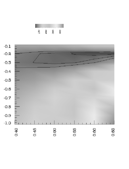
Figure 2: The $\chi^{2}$ values are shown in dependence on $w_{\phi}$ and $\Omega_{\phi}$ for $\Omega_{\hbox{\scriptsize tot}}=0.85$ using RadPack for 41 data points. The curves with $\chi^{2}=40$, 50 and 60 are indicated. The minimum $\chi^{2}_{\hbox{\scriptsize min}}=36$ occurs at $\Omega_{\phi}=0.6$ and $w_{\phi}=-0.2$.

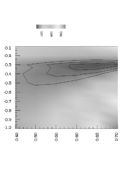
Figure 3: The $\chi^{2}$ values are shown in dependence on $w_{\phi}$ and $\Omega_{\phi}$ for $\Omega_{\hbox{\scriptsize tot}}=0.9$ using RadPack for 41 data points. The curves with $\chi^{2}=40$, 50 and 60 are indicated. The minimum $\chi^{2}_{\hbox{\scriptsize min}}=33$ occurs at $\Omega_{\phi}=0.65$ and $w_{\phi}=-0.3$.

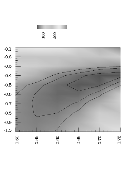
Figure 4: The $\chi^{2}$ values are shown in dependence on $w_{\phi}$ and $\Omega_{\phi}$ for $\Omega_{\hbox{\scriptsize tot}}=0.95$ using RadPack for 41 data points. The curves with $\chi^{2}=40$, 50 and 60 are indicated. The minimum $\chi^{2}_{\hbox{\scriptsize min}}=35$ occurs at $\Omega_{\phi}=0.7$ and $w_{\phi}=-0.4$.

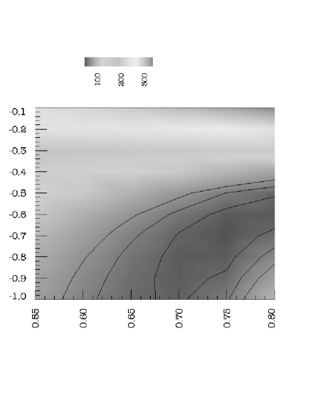
Figure 5: The $\chi^{2}$ values are shown in dependence on $w_{\phi}$ and $\Omega_{\phi}$ for $\Omega_{\hbox{\scriptsize tot}}=1.0$ using RadPack for 41 data points. The curves with $\chi^{2}=40$, 50 and 60 are indicated. The minimum $\chi^{2}_{\hbox{\scriptsize min}}=34$ occurs at $\Omega_{\phi}=0.75$ and $w_{\phi}=-0.7$.

After having discussed various aspects of quintessence models with a constant equation of state $w_{\phi}$, let us come to a detailed comparison with the CMB observations. (A preliminary announcement of our results can be found in Steiner_Aurich_2002 .) We use in our comparison the following priors. The Hubble constant $H_{0}=h\times 100\hbox{ km s}^{-1}\hbox{Mpc}^{-1}$ is set to $h=0.65$, and $\Omega_{\hbox{\scriptsize b}}=0.05$ (i. e. $\Omega_{\hbox{\scriptsize b}}h^{2}=0.021$) is chosen in agreement with the current Big-Bang nucleosynthesis constraints.

The CMB anisotropy is computed according to Ma_Bertschinger_1995 ; Hu_1998 using the conformal Newtonian gauge. The relativistic components are photons and three massless neutrino families with standard thermal history. For the photons, the polarization dependence on the Thomson cross section is taken into account. The recombination history of the universe is computed using RECFAST Seager_Sasselov_Scott_1999 . The non-relativistic components are baryonic and cold dark matter. The initial conditions are given by an initial curvature perturbation with no initial entropy perturbations in relativistic and non-relativistic components. Furthermore, we assume that there are no tensor mode contributions. The initial curvature perturbation is assumed to be scale-invariant which is “naturally” suggested by inflationary models. The quintessence fluctuations are initially set to zero. Other choices for the quintessence inhomogeneity would yield practically the same results because these models are insensitive to the initial conditions on the quintessence fluctuations Dave_Caldwell_Steinhardt_2002 .

The CMB anisotropy of these quintessence models is compared with the angular power spectrum $\delta T_{l}=\sqrt{l(l+1)C_{l}/2\pi}$ obtained by the experiments BOOMERanG Netterfield_et_al_2001 , MAXIMA-1 Lee_et_al_2001 , and DASI Halverson_et_al_2001 . This corresponds to 41 data points. The amplitude of the initial curvature perturbation is fitted such that the value of $\chi^{2}$ is minimized with respect to these three experiments, where $\chi^{2}$ is computed using RADPACK.

Figure 6: The angular power spectrum $\delta T_{l}/T$ is presented for the four best models for the cases $\Omega_{\hbox{\scriptsize tot}}=0.85$, $\Omega_{\hbox{\scriptsize tot}}=0.9$, $\Omega_{\hbox{\scriptsize tot}}=0.95$, and $\Omega_{\hbox{\scriptsize tot}}=1.0$. These are determined by the minimum of $\chi^{2}$ shown in figures 2 to 5. The data are taken from Netterfield_et_al_2001 ; Lee_et_al_2001 ; Halverson_et_al_2001 .

The figures 2 to 5 present the values of $\chi^{2}$ for the four cases $\Omega_{\hbox{\scriptsize tot}}=0.85$, $\Omega_{\hbox{\scriptsize tot}}=0.9$, $\Omega_{\hbox{\scriptsize tot}}=0.95$, and $\Omega_{\hbox{\scriptsize tot}}=1.0$, respectively. The values of $\chi^{2}$ are shown in dependence on $w_{\phi}$ and $\Omega_{\phi}$. Since $\Omega_{\hbox{\scriptsize tot}}$ is held fixed, the matter density $\Omega_{\hbox{\scriptsize m}}$ is given by $\Omega_{\hbox{\scriptsize m}}=\Omega_{\hbox{\scriptsize tot}}-\Omega_{\phi}$ neglecting the small radiation contribution. One observes that a decreasing $\Omega_{\hbox{\scriptsize tot}}$ demands an increasing $w_{\phi}$, i. e. a less negative value; from $\Omega_{\hbox{\scriptsize tot}}=0.85$ to $\Omega_{\hbox{\scriptsize tot}}=1.0$ the equation of state shifts from $w_{\phi}=-0.2$ to $w_{\phi}=-0.7$. Furthermore, all acceptable models require a dominant dark energy component $\Omega_{\phi}\gtrsim 0.6$ and possess $\Omega_{\hbox{\scriptsize m}}=0.25$. Since the minimum of $\chi^{2}$ is for all four cases of the same order, $\chi^{2}_{\hbox{\scriptsize min}}=33\dots 36$, no definite value for the curvature is singled out. Thus we do not find convincing hints pointing towards vanishing curvature, i. e. a flat universe. The four best models corresponding to the cases $\Omega_{\hbox{\scriptsize tot}}=0.85$, $\Omega_{\hbox{\scriptsize tot}}=0.9$, $\Omega_{\hbox{\scriptsize tot}}=0.95$, and $\Omega_{\hbox{\scriptsize tot}}=1.0$, respectively, are nearly degenerated with respect to their angular power spectrum $\delta T_{l}/T$ as can be seen in figure 6. With the current observational accuracy, one cannot discriminate between these models. A degeneracy between $\Omega_{\phi}$ and $w_{\phi}$ exists already in the flat case, see e. g. Hu_Eisenstein_Tegmark_White_1999 ; Bean_Melchiorri_2002 ; Melchiorri_Mersini_Odman_Trodden_2002 . If the assumption of flatness is dropped, a degeneracy with respect to $\Omega_{\hbox{\scriptsize c}}$, $\Omega_{\phi}$ and $w_{\phi}$ arises. A special case, the degeneracy with respect to $\Omega_{\Lambda}$ and the curvature $\Omega_{\hbox{\scriptsize c}}$ is discussed in Efstathiou_Bond_1999 . The full $(\Omega_{\hbox{\scriptsize c}},\Omega_{\phi},w_{\phi})$-degeneracy can be inferred from Huterer_Turner_2001 in the neighborhood of a special flat model, where the shift $\Delta l_{1}$ of the first peak (see their Eq. (18)) from a flat $\Lambda$CDM model with $\Omega_{\hbox{\scriptsize m}}=0.3$ is analyzed. This geometrical degeneracy arises through the angular-diameter distance to the surface of last scattering having redshift $z_{\hbox{\scriptsize sls}}$,

$$d_{A}\,=\,\frac{1}{H_{0}\sqrt{|\Omega_{\hbox{\scriptsize c}}|}(z_{\hbox{\scriptsize sls}}+1)}S_{k}\left(\sqrt{|\Omega_{\hbox{\scriptsize c}}|}\int_{\frac{1}{1+z_{\hbox{\tiny sls}}}}^{1}\frac{dy}{\sqrt{g(y)}}\right)\hskip 3.0pt,$$ (108)

where $S_{k}(x)$ is $\sinh(x)$, $x$, $\sin(x)$ for $k=-1,0,+1$, respectively, if we include also the flat and the positive curvature case. The models with the lowest values of $\chi^{2}$ possess nearly the same angular-diameter distance $d_{A}$ to the surface of last scattering. Furthermore, the models which for fixed $\Omega_{\hbox{\scriptsize c}}$ match the anisotropy, have all the same $\Omega_{\hbox{\scriptsize m}}=0.25$. In figure 7 we show the angular-diameter distance $d_{A}$ to the surface of last scattering for this value of $\Omega_{\hbox{\scriptsize m}}$. Our models with the smallest $\chi^{2}$ lie close to the black marked contour of constant $d_{A}$. One infers from figure 7 that to the model with $\Omega_{\hbox{\scriptsize c}}=0$ and $w_{\phi}=-0.7$ correspond models with the same $d_{A}$ having $\Omega_{\hbox{\scriptsize c}}=0.05,0.1,0.15$ and $w_{\phi}\simeq-0.43,-0.3,-0.22$, respectively. Thus, this geometrical degeneracy allows also universes of negative curvature.

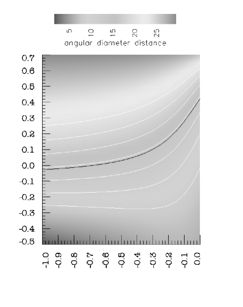
Figure 7: The angular-diameter distance $d_{A}$ is shown for models with $\Omega_{\hbox{\scriptsize m}}=0.25$ in dependence on $w_{\phi}$ and $\Omega_{\hbox{\scriptsize c}}$. The curves show the contours of constant $d_{A}$. Our models with the smallest $\chi^{2}$ value lie close to the black curve. ($z_{\hbox{\scriptsize sls}}=1100$ is assumed.)

One observes in figure 7 that the contours of constant $d_{A}$ have a larger slope for larger $w_{\phi}$, i. e. for the models with more negative curvature. This leads to more sharply confined regions of small values of $\chi^{2}$ in the parameter space with increasing $\Omega_{\hbox{\scriptsize c}}$, i. e. decreasing $\Omega_{\hbox{\scriptsize tot}}$. This trend is clearly visible in figures 2 to 5.

In figure 8 the magnitude-redshift relation $m_{\hbox{\scriptsize B}}(z)$ is shown for the four best models. One observes a very similar behavior in the three cases with negative curvature consistent with the supernovae Ia observations Hamuy_et_al_1996 ; Riess_et_al_1998 ; Perlmutter_et_al_1999 . The upper dotted curve belonging to the flat case gives a slightly better fit than the curves belonging to the cases with negative curvature but the latter are nevertheless consistent with these observations. At this point, it is important to be aware of the ongoing discussions whether the extinction in the host galaxies is indeed negligible for high $z$ supernovae Sullivan_et_al_2002 or whether this indicates an inconsistent treatment of host galaxy extinction when the extinction is only taken into account for low $z$ supernovae Rowan-Robinson_2002 ; Farrah_Meikle_Clements_Rowan-Robinson_Mattila_2002 . Furthermore, the hints for an accelerated expansion are also weakened if supernovae not observed before maximum light are excluded from the analysis Rowan-Robinson_2002 . Thus, it is probably save not to reject universes with negative curvature which need only a $0.1-0.2$ mag shift in order to be in perfect agreement with the observations. At this point it should be noted, as e. g. emphasized recently in Ellis_Stoeger_McEwan_Dunsby_2002 that while inflation is taken to predict that the universe is very close to flat, it does not imply that the spatial sections are exactly flat.

Figure 8: The magnitude-redshift relation $m_{\hbox{\scriptsize B}}(z)$ is shown for the four best models possessing $\Omega_{\hbox{\scriptsize tot}}=0.85$, $\Omega_{\hbox{\scriptsize tot}}=0.9$, $\Omega_{\hbox{\scriptsize tot}}=0.95$, and $\Omega_{\hbox{\scriptsize tot}}=1.0$ in comparison with the supernovae Ia data Hamuy_et_al_1996 ; Riess_et_al_1998 ; Perlmutter_et_al_1999 .

Let us now turn to the special case $w_{\phi}=-\frac{1}{3}$, i. e. to the potential (57) derived in Sect. V.1. Here we choose the following values for the cosmological parameters: $\Omega_{\hbox{\scriptsize cdm}}=0.25$, i. e. $\Omega_{\hbox{\scriptsize m}}=0.30$; $\Omega_{\phi}=0.60$, i. e. $\Omega_{\hbox{\scriptsize tot}}=0.90$ or $\Omega_{\hbox{\scriptsize c}}=0.10$, which gives $\Omega_{\hbox{\scriptsize tot}}(\infty)=\frac{6}{7}\simeq 0.86$. We then obtain $\eta_{\hbox{\scriptsize eq}}=0.0087$; $z_{\hbox{\scriptsize rec}}=1089$, i. e. $\eta_{\hbox{\scriptsize rec}}=0.0198$; $z_{\hbox{\scriptsize m}}=\sqrt{(\Omega_{\phi}+\Omega_{\hbox{\scriptsize c}})/\Omega_{\hbox{\scriptsize r}}}-1\simeq 83$, i. e. $\eta_{\hbox{\scriptsize m}}=0.106$; $z_{\hbox{\scriptsize m}\phi}=1$, i. e. $\eta_{\hbox{\scriptsize m}\phi}=0.687$; $\eta_{0}=0.8938$ corresponding to an age of the universe of $t_{0}=12.16\hbox{ Gyr}$. In Fig. 1 we show the density parameters $\Omega_{\hbox{\scriptsize x}}(\eta)$ as a function of conformal time $\eta$. Fig. 9 shows the prediction of the model for the angular power spectrum $\delta T_{l}=\sqrt{l(l+1)C_{l}/2\pi}$ of the CMB anisotropy in comparison with the BOOMERanG Netterfield_et_al_2001 , MAXIMA-1 Lee_et_al_2001 , and DASI Halverson_et_al_2001 experiments. One observes that the model describes the data very well ($\chi^{2}=35$ for $N_{\hbox{\scriptsize data}}=41$). The first three acoustic peaks occur at $l_{1}=222$, $l_{2}=538$ and $l_{3}=820$, in excellent agreement with the observations. In Fig. 10 we show the magnitude-redshift relation $m_{\hbox{\scriptsize B}}(z)$ in comparison with the supernovae Ia data Hamuy_et_al_1996 ; Riess_et_al_1998 ; Perlmutter_et_al_1999 . Again we observe good agreement with the data.

Figure 9: The angular power spectrum $\delta T_{l}/T$ for the quintessence potential (57) for $w_{\phi}=-\frac{1}{3}$ in comparison with the experiments Netterfield_et_al_2001 ; Lee_et_al_2001 ; Halverson_et_al_2001 as discussed in the text.

Figure 10: The $m_{\hbox{\scriptsize B}}(z)$ relation in comparison with the supernovae Ia data Hamuy_et_al_1996 ; Riess_et_al_1998 ; Perlmutter_et_al_1999 for the quintessence potential (57) for $w_{\phi}=-\frac{1}{3}$.

To summarize, we conclude that the quintessence model with $w_{\phi}=-\frac{1}{3}$ and $\Omega_{\hbox{\scriptsize tot}}=0.90$ is in excellent agreement with present observations. We have thus demonstrated that it is too early to claim that present data have already established that the universe is flat. It remains to be seen whether future observations give additional support to the idea that our universe is close to flat, but not exactly flat, and that its spatial geometry is hyperbolic.

References

- (1) C. B. Netterfield, P. A. R. Ade, J. J. Bock, J. R. Bond, J. Borrill, A. Boscaleri, K. Coble, C. R. Contaldi, B. P. Crill, P. de Bernardis, P. Farese, K. Ganga, et al., Astrophys. J. 571, 604 (2002), eprint astro-ph/0104460.
- (2) A. T. Lee, P. Ade, A. Balbi, J. Bock, J. Borrill, A. Boscaleri, P. de Bernardis, P. G. Ferreira, S. Hanany, V. V. Hristov, A. H. Jaffe, P. D. Mauskopf, et al., Astrophys. J. Lett. 561, L1 (2001), eprint astro-ph/0104459.
- (3) N. W. Halverson, E. M. Leitch, C. Pryke, J. Kovac, J. E. Carlstrom, W. L. Holzapfel, M. Dragovan, J. K. Cartwright, B. S. Mason, S. Padin, T. J. Pearson, M. C. Shepherd, et al., Astrophys. J. 568, 38 (2002), eprint astro-ph/0104489.
- (4) J. A. Peacock and S. J. Dodds, Mon. Not. R. Astron. Soc. 267, 1020 (1994).
- (5) A. J. S. Hamilton, M. Tegmark, and N. Padmanabhan, Mon. Not. R. Astron. Soc. 317, L23 (2000).
- (6) W. J. Percival, C. M. Baugh, J. Bland-Hawthorn, T. Bridges, R. Cannon, S. Cole, M. Colless, C. Collins, W. Couch, G. Dalton, R. De Propris, S. P. Driver, et al., Mon. Not. R. Astron. Soc. 327, 1297 (2001), eprint astro-ph/0105252.
- (7) G. Efstathiou, S. Moody, J. A. Peacock, W. J. Percival, C. Baugh, J. Bland-Hawthorn, T. Bridges, R. Cannon, S. Cole, M. Colless, C. Collins, W. Couch, et al., Mon. Not. R. Astron. Soc. 330, L29 (2002).
- (8) M. Hamuy, M. M. Phillips, N. B. Suntzeff, R. A. Schommer, J. Maza, and R. Aviles, Astron. J. 112, 2391 (1996).
- (9) A. G. Riess, A. V. Filippenko, P. Challis, A. Clocchiatti, A. Diercks, P. M. Garnavich, R. L. Gilliland, C. J. Hogan, S. Jha, R. P. Kirshner, B. Leibundgut, M. M. Phillips, et al., Astron. J. 116, 1009 (1998).
- (10) S. Perlmutter, G. Aldering, G. Goldhaber, R. A. Knop, P. Nugent, P. G. Castro, S. Deustua, S. Fabbro, A. Goobar, D. E. Groom, I. M. Hook, A. G. Kim, et al., Astrophys. J. 517, 565 (1999).
- (11) P. J. E. Peebles and B. Ratra, astro-ph/0207347 (2002).
- (12) P. Brax, J. Martin, and A. Riazuelo, Phys. Rev. D 62, 103505 (2000).
- (13) B. Ratra and P. J. E. Peebles, Phys. Rev. D 37, 3406 (1988).
- (14) R. R. Caldwell, R. Dave, and P. J. Steinhardt, Phys. Rev. Lett. 80, 1582 (1998).
- (15) L. Wang and P. J. Steinhardt, Astrophys. J. 508, 483 (1998).
- (16) A. Vilenkin, Phys. Rev. Lett. 53, 1016 (1984).
- (17) D. Spergel and U. Pen, Astrophys. J. Lett. 491, L67 (1997).
- (18) R. Durrer, M. Kunz, and A. Melchiorri, Physics Report 364, 1 (2002).
- (19) A. Gangui, astro-ph/0110285 (2001).
- (20) M. Doran, M. Lilley, J. Schwindt, and C. Wetterich, Astrophys. J. 559, 501 (2001).
- (21) M. Doran and M. Lilley, Mon. Not. R. Astron. Soc. 330, 965 (2002).
- (22) N. J. Cornish, Phys. Rev. D 63, 027302 (2000), eprint astro-ph/0005261.
- (23) P. S. Corasaniti, B. A. Bassett, C. Ungarelli, and E. J. Copeland, astro-ph/0210209 (2002).
- (24) D. Huterer and M. S. Turner, Phys. Rev. D 64, 123527 (2001).
- (25) I. Maor, R. Brustein, and P. J. Steinhardt, Phys. Rev. Lett. 86, 6 (2001), Erratum Phys. Rev. Lett. 87(2001) 049901.
- (26) R. Bean and A. Melchiorri, Phys. Rev. D 65, 041302(R) (2002).
- (27) P. S. Corasaniti and E. J. Copeland, Phys. Rev. D 65, 043004 (2002).
- (28) M. Bartelmann, M. Meneghetti, F. Perrotta, C. Baccigalupi, and L. Moscardini, astro-ph/0210066 (2002).
- (29) N. Sarbu, D. Rusin, and C. Ma, Astrophys. J. Lett. 561, L147 (2001).
- (30) R. Aurich and F. Steiner, Mon. Not. R. Astron. Soc. 334, 735 (2002), eprint astro-ph/0109288.
- (31) R. Aurich and F. Steiner, Mon. Not. R. Astron. Soc. 323, 1016 (2001), eprint astro-ph/0007264.
- (32) E. T. Whittaker and G. N. Watson, A Course of Modern Analysis (Cambridge University Press, 1973), fourth Edition, reprinted 1973.
- (33) M. Abramowitz and I. A. Stegun, Handbook of Mathematical Functions (Dover Publications, Inc. New York, 1965).
- (34) F. Steiner and R. Aurich (2002), to appear in the Proceedings of the XVIIIth IAP Colloquium, Paris, July 2002, eprint Ulm report ULM-TP/02-08 (October 2002).
- (35) C. Ma and E. Bertschinger, Astrophys. J. 455, 7 (1995).
- (36) W. Hu, Astrophys. J. 506, 485 (1998).
- (37) S. Seager, D. D. Sasselov, and D. Scott, Astrophys. J. Lett. 523, L1 (1999).
- (38) R. Dave, R. R. Caldwell, and P. J. Steinhardt, Phys. Rev. D 66, 023516 (2002).
- (39) W. Hu, D. J. Eisenstein, M. Tegmark, and M. White, Phys. Rev. D 59, 23512 (1999).
- (40) A. Melchiorri, L. Mersini, C. J. Ödman, and M. Trodden, astro-ph/0211522 (2002).
- (41) G. Efstathiou and J. R. Bond, Mon. Not. R. Astron. Soc. 304, 75 (1999).
- (42) M. Sullivan, R. S. Ellis, G. Aldering, R. Amanullah, P. Astier, G. Blanc, M. S. Burns, A. Conley, S. E. Deustua, M. Doi, S. Fabbro, G. Folatelli, et al., astro-ph/0211444 (2002).
- (43) M. Rowan-Robinson, Mon. Not. R. Astron. Soc. 332, 352 (2002).
- (44) D. Farrah, W. P. S. Meikle, D. Clements, M. Rowan-Robinson, and S. Mattila, Mon. Not. R. Astron. Soc. 336, L17 (2002).
- (45) G. F. R. Ellis, W. Stoeger, P. McEwan, and P. Dunsby, Gen. Rel. Grav. 34, 1445 (2002).