High Resolution Observations of the CMB Power Spectrum with Acbar

Abstract

We report the first measurements of anisotropy in the cosmic microwave background (CMB) radiation with the Arcminute Cosmology Bolometer Array Receiver (Acbar). The instrument was installed on the $2.1\,$m Viper telescope at the South Pole in January 2001; the data presented here are the product of observations up to and including July 2002. The two deep fields presented here, have had offsets removed by subtracting lead and trail observations and cover approximately $24\,{\rm deg}^{2}$ of sky selected for low dust contrast. These results represent the highest signal to noise observations of CMB anisotropy to date; in the deepest $150\,$GHz band map, we reached an RMS of $\sim 8.0\,\mu$K per $5^{\prime}$ beam. The 3 degree extent of the maps, and small beamsize of the experiment allow the measurement of the CMB anisotropy power spectrum over the range $\ell=150-3000$ with resolution of $\Delta\ell=150$. The contributions of galactic dust and radio sources to the observed anisotropy are negligible and are removed in the analysis. The resulting power spectrum is found to be consistent with the primary anisotropy expected in a concordance $\Lambda$CDM Universe.

1 Introduction

Observations of the Cosmic Microwave Background (CMB) provide an unique probe of the Universe at the epoch of matter and radiation decoupling. The physics of the early Universe can be described in terms of models that yield precise predictions for cosmological observables. Within the context of these models, observations the CMB anisotropy power can be used to place constraints on the values of key cosmological parameters (White et al. 1994; Hu & White 1996)

On sub-horizon size scales, gravity driven acoustic oscillations in the primordial plasma give rise to a series of harmonic peaks in the CMB angular power spectrum (Sunyaev & Zel’dovich 1970; Bond & Efstathiou 1987; Hu et al. 1997). A number of experiments have characterized the power spectrum up to and including the third acoustic peak (Lee et al. 2001; Netterfield et al. 2002; Halverson et al. 2002). These observations have been used to produce constraints on cosmological parameters such as the total energy density and baryon density with a precision of $\sim 5-10\%$ (Lange et al. 2001; Jaffe et al. 2001; Pryke et al. 2002; Abroe et al. 2002).

On fine angular scales, the CMB power spectrum is exponentially damped due to photon diffusion and the finite thickness of the surface of last scattering (Silk 1968; Hu & White 1997). Observations of the CMB power spectrum in this region can be used to produce independent constraints on cosmological parameters. For example, the scale of the damping can be used to constrain $\Omega_{M}$ and $\Omega_{B}$ (White 2001). Recent observations with the Cosmic Background Imager (CBI) have provided a first look at the damping tail of the CMB and found it to be consistent with models motivated by observations on larger angular scales (Sievers et al. 2002). On angular scales of a few arcminutes, deep pointings with the CBI detect power in excess of that expected from primary CMB anisotropy (Mason et al. 2002). In a companion paper to that work, this signal is interpreted as being due to the Sunyaev-Zel’dovich Effect (SZE) in distant clusters of galaxies (Bond et al. 2002). Alternative interpretations have been proposed that explain the excess power as being due to local structure and non-standard inflationary models (Cooray & Melchiorri 2002; Griffiths et al. 2002). If the signal is due to the SZE, it’s precise characterization would provide information about the growth of cluster scale structures (Holder et al. 2001; Zhang et al. 2002; Komatsu & Seljak 2002).

The Arcminute Cosmology Bolometer Array Receiver (Acbar) is an instrument designed to produce detailed images of the CMB in three millimeter-wavelength bands. This paper is the first in a series reporting results from the Acbar experiment, and describes the CMB angular power spectrum determined from the $150\,$GHz data. In a companion paper, the Acbar CMB power spectrum and results from other experiments are used to place constraints on cosmological parameters (Goldstein et al. 2002). Further papers describing the Acbar instrument (Runyan et al. 2002b), SZE cluster searching (Runyan et al. 2002a), and pointed SZE observations (Gomez et al. 2002) are in preparation.

We present a brief overview of the telescope, receiver, and site in § 2. Our observing technique, including data editing and calibration are described in § 3. The analysis of the data is presented in § 4, including several developments in the treatment of high sensitivity ground based CMB observations. The main results of the paper are presented in § 5. In § 6, potential sources of foreground emission and their treatment in the analysis are discussed. Tests for systematic error in the power spectrum are discussed in § 7. In section § 8, we present our conclusions.

2 Acbar Instrument

The Arcminute Cosmology Bolometer Array Receiver (Acbar) is a 16 element $235\,$mK bolometer array that has been used to image the sky in three millimeter-wavelength bands. The instrument was designed to make use of the Viper telescope at the South Pole to produce multi-frequency maps of the CMB with high sensitivity and high angular resolution ($\sim 4-5^{\prime}$).

The Viper telescope is a $2.1\,$m off-axis aplanatic Gregorian telescope designed specifically for observations of CMB anisotropy. A servo controlled chopping tertiary mirror is used to modulate the optical signal reaching the Acbar receiver. The secondary mirror produces an image of the primary mirror at the tertiary and therefore the motion of the chopping mirror produces minimal changes in the illumination pattern on the primary. With this system, it is possible to modulate the 16 Acbar beams $3^{\circ}$ in azimuth in a fraction of a second without introducing excessive modulated telescope emission or vibration. The primary is surrounded by an additional $0.5\,$m skirt that reflects primary spillover to the sky. To minimize possible ground pickup, a reflective conical ground shield completely surrounds the telescope, blocking emission from elevations below $\sim 20^{\circ}$.

Between 1998-1999, Viper was equipped with the single-element HEMT-based CORONA receiver operating at $40\,$GHz. These observations produced a detection of the first acoustic peak in the CMB power spectrum (Peterson et al. 2000). The Acbar instrument was designed specifically to take full advantage of the unique capabilities of the Viper telescope and was deployed to the South Pole in December 2000.

Acbar makes use of microlithographed “spider-web” bolometers developed at JPL as prototypes for the Planck satellite mission. The detectors are cooled by a three stage closed-cycle ⁴He-³He sorption refrigerator to $235\,$mK, at which point they are background limited. The fridge and focal plane are mounted on the $4\,$K cold plate of a liquid helium and nitrogen cryostat. The signals from the bolometers are amplified and sampled with a 16 bit A/D at a frequency of $2.4\,$kHz

A set of sixteen corrugated feed horns couples the radiation from the telescope to the detectors. The horns are designed to produce nearly Gaussian beams on the sky that are all of approximately equal size at all observing frequencies. The focal plane array projects onto a $4\times 4$ grid on the sky with a spacing of $\sim 15^{\prime}$ between array elements. Behind each beam defining horn there is a filter stack that defines the passbands and blocks high frequency leaks. The band centers are 150, 220, and $280\,$GHz with associated bandwidths of 30, 30, and $50\,$GHz, respectively. In the 2002 observations, each of the 8 $150\,$GHz channels typically achieved a noise equivalent CMB temperature of $\sim 340\,\mu{\rm K}\sqrt{s}$. Details of the instrument construction and performance are presented by Runyan et al. (2002b).

The South Pole station is located at an altitude of $\sim 2900\,$m and experiences ambient temperatures ranging from $-30^{\circ}$C to $-80^{\circ}$C. In the best winter weather, the perceptible water vapor has been measured to be $\sim 0.2\,$mm (Chamberlin 2001). The high altitude, dry air, and lack of diurnal variations result in a transparent and extremely stable atmosphere (Lay & Halverson 2000; Peterson et al. 2002). During the winters of 2001 and 2002, the typical atmospheric optical depth for the Acbar $150\,$GHz channels was measured to be approximately $3\%$. The entire southern celestial hemisphere is available year round allowing very deep integrations. The combination of these unique features and the established infrastructure for research make the South Pole a nearly ideal site for ground based observations of the CMB.

During an observation, the telescope tracks the position of the observed field. Due to the proximity of the telescope to the geographic South Pole, the telescope needs to rotate in azimuth with only small changes in elevation. The beams of the array follow a constant velocity $3^{\circ}$ triangle wave in azimuth with a speed fast enough that the atmosphere is essentially stationary, and slow enough that the beams take several time constants to move across a point source on the sky. Subject to these constraints, the chop frequency was chosen to be $0.7\,$Hz in 2001 and $0.3\,$Hz in 2002.

The combination of large chop ($\sim 3^{\circ}$) and small beam sizes ($\sim 4-5^{\prime}$) make Acbar sensitive to a wide range of angular scales ($150<\ell<3000$), with high $\ell$-space resolution ($\Delta\ell\sim 150$). Another unique feature of Acbar is its multi-frequency coverage, which has the potential to discriminate between sources of signal and foreground confusion. The CMB power spectrum we present in this work is derived from the $150\,$GHz channel data. In 2001, Acbar was configured with four 150 GHz detectors; this number was increased to eight for the 2002 observations. An analysis of the $220\,$GHz and $280\,$GHz data is underway.

3 Observations

To minimize possible pickup from the modulation of telescope sidelobes on the ground shield, we restrict the CMB observations to fields with ${\rm EL}\gtrsim 45^{\circ}$. Fortunately, the lowest dust contrast region of the southern sky is centered at an elevation of EL$\sim 55^{\circ}$ when observed from the South Pole. Several low dust, high declination fields were selected for CMB observations. In general, the Acbar observations have focused on producing high signal to noise maps rather than covering more sky in order to minimize the sensitivity of the power spectrum to the details of the noise estimate. The power spectrum reported in this paper is derived from observations of two separate fields, which we call CMB2 and CMB5. Each field was chosen to include a bright quasar, PMN J0455-4616 ($\alpha_{J2000}=4^{h}55^{m}50.8^{s}$, $\delta_{J2000}=-46^{\circ}15^{\prime}59^{\prime\prime}$) and PMN J0253-5441 ($\alpha_{J2000}=2^{h}53^{m}29.2^{s}$, $\delta_{J2000}=-54^{\circ}41^{\prime}51^{\prime\prime}$), respectively. As described in §3.3, the pointing model is derived from frequent observations of quasars, Galactic HII regions and planets. The images of the guiding quasars produced during the CMB observations provide stringent, independent constraints on beam sizes and pointing accuracy. The two fields are sufficiently separated to be considered independent, and the signal correlation between them can be safely ignored.

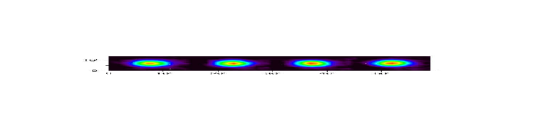
Figure 1: The beams of the $150\,$GHz array elements determined from observations of the CMB2 guiding quasar in the 2001 season. These images represent an average over the entire observation period and include any distortions due to changes in pointing or beamsize.

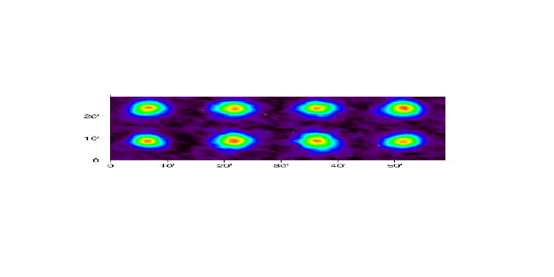
Figure 2: The beams of the $150\,$GHz array elements determined from observations of the guiding quasar in the CMB5 field. These images represent an average over the entire observation period and include any distortions due to changes in pointing or beamsize.

3.1 The Lead-Main-Trail Scan Strategy

During the CMB observations, the telescope tracks a position on the sky while the chopper sweeps the beams back and forth three degrees in azimuth. The motion of the chopper introduces systematic offsets into the data that must be treated in the analysis. As will be described in §3.3, the motion of the chopper causes the beams to move slightly ($\sim 2^{\prime}$) in elevation as they sweep in azimuth. This motion modulates the atmospheric emission and introduces an $\sim 5\,{\rm mK}(T_{air}/200\,{\rm K})(\tau/0.03)$ signal at an elevation of $45^{\circ}$, where $\tau$ is the zenith optical depth at $150\,$GHz. Although the telescope optics were designed to produce a stationary illumination pattern on the primary mirror, the illumination on the secondary mirror changes substantially with chopper angle. Snow accumulation or temperature differences on the secondary mirror will be modulated and contribute a second source systematic signal that varies with the chopper position.

The effects described above are collectively referred to as the chopper synchronous offset. Changes in the effective temperature of the atmosphere and optics throughout an observation can result in a time variation of this signal. In order to minimize the chopper synchronous offset, each field is observed in a rapid Lead-Main-Trail (LMT) sequence where the Main field is led and trailed by two identical Lead and Trail observations each with half the integration time of the main observation. The CMB power spectrum is derived from the differenced map, Main-(Lead+Trail)/2. If the LMT switching is performed faster than the time scale of any drift in the chopper synchronous offset, then the offset can be eliminated. Compared to the differencing of two equally weighted fields, the LMT observation further removes a linear drift in any chopper synchronous offset. In practice, the Lead field is tracked for 30 seconds; the telescope is moved $+3^{\circ}\sec\delta$ (in increasing RA) to track the Main field for 60 seconds; the telescope is moved another $+3^{\circ}\sec\delta$ to the Trail field for 30 seconds of integration. After completing the LMT cycle, the elevation of the telescope is decreased by $1^{\prime}$ and the process is repeated $\sim 100$ times to build up a continuous 2-dimensional map. The CMB2 and CMB5 fields actually consist of two largely overlapping sub-fields offset by $0.5^{\circ}{\rm sec}(\delta)$ in RA. The total observation time for each field is split roughly equally between the subfields which are referred to as CMB2a,b and CMB5a,b.

3.2 Data Cuts

In order to minimize the potential contamination of the data by systematic errors, we introduced a number of conservative data cuts. All 4 hour observations containing refrigerator temperatures higher than $250\,$mK cut from the data set due to their uncertain calibration. Cryogenics fills, refrigerator cycles, computer and telescope maintenance, and bad weather all limit observation time. Including galactic observations and calibrations, the effective observing efficiency was $\sim 60\%$ for the winter of 2002. The effects of cosmic ray interactions with the detectors were removed by discarding any chopper sweep containing a point varying from the mean of the raw $2.4\,$kHz data samples by $>6\sigma$. Due to the low filling factor of the micro-mesh detectors, this results in an insignificant loss of data. Before performing the LMT differencing, the data are examined for the presence of excessive chopper synchronous offsets that indicate the accumulation of snow on the mirrors. The offset level is bimodal between the two extremes and the amount of data cut depends only weakly on the cut level. Files with snow accumulation are discarded, resulting in a loss of approximately $40\%$ of the remaining data. The details of the cut level and amount of discarded data have no significant effect on the resulting maps or power spectrum. After implementing the data cuts described above, we retained $\sim 400$ hours of observation on CMB2 during July–August of 2001 and April of 2002. For CMB5 we retained $\sim 800$ hours of data gathered during April–July of 2002. As described in §4.1.3, we cut an additional $\sim 25\%$ of the remaining data that we determined to be corrupted by atmosphere induced correlations between array elements and adjacent scans.

3.3 Pointing

The Viper telescope pointing model is developed from observations of bright galactic sources, planets, and quasars. Daily observations of the compact galactic sources RCW38, RCW57 and MAT6a are used to monitor pointing offsets and check the pointing model. The pointing model contains terms for encoder offsets, collimation error, telescope flexure, and tilt of the AZ ring. When the telescope is pointed at the equator, the detector beams sweep out a strip of approximately constant elevation under the motion of the chopper. However, at the elevation at which the CMB observations are made, the beams sweep out arcs with amplitude of approximately $2\,^{\prime}$ across the $3^{\circ}$ chop. Observations of planets and galactic sources at a number of positions in the chopper throw have been used to characterize this effect. For each array element, we determine a pointing model that is a function of the elevation, azimuth, and chopper encoders. After applying the model, we find the RMS pointing error for the 2001 season to be $\sim 1.4^{\prime}$ in RA and $\sim 30^{\prime\prime}$ in declination. The majority of the spread in 2001 was due to a malfunctioning sensor of the chopper angle. After this sensor was replaced in January 2002, the pointing RMS was determined to be $\sim 20^{\prime\prime}$ in RA and $\sim 20^{\prime\prime}$ in declination. Due to early concerns about the accuracy of the pointing, we chose each CMB field to have a bright ( $\gtrsim 1\,$Jy at $5\,$GHz) quasar in the middle. In this way, we have an continuous monitor and independent check of the accuracy of the pointing.

3.4 Beams

High signal-to-noise maps of planets (Mars and Venus in July 2001, and Venus in September 2002) are used to accurately measure the beam patterns of the array elements. The measured maps were deconvolved with a constant temperature circular disk corresponding to the planet sizes (typically small compared to the beams), to determine the instantaneous beam parameters.

The coadded image of the guide quasar is used to determine the effective beamsizes at the center of the map and includes any smearing due to drifts in pointing that occur over the period in which the data are acquired. Focal plane maps for the array in both the 2001 and 2002 configurations are shown in Figures 1 and 2. In Table 1, we list the FWHM beam diameters derived from Gaussian fits to the quasar images for both years. These beam parameters were used in the analysis of CMB power spectrum. These results are consistent with the beamsizes measured on planets and the observed pointing RMS determined from repeated observations of galactic sources. Some of the beams in CMB5 quasar image appear to be slightly elongated in declination; we believe this to be due to the accumulation of frost on the dewar window during the 2002 observations. We estimate the uncertainty in the FWHM of the beams to be less than $3\%$.

Table 1: 150 GHz Beam Sizes

year	channel	${\rm FWHM}_{1}(^{\prime})$	${\rm FWHM}_{2}(^{\prime})$	P.A. (degree)
2001	C1	5.46	4.76	178
2001	C2	5.10	4.81	176
2001	C3	5.10	4.76	161
2001	C4	5.19	4.68	3
2002	D3	5.71	4.90	68
2002	D4	5.50	5.45	121
2002	D6	5.53	5.25	7
2002	D5	5.69	5.15	87
2002	B6	4.94	4.40	111
2002	B3	5.66	5.20	69
2002	B2	6.79	5.34	105
2002	B1	5.46	4.67	43

$\;\;\;\;\;\;\;\;\;\;\;\;\;\;\;\;\;\;\;\;\;\;\;\;\;\;\;\;\;\;\;\;\;\;\;\;\;\;\;\;\;\;\;\;\;\;\;\;\;\;\;\;\;\;\;\;\;\;\;\;\;\;\;\;{}^{a}$ Position angle from +RA, counterclockwise.

Due to aberrations in the telescope optics, the beam sizes increase slightly near the extremes of the chopper travel. This effect was characterized by mapping planets and galactic sources over a range of pointings offset in RA. The telescope beams were simulated with a ray-tracing package and the resulting aberrations were found to be consistent with the observations. The FWHM of the beams typically changes by $\sim 5\%$ over the entire chopper throw, and the throughputs are found to be conserved. The measured beams are found to be very close to symmetric Gaussians and we describe their shapes in terms of their small distortions. We parameterize the aberrations with three parameters: the distortions along RA, DEC, and an axis inclined at a 45^∘ position angle. When the distortions are small, all three parameters are small and can be treated with a perturbation analysis. In sections §4.2 and Appendix C, we describe how changes in the beam shape are treated in the computation of the power spectrum.

3.5 Calibration

The calibration of Acbar is described in detail by Runyan et al. (2002b); here we will present a brief summary. The planets Venus and Mars serve as the primary calibrators for the Acbar CMB observations. Due to the lack of a significant atmosphere and dielectric emission by the soil, the spectrum of Mars closely approximates that of a blackbody. The brightness temperature of Mars varies as a function of its distance from the sun with mean Heliocentric value of $\sim 206\,$K at $150\,$GHz. The FLUXES software package uses the brightness temperature adopted by Griffin et al. (1986) and an accurate ephemeris to compute instantaneous values for the Martian brightness temperature. Following Griffin & Orton (1993) we assign an overall uncertainty to the temperature of Mars of $5\%$. The brightness temperature of Venus is a function of frequency; following Weisstein (1996), we fit the brightness temperature of Venus with a linear fit to the published data. For the Acbar $150\,$GHz band, we adopt a brightness temperature of $297\pm{22}\,$K, close to the value of $294\pm 22\,$K reported by Ulich (1981) for a band centered about $150\,$GHz. From the South Pole, planets are only intermittently available for observation and are always at elevation $<30^{\circ}$. Observing them typically requires lowering a section of the groundshield and waiting for the sky to clear from the zenith to the horizon. For these reasons, it is impractical to use planets to regularly monitor the calibration of the instrument.

The HII region RCW38 is bright, compact, and has a declination similar to our CMB fields; therefore, it serves as an excellent secondary calibrator. The responsivities of the Acbar detectors are a function of the background loading and change slightly with elevation. Behind a small hole in the tertiary mirror, we have installed a chopped thermal load that produces a constant optical signal which is used to monitor the detector responsivity as a function of elevation. The difference in atmospheric attenuation between the planet and RCW38 observations must also be taken into account. Sky dips are used to measure the atmospheric opacity and correct for the effects of atmospheric attenuation. Because the emission from RCW38 is somewhat extended ($\sim 3^{\prime}$ FWHM) and beamsizes of Acbar differ slightly between the 2001 and 2002 observations, the integrated flux (to an angular radius of $8^{\prime}$) is used as our secondary calibration standard.

The integrated galactic source flux is given by

$$S_{I}=\int I_{P}(\nu)f(\nu)d\nu\frac{\int V_{G}d\Omega}{\int V_{P}d\Omega}\left(\frac{R_{P}}{R_{G}}\right)\left({\frac{e^{-\tau_{P}\csc(\theta_{P})}}{e^{-\tau_{G}\csc(\theta_{G})}}}\right)\,,$$ (1)

where $R_{P}$ and $R_{G}$ are the responsivities of of the detectors when observing the planet and galactic source, $V_{P}$ and $V_{G}$ are the measured voltages as a function of angular position, $\tau_{P}$ and $\tau_{G}$ are the zenith optical depths of the atmosphere, $\theta_{P}$ and $\theta_{G}$ are the elevations of the planet and galactic source observations, $I_{P}(\nu)$ is intensity of the planet, and $f(\nu)$ is the spectral response of the system as measured in the lab with a Fourier transform spectrometer as described by Runyan et al. (2002b). Both the Mars and Venus calibrations produce a consistent integrated flux for RCW38 at $150\,$GHz of $S_{I}=145\pm 7\,$Jy where the uncertainty reflects the scatter among the array elements and measurements. Including the uncertainty for the flux of the planets, the detector responsivities, and integral over solid angle, we find $S_{I}=145\pm 13\,$Jy which is dominated by the uncertainty in the planet brightness temperature.

We can now use RCW38 to monitor the calibration of the instrument and transfer the calibration to our CMB observations. Observations of RCW38 are scheduled to bracket each $\sim 5$-hour CMB observation. The zenith optical depth at $350\,\mu$m is measured every 15 minutes with a tipping radiometer (Peterson et al. 2002) and is extrapolated to $150\,$GHz using the observed scaling between the measured Acbar $150\,$GHz opacity and $350\,\mu$m tipper optical depths. After correcting for varying atmospheric attenuation, the integrated RCW38 flux is found to be constant over all observations with an RMS scatter of $\lesssim 4\%$. Because both of the CMB fields are observed at elevations similar to RCW38, the responsivity can be considered to be constant. Although small, the difference in optical depth between the RCW38 calibration and the CMB field must still be taken into account. The conversion from observed bolometer voltage signals to CMB temperature differences is given by

$$\frac{dT_{CMB}}{dV_{bolo}}=\frac{S_{I}}{\int\frac{dB(\nu)}{dT_{CMB}}f(\nu)d\nu\int{V_{G}\,d\Omega}}\left({\frac{e^{-\tau_{G}\csc(\theta_{G})}}{e^{-\tau_{CMB}\csc(\theta_{CMB})}}}\right)\,,$$ (2)

where $B(\nu)$ is the intensity of a $2.73\,$K CMB blackbody, and $\theta_{CMB}$ is the elevation of the CMB observation.

Given the stability of the frequent RCW38 observations, the statistical accuracy of the calibration transfer from RCW38 to the CMB fields is quite good. The uncertainty in the calibration is a combination of the uncertainty of the planet brightness temperatures, beamsize measurements, spectroscopy, and accuracy of the calibration transfer. Assuming a common overall uncertainty in the calibration of Mars and Venus, we estimate the uncertainty in the temperature calibration of the observed CMB anisotropy to be $\pm 10\%$.

4 Analysis

Algorithms for the analysis of total power CMB data are well developed and have been tested on balloon-borne experiments (Netterfield et al. 2002; Lee et al. 2001). However, the ground-based Acbar experiment is subject to constraints which require significant departures from the standard analysis algorithms. In this Section, we outline the Acbar analysis and highlight its unique features.

4.1 Maximum Likelihood Map and Noise Weighted Coadded Map

The first step of the analysis is to produce a map from the timestream data. Suppose $d_{\alpha}\;$($\alpha=1..n_{t}$) are $n_{t}$ time-ordered measurements of CMB temperature. This vector can be separated into the noise component $n_{\alpha}$ and the signal component $\sum_{j}A_{\alpha j}T^{0}_{j}$, such that $d_{\alpha}=n_{\alpha}+\sum_{j}A_{\alpha j}T^{0}_{j}$, or in matrix representation, ${\bf d}={\bf n}+{\bf AT^{0}}$. Here $T^{0}_{j}$ ($j=1..n_{p}$) are the CMB temperatures on each sky pixel $j$, after being convolved with the “beam”, or the experimental response function. For these observations, this will be a Lead[-1] Main[+2] Trail[-1] three point beam function. ${\bf A}$ is the $n_{t}\times n_{p}$ pointing matrix where $A_{\alpha j}=1$ if $\alpha\in j$ (measurement $\alpha$ corresponds to sky pixel $j$); and $A_{\alpha j}=0$ otherwise. If ${\bf n}\gg{\bf AT^{0}}$ (as is the case for the Acbar data), the time stream correlation can be determined from the data itself; $\langle n_{\alpha}n_{\beta}\rangle\equiv N_{\alpha\beta}\sim\langle d_{\alpha}d_{\beta}\rangle$.

In general, a map ${{\bf T}}$ is produced from a linear combination of the timestream ${\bf d}$;

$${{\bf T}}\equiv{\bf Ld},$$

where ${\bf L}$ is a $n_{p}\times n_{t}$ coefficient matrix. The map “pixel” space correlation matrix is given by

$$\langle{{\bf T}}\;{{\bf T}}^{t}\rangle={\bf L}\langle{\bf d}{\bf d}^{t}\rangle{\bf L}^{t}={\bf L}{\bf N}{\bf L}^{t}+{\bf L}{\bf A}\langle{\bf T^{0}}{\bf T^{0}}^{t}\rangle{\bf A}^{t}{\bf L}^{t}\\$$

$$\equiv{\bf C}_{N}+{{\bf C}}_{T}.$$ (3)

4.1.1 Maximum Likelihood Map

In balloon-borne or satellite experiments, the matrix ${\bf L}$ is usually taken to be

$${\bf L}={\bf L_{m}}=({\bf A}^{t}{\bf N}^{-1}{\bf A})^{-1}{\bf A}^{t}{\bf N}^{-1},$$ (4)

and the resulting map ${{\bf T}}_{m}$ is the maximum likelihood map. Using eq. [3], the correlation matrix for the maximum likelihood map can be derived:

$$\langle{{\bf T}}_{m}\;{{\bf T}}_{m}^{t}\rangle=({\bf A}^{t}{\bf N}^{-1}{\bf A})^{-1}+\langle{\bf T^{0}}{\bf T^{0}}^{t}\rangle.$$ (5)

It was shown by several authors (Tegmark 1997; Ferreira & Jaffe 2000) that a maximum likelihood map is not only a good visual representation of the data, but also a lossless way to compress CMB information; the power spectra derived from the map and directly from the timestream will have the same uncertainty.

However, for a ground based experiment like Acbar, the vertical gradient in atmosphere emission restricts the observation to constant elevation strips. Furthermore, the special location of the Viper telescope ($\sim 1$ km from the geographic South Pole) results in maps with little cross-linking in declination. In addition, the large angular scale structure in the timestream is dominated by atmospheric fluctuations. The lack of cross-linking, and the need to remove large angular scale ($\gtrsim 1^{\circ}$) sky noise results in numerical problems in the computation of the maximum likelihood map and an alternative analysis is required.

4.1.2 Demodulation Analysis

One can select certain linear combinations of ${\bf d}$ which are believed to be free from sky noise contamination. In this case, the coefficient matrix ${\bf L}$ is formed by rows of sky “modulation” patterns, which are usually taken to be edge-tapered sinusoidal functions. This method is known as the demodulation analysis, and has been used successfully by several ground based CMB experiments (Netterfield et al. 1997; Miller et al. 1999; Peterson et al. 2000).

One of the disadvantages of demodulation analysis is that the choice of modulation patterns is arbitrary, and could result in the loss of useful information. In other words, the choice of ${\bf L}$ could result in a power spectrum with uncertainties considerably larger than the those found from the maximum likelihood map (Tegmark 1997). Furthermore, the modulated data, or the “map” ${\bf Ld}$, has little to do with the actual CMB temperature distribution on the sky, making it difficult to treat foregrounds and test for systematic errors. We performed a demodulation analysis of the Acbar data presented in this paper as an early check of our analysis technique. The resulting power spectrum was found to be roughly consistent with that presented here, although with somewhat larger uncertainties.

4.1.3 Noise Weighted Coadded Map

Due to time varying atmospheric emission, there are large signals in the data timestream. These signals are easy to remove from the timestream, however, they cannot be simply removed from the final map. Therefore, it is essential that the corrupted modes corresponding to the atmosphere be removed before the data are coadded to form a map. We propose to use the cleaned noise-weighted coadded map as an intermediate analysis step. The operation of the “corrupted mode projection” matrix ${\bf\Pi}$ on the timestream ${\bf d}$ projects out the undesired modes, resulting in the cleaned timestream data ${\tilde{\bf d}}\equiv{\bf\Pi d}$. We take ${\bf\Pi}$ to be a block-diagonal matrix, where the length of each block corresponds to a chopper sweep. Each block removes certain modes in each data strip. If ${\bf U}$ consists of $m$ columns of linearly independent undesired modes, the projection matrix block can be defined as ${\bf\Pi_{b}}\equiv{\bf I}-{\bf U}({\bf U}^{t}{\bf U})^{-1}{\bf U}^{t}$ (Tegmark 1997). It is easy to see ${\bf\Pi_{b}}{\bf U}=0$, and ${\bf\Pi_{b}}^{t}={\bf\Pi_{b}}$.

With the corrupted modes removed, we can define the cleaned noise weighted coadded map as

$${\tilde{T}}_{i}=\lambda_{i}\sum_{\alpha\in i}\omega_{\alpha}\tilde{d}_{\alpha}.$$

$\lambda_{i}\omega_{\alpha}$ is the “weight” associated with measurement $\alpha$ on pixel $i$. The normalization condition requires that

$$\lambda_{i}\sum_{\alpha\in i}\omega_{\alpha}=1.$$

The cleaned map can be represented as a linear combination of the raw timestream;

$${\tilde{\bf T}}\equiv{\tilde{\bf L}}{\bf d},\;\;\;{\rm where}\;\;\;{\tilde{\bf L}}\equiv{\bf\Lambda}{\bf A}^{t}{\bf\Omega}{\bf\Pi}.$$ (6)

Here ${\bf\Omega}$ and ${\bf\Lambda}$ are diagonal matrices,

$$\Omega_{\alpha\beta}=\delta_{\alpha\beta}\omega_{\alpha},\;\;\;\;\Lambda_{ij}=\delta_{ij}\lambda_{i}.$$

In practice, each sample $\alpha$ is weighted on its inverse variance after the projection of the corrupted modes,

$$\omega_{\alpha}=\frac{1}{\sigma_{\alpha}^{2}},\;\;\;\;\;\sigma_{\alpha}^{2}=\sum_{\beta\gamma}\Pi_{\alpha\beta}N_{\beta\gamma}\Pi_{\alpha\gamma}.$$

To clarify the relation between the maximum likelihood map and the noise weighted coadded map, we investigate the special case where the noise ${\bf N}$ is diagonal ($N_{\alpha\beta}=\delta_{\alpha\beta}\sigma_{\alpha}^{2}$) and no modes are projected out (${\bf\Pi}={\bf I}$),

$${\tilde{T}}_{i}=\sum_{\alpha}{\tilde{L}}_{i\alpha}d_{\alpha}=\frac{\sum_{\alpha}d_{\alpha}A_{\alpha i}/\sigma_{\alpha}^{2}}{\sum_{\gamma}A_{\gamma i}/\sigma_{\gamma}^{2}}$$

$$=\left[({\bf A}^{t}{\bf N}^{-1}{\bf A})^{-1}{\bf A}^{t}{\bf N}^{-1}{\bf d}\right]_{i}.$$

In this case, ${\tilde{\bf T}}$ is identical to the lossless maximum likelihood map. In general, ${\tilde{\bf T}}$ will not be lossless; however, if the off diagonal terms of ${\bf N}$ are small, ${\tilde{\bf T}}$ will approach the lossless map. This is the case for Acbar.

From eq. [4], and $\langle{\bf d}\rangle=\langle{\bf n}\rangle+{\bf AT^{0}}={\bf AT^{0}}$, it is easy to show that the maximum likelihood map is an unbiased estimate of the CMB sky temperature: $\langle{{\bf T}}_{m}\rangle={\bf T^{0}}$. However, this is not the case for ${\tilde{\bf T}}$, since

$$\langle{\tilde{\bf T}}\rangle={\bf K}{\bf T^{0}}\neq{\bf T^{0}};\;\;{\rm where}\;\;{\bf K}\equiv{\tilde{\bf L}}{\bf A}.$$ (7)

Therefore the transformation of the theory matrix ${{\bf C}}_{T}={\bf K}\langle{\bf T^{0}T^{0t}}\rangle{\bf K}^{t}$ in eq. [3] is nontrivial and has to be calculated in the coadding process. Explicitly,

$$K_{ij}=\lambda_{i}\!\!\sum_{\alpha\in i;\,\beta\in j}\!\!\omega_{\alpha}\Pi_{\alpha\beta}\;$$ (8)

is the transformation matrix between the sky and our “map” space. Hereafter we drop the tilde and simply write $\tilde{\bf T}$ as ${\bf T}$. The untransformed sky temperature is denoted by ${\bf T^{0}}$.

Note that the contaminated mode projection matrix ${\bf\Pi}$ is completely arbitrary and can be made to adapt to the conditions of a given observation. We take ${\bf\Pi}$ to be block-diagonal, each block ${\bf\Pi_{b}}$ removes polynomial functions of certain orders in each chopper sweep. The order of the polynomial to be removed depends on the atmospheric conditions during the observation. In this way, data corrupted by atmospheric emission on large angular scales can still contribute to the determination of the small scale power. Quantitatively, the polynomial order is chosen to be the lowest such that the residual correlation between sweeps in the “stare” (data strip of constant DEC pointing) is less than $5\%$. If after removing a 10th order polynomial a residual correlation greater than $5\%$ remains, the data are discarded. To avoid bias in noise estimation the order of the polynomial to be removed is constant over 20 minutes duration. The correction matrix ${\bf K}$ for the map is built by coadding the correction matrices for the individual scans with the appropriate noise weighting. The resulting correction matrix ${\bf K}$ was used in a series of Monte Carlo simulations to show the band-powers themselves are unbiased by the adaptive removal of contaminated modes.

4.2 Noise Matrix

The precise determination of the noise correlation properties of the data is a non-trivial task for high-sensitivity ground based experiments. From eqs.[3,6], the calculation of noise correlation matrix $C_{N}$ for ${\bf T}$ is straightforward once the timestream noise ${\bf N}$ is known:

$${C}_{N\{ij\}}=\lambda_{i}\lambda_{j}\!\!\sum_{\alpha\in i;\;\;\beta\in j}\!\!\omega_{\alpha}\omega_{\beta}\sum_{\gamma\delta}\Pi_{\alpha\gamma}N_{\gamma\delta}\Pi_{\beta\delta}\;,$$ (9)

or in matrix notation,

$${{\bf C}}_{N}={\bf\Lambda}{\bf A}^{t}{\bf\Omega}{\bf\Pi}{\bf N}{\bf\Pi}^{t}{\bf\Omega}{\bf A}{\bf\Lambda}.$$

This is just a weighted average of ${\bf\Pi}{\bf N}{\bf\Pi}^{t}$. However, since the noise in the timestream is far from stationary, the determination of ${\bf N}$ requires careful treatment (see Appendix A). We are confident that the noise correlation for the data presented here has been determined to to better than $5\%$.

4.3 Theory Matrix

The observed CMB temperature $T^{\prime}(\theta,\phi)$ is the convolution of the real temperature $T(\theta,\phi)$ with the experimental response function $B(\theta,\phi)$. For a LMT subtracted experiment, $B(\theta,\phi)$ is the convolution of the beam $B_{0}(\theta,\phi)$ with the beam-switching pattern

$$\Xi({\hat{\bf r}})=\delta({\hat{\bf r}})-[\delta({\hat{\bf r}}-{\hat{\bf r}}_{1})+\delta({\hat{\bf r}}-{\hat{\bf r}}_{2})]/2,$$ (10)

where $\delta$’s are the Dirac $\delta$- functions. For Acbar, ${\hat{\bf r}}_{1}=(0,\Delta\phi)$ and ${\hat{\bf r}}_{2}=(0,-\Delta\phi)$ , where $\Delta\phi=3^{\circ}\csc\theta$. The Gaussian temperature anisotropy can be described by the angular power spectrum $C_{\ell}$, or the mean square of the multipole moments: $C_{\ell}=\langle a_{\ell m}^{*}a_{\ell m}\rangle\;.$ When the observations are restricted to small fractions of the celestial sphere, the spherical harmonic series can be approximated by two dimensional Fourier series. In this limit, the 2-D power spectrum density (PSD) is the product of $|{\cal B}({\bf k}={\bf\ell}/2\pi)|^{2}$ and $C_{\ell}$, where ${\cal B}$ is the Fourier transform of $B$. (Saez et al. 1996). For a given power spectrum and observational response function, the theory matrix gives the temperature correlation between pixel pairs in the map. Since the PSD and the autocorrelation function (ACF) form a Fourier transform pair, the theory matrix can be calculated efficiently with Fast Fourier transform (FFT) technique.

However, the noise weighted coadded map defined in eq.[6] combines sky temperatures measured by channels with different beam sizes at different chopper positions. Therefore, each pixel has different beam parameters, and strictly speaking, the FFT algorithm is not applicable. The straightforward calculation of the theory matrix and its derivatives with respect to band-powers involves a computationally expensive four dimensional integral for each pixel pair. A common way to deal with this problem is to average the beam for the entire map, and generate the theory matrix from the average beam (Wu et al. 2001).

We have developed an alternative approach that employs a semi-analytic correction formula to treat the variation of beam sizes in the map. The beams for each measurement are coadded accounting for the position of each sample and allowing for changes in the beamshape. Different pixel pairs then receive an individual correction to the overall FFT result, depending on the pixel-beam parameters. The full derivation of this technique is given in Appendix C. Due to the small changes in beamshape ($\sim 5\%$ FWHM), the effect of the beamshape correction is small and does not result in significant changes in the measured power spectrum.

4.4 Power Spectrum Estimation

The first step in the estimation of the power spectrum is the determination of a function describing the likelihood that the data are described by a given model. Assuming Gaussianity, the likelihood function is

$${\cal L}\propto|{\bf C}|^{-1/2}\exp\left[-\frac{1}{2}{\bf T^{t}C^{-1}T}\right],$$ (11)

where ${\bf C}={\bf C}_{T}+{\bf C}_{N}$. Once ${{\bf C}}_{N}={\tilde{\bf L}}{\bf N}\tilde{\bf L}^{t}$, ${\bf K}={\tilde{\bf L}}{\bf A}$, and ${{\bf T}}={\tilde{\bf L}}{\bf d}$ are calculated from the time stream, the anisotropy power spectrum can be readily estimated by the standard maximum likelihood method. The only difference is the replacement of ${\bf C}_{T}$ with ${\bf K}{\bf C}_{T}{\bf K}^{t}$.

4.4.1 Signal-to-Noise Eigenmodes And Foreground Removal

Following Bunn & White (1997) and Bond et al. (1998), the data are further compressed using signal-to-noise eigenmode truncation (Karhunen-Lo’ eve transformation). With slight modifications, this can be done simultaneously with the removal of foreground templates. Our foreground removal method is conceptually the same as the constraint matrix formalism (Bond et al. 1998; Halverson et al. 2002), or the pseudo-inversion of Tegmark (1997). The idea is to replace the inverse of Hermitian square root or Cholesky decomposition (${\bf C}_{N}^{-1/2}$) in eq.[A4] of Bond et al. (1998) with a non-square “whitening” matrix. This procedure is described in detail in Appendix D. The foreground modes removed from the CMB2 and CMB5 fields are described in § 6 and listed in Tables 3 and 4.

4.4.2 Iterative Quadratic Approach to Maximum Likelihood Band-Power

The anisotropy power spectrum is parameterized by the band-power ${\bf q}$, where

$$D_{\ell}\equiv\frac{\ell(\ell+1)}{2\pi}C_{\ell}=\sum_{B}q_{B}\chi_{B\ell}.$$ (12)

A convenient choice of $\chi_{B\ell}$ are “tophat” functions, i.e., $\chi_{B\ell}=1$ for $\ell\in B$; and $\chi_{B\ell}=0$ for $\ell\not\in B$. The maximum likelihood ${q_{B}}$s are estimated iteratively using the quadratic iteration method (Bond et al. 1998). Near the extrema, the log of the likelihood function can be approximated by a multidimensional quadratic function. The true maximum of the original $\cal L$ can then be found by an iterative process:

$${q_{B}}^{n+1}={q_{B}}^{n}+\rho\frac{1}{2}({\bf F}^{-1}{\bf y})_{B},$$ (13)

where

$$y_{B}=({{\bf T}}^{t}{\bf C}^{-1}{{\bf C}}_{T,B}{\bf C}^{-1}{{\bf T}})-{\rm Tr}({\bf C}^{-1}{{\bf C}}_{T,B}),$$ (14)

and

$$F_{BB^{\prime}}=\frac{1}{2}{\rm Tr}({\bf C}^{-1}{{\bf C}}_{T,B}{\bf C}^{-1}{{\bf C}}_{T,B^{\prime}}).$$ (15)

$C_{T,B}$ is the partial derivative of $C_{T}$ with respect to $q_{B}$. With eq. [12], it is easy to see

$$C_{T,B}=\sum_{\ell}\frac{\partial C_{T}}{\partial D_{\ell}}\chi_{B\ell}\,.$$ (16)

The relaxation factor $\rho$ is a numerical constant between $0$ and $1$. The converged power spectrum is independent of $\rho$, however setting $\rho<1$ prevents the estimated $q_{B}$ from “overshooting” and wandering to some local extrema. Empirically, $\rho=0.5$ worked very well, and the $q_{B}$’s converged after a few iterations.

4.4.3 Decorrelated Band-Powers

Due to the nature of the experiment (partial sky coverage, correlated noise in the timestream, etc.), the band-power values are not independent. The correlations between them are given by the inverse of the Fisher matrix (eq. [15]). To get the correct uncertainty estimate for a band-power value we either need to marginalize over all the other bands, or perform a linear transformation to decorrelate the data points. We chose to decorrelate the data points to maintain as much information as possible. The decorrelation matrices are not unique: our choice is the Hermitian square root of Fisher matrix, because it is localized and symmetric (Tegmark 1997). In the new basis, the local likelihood function is in canonical form.

4.4.4 Shape of the Likelihood Function

It was pointed out by Bond et al. (2000) that an offset log-normal function is a much better approximation to the likelihood function than a quadratic one. Failing to account for this could lead to serious misinterpretation of an experimental result, a most notable example being the quadrupole moment measured by COBE. In the decorrelated basis, the likelihood function near the maximum ($q_{B}={\overline{q}}_{B}$) can be approximated by an offset log-normal function

$$\ln{\cal L}({\bf q})=\ln{\cal L}(\overline{{\bf q}})-\frac{1}{2}\sum\limits_{B}\frac{(Z_{B}-\overline{Z}_{B})^{2}}{\sigma_{B}^{2}}e^{2{\overline{Z}}_{B}},$$ (17)

where the offset log-normal parameters ${\bf Z}$ are defined as

$$Z_{B}=\ln{(q_{B}+x_{B})}.$$ (18)

Even to the quadratic order, the Fisher matrix is only an approximation to the curvature matrix of the likelihood function near the extrema. To examine the real shape of the likelihood function, we explicitly fit the curvature $\sigma_{B}$ and log-normal offset $x_{B}$ and compared the results with the Fisher matrix (now diagonal) and the offsets suggested by Bond et al. (2000) (see their eq. [28]). In general we found very good agreement. In a few bands, however, the uncertainty indicated by the true likelihood function is $\sim 15\%$ larger than that derived from the Fisher matrix. The uncertainty and log-normal offsets reported in this paper are determined from fits to the likelihood function.

4.4.5 Window Functions

Our goal is to produce a CMB power spectrum that can be used to constrain cosmological models. Window functions are used to convert a given model power spectrum to quantities directly comparable to the band-power measurements of the experiment. A window function $W_{B\ell}$ for band “$B$” should have the following property:

$$\langle q_{B}\rangle=\sum_{\ell}(W_{B\ell}/\ell)D_{\ell}\,,$$

where $q_{B}$ is the experimental band-power measurement. Knox (1999) derived the appropriate window function for the band-power quadratic estimator (Tegmark 1997),

$$W_{B\ell}/\ell=\frac{1}{2}\sum_{B^{\prime}}(F^{-1})_{BB^{\prime}}{\rm Tr}\left(\frac{\partial C_{T}}{\partial D_{\ell}}C^{-1}C_{T,B^{\prime}}C^{-1}\right)\,.$$

This form of window function has been used in several other experiments (Halverson 2002; Pryke et al. 2002; Meyers et al. 2002), and should serve as a good approximation for maximum likelihood band-power. Making use of eqs. [15][16], it can be shown that the pre-decorrelation window functions satisfy the following normalization condition,

$$\sum_{\ell}\chi_{B\ell}W_{B^{\prime}\ell}/\ell=\delta_{BB^{\prime}}\,.$$ (19)

In Section §4.4.3, we described the computation of a set of decorrelated band-powers from the Fisher matrix of the raw band-powers. This same linear transformation is applied to the window functions to produce a set of decorrelated window functions.

It is not necessary to calculate the window functions for all $\ell$. However, we would like to sub-divide the $q_{B}$ bands into bins with finer $\ell$ space resolution than the $q_{B}$ themselves. Otherwise in order to satisfy the normalization condition eq. [19], the pre-decorrelation window function reduces to a Kronecker-$\delta$ in band index “$B$”, or the tophat function given by $\chi_{B\ell}$. This is a reasonable approximation for experiments like BOOMERANG where the sky coverage, and therefore intrinsic $\ell$ resolution, is large enough to resolve all the structures in the power spectrum. For Acbar, the $\ell$ resolution of the experiment is comparable to the expected structure in $D_{\ell}$ and it is essential to precisely characterize the dependence of each band power on the details of the power spectrum. The decorrelated window functions shown in Figure 3 were calculated with a resolution in $\ell$ space of $\Delta\ell=30$. The first window function has significant oscillations with $\Delta\ell\sim 110$. This appears to be an result of the close spacing of the fields in the LMT subtraction. For sufficiently smooth theoretical models these oscillations will average to a mean value, however, the exact dependence of the first band power on arbitrary input models could be complex. Numerical tabulations of the window functions are available on the Acbar public web site.

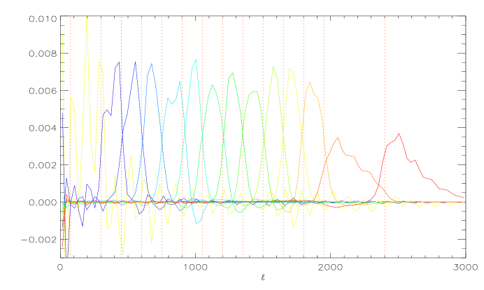
Figure 3: The window functions ($W_{B\ell}/\ell$) for the decorrelated Acbar band powers. The vertical lines show the band boundaries. Numerical tabulations of these functions are given on the Acbar website.

4.4.6 Monte Carlo Simulations

In order to test our analysis technique, we performed 300 Monte Carlo realizations of CMB2 and CMB5 maps that are consistent with our observed noise statistics and the same underlying $\Lambda$CDM model. These maps were processed exactly as the real data, including using the same projection of corrupted modes, in order to test the ability of our pipeline to accurately determine the input CMB power spectrum. A quadratic estimator technique (Tegmark 1997) is used to rapidly determine the power spectrum for each of 300 realizations. In Figure 4, we show the resulting average power spectrum overlaid on the input model. It is clear that the input model is recovered without bias, even in the low $\ell$ bins that are sensitive to the angular scales on which the mode removal is occurring.

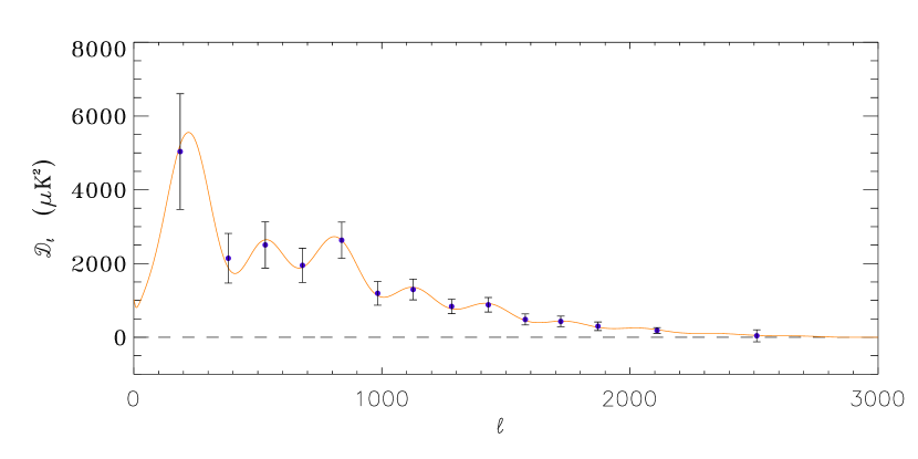
Figure 4: The results of 300 Monte Carlo runs using the measured Acbar noise correlation. The solid line is the input fiducial $\Lambda$CDM model. It is clear that the analysis method accurately reproduces the input power spectrum.

5 Results

5.1 Maps

Using the technique described in § 4.1.3, the LMT subtracted data are combined to form the noise weighted coadded maps shown in Figures 5 and 6. Due to computational limitations, we choose the map pixelization to be $2.5^{\prime}$. This is a compromise that allows us to recover the power spectrum with minimal loss of information while keeping the time and memory requirements reasonable for a single 16 processor, 64 GB RAM node of the National Energy Scientific Computing (NERSC) IBM SP computer. These maps have had the two guide quasars and one additional detected radio source (Pictor A) removed; black pixels mark the effected areas. Pictor A is observed to be extended and we remove a larger number of pixels around the position of this source. These maps have not yet had the undetected PMN source catalog and IRAS dust templates projected out; however, no other significant sources remain. For the purposes of presentation, we have smoothed the pixelized map with a $4.5^{\prime}$ FWHM Gaussian beam. The lower panels in Figures 5 and 6 show the RMS noise in the LMT difference maps as a function of position. Due to differences in map coverage, the noise varies across the map; in the central region, the RMS noise per $5^{\prime}$ beam is found to be $17\,\mu$K and $8\,\mu$K for CMB2 and CMB5 respectively. On degree angular scales, the S/N in the center of the CMB5 map approaches 100.

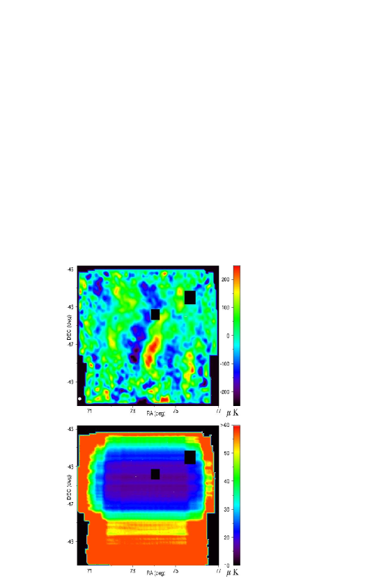
Figure 5: The top panel shows the LMT differenced, atmospheric mode removed, noise weighted, coadded map for the CMB2 field. The guide quasar and radio source Pictor-A have been replace with black pixels. The small white circle in the lower left hand corner of the map represents the FWHM of the average array element beamsize as determined from the coadded quasar image. The predominance of extended structure in the vertical direction is because the extended horizontal structure has been projected out in the atmospheric mode removal. The lower panel shows the noise in the LMT difference map as a function of position.

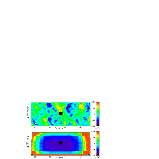
Figure 6: The same maps as shown in Figure 5, but for the CMB5 field. The signal-to-noise in the center of this map for degree-scale fluctuations approaches 100.

5.2 Band-Powers

After projecting out the PMN catalog and dust templates, the formalism described in § 4.4 is used to to determine the angular power spectrum. The resulting band-powers are correlated at the $\sim 20\%$ level before they are decorrelated. The decorrelated band power values are plotted in Figure 7 with a fiducial $\Lambda$CDM model; these same results are listed in Table 2. The corresponding decorrelated band-power window functions are plotted in Figure 3. Before decorrelation, the window functions are typically anticorrelated to those of adjacent bands at a level of $\sim 15\%$. After decorrelation, the anticorrelations decrease substantially. The decorrelated band-powers and tabulated window functions are available on the Acbar experiment public website.

Table 2: Joint Likelihood Bandpowers

$\ell$ range	$\ell_{-}$	$\ell_{+}$	$\ell_{\rm eff}$	$q$ ($\mu{\rm K}^{2}$)	$\sigma$ ($\mu{\rm K}^{2}$)	x ($\mu{\rm K}^{2}$)
75-300			187	6767	1323	-45
300-450	307	459	389	2874	605	-501
450-600	462	602	536	2716	498	-328
600-750	615	744	678	2222	360	-391
750-900	751	928	842	2300	355	-154
900-750	921	1048	986	798	153	-76
1050-1200	1040	1214	1128	1305	208	-10
1200-1350	1207	1352	1279	583	130	36
1350-1500	1338	1513	1426	628	134	111
1500-1650	1510	1649	1580	351	110	160
1650-1800	1648	1785	1716	248	99	149
1800-1950	1782	1953	1866	361	132	277
1950-2400	1946	2227	2081	337	109	557
2400-3000	2377	2651	2507	307	275	1888

Table 3: CMB2 Foreground modes

	RA	DEC	Degrees of Freedom
PMN J0455-4616	$04^{h}55^{m}51^{s}$	$-46^{\circ}15^{\prime}59^{\prime\prime}$	49
Pictor A	$05^{h}19^{m}50^{s}$	$-45^{\circ}46^{\prime}44^{\prime\prime}$	81
SFD dust map	-	-	1
Other PMN sources	-	-	102

Table 4: CMB5 Foreground modes

	RA	DEC	Degrees of Freedom
PMN J0253-5441	$02^{h}53^{m}29^{s}$	$-54^{\circ}41^{\prime}51^{\prime\prime}$	49
SFD dust map	-	-	1
Other PMN sources	-	-	68

6 Foregrounds

Sources of foreground emission have the potential to contaminate the measured CMB power spectrum. Multifrequency observations can be used create templates for some foregrounds and remove their effect from the power spectrum. At our observation frequencies, thermal emission from galactic dust, extragalactic radio sources, dusty protogalaxies, and the Sunyaev-Zel’dovich effect are all potential sources of foreground emission (Tegmark & et al. 1999).

The observed CMB fields were chosen to lie in a region of minimal dust contrast near the southern galactic pole. Templates for the dust emission are determined by performing a LMT difference on the IRAS/DIRBE maps published by Schlegel et al. (1998). The emission is extrapolated to $150\,$GHz, using the scaling of Finkbeiner et al. (1999). From this analysis, we expect contributions to the observed temperature anisotropy power in the differenced maps of $9\,\mu{\rm K}^{2}$ and $70\,\mu{\rm K}^{2}$ for CMB2 and CMB5 respectively. This power is dominated by structure on the scale of the map and decreases on smaller angular scales ($\propto 1/\ell$). The contribution of dust to the observed power is therefore expected to be completely negligible across the entire Acbar angular power spectrum. Projecting out dust emission using the IRAS/DIRBE template results in the loss of only one degree of freedom and has no significant effect on the resulting power spectrum.

Extragalactic Radio sources are another potential source of foreground confusion. By comparing the positions of known radio sources from the PMN $5.0\,$ GHz survey (Wright et al. 1994) with the CMB maps, we have detected 3 radio sources with significance greater than $3\sigma$. Two of these are the guiding quasars deliberately selected to lie in the center of the observed fields. In Tables 3 and 4, we list the coordinates of these sources and the number of pixels removed to clean them from the maps. It is possible that many PMN sources lie just below the threshold of detection and therefore contribute statistically to the observed power spectrum. We created templates which include all 170 PMN point sources in the CMB field with fluxes greater that $40\,$mJy at $5.0\,$GHz and use it to project out any possible contribution to the measured power spectrum. In Figure 7, we show the CMB angular power spectrum with and without the projection of the undetected point sources and the dust templates. Unless stated otherwise, all results in this paper are found with an analysis that removes these source templates.

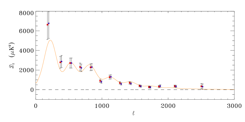
Figure 7: The CMB angular power spectrum with (circle) and without (square) the projection of templates for PMN radio point sources and thermal dust. Removing these sources of foreground emission has no significant effect on the measured power spectrum. The bandpower values and confidence intervals for the foreground projected power spectrum are listed in Table 2.

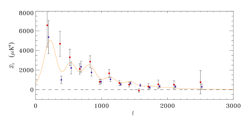
Figure 8: The CMB angular power spectrum derived from CMB2 (square) and CMB5 (circle) field.

It is also possible that dusty protogalaxies could contribute to the observed CMB signal. Unlike the radio sources, we have no template for the positions of these objects. Blain et al. (1998) have estimated the contribution of dusty protogalaxies to measurements of CMB anisotropy and predict a contribution to the $150\,$GHz power spectra of $(\Delta T)^{2}\sim 10\,(\ell/2500)^{2}\,\mu{\rm K}^{2}$. Therefore, dusty protogalaxies are not expected to contribute significant signal to the observed CMB anisotropy.

The most likely candidate for contamination of the observed Acbar power spectrum is the Sunyaev-Zel’dovich (SZE) effect in distant clusters of galaxies. Analytic models and numerical simulations generally predict a SZE power spectrum with a broad peak at angular scales corresponding to $\ell\sim 10^{4}$ (White et al. 2002). Deep observations with the Cosmic Background Imager (CBI), observing in a frequency band of $26-36\,$GHz and at angular scales corresponding to $\ell=2000-3500$, have reported a significant detection of excess power $(\Delta T)^{2}=506^{+116}_{-149}\,\mu{\rm K}^{2}$ (Mason et al. 2002). Interpreting this power as the SZE leads to a value for the RMS mass fluctuations inside spheres of $8\,h^{-1}$Mpc of $\sigma_{8}\sim 1.0$, close to the upper limits allowed by observations of the matter power spectra (Bond et al. 2002; Komatsu & Seljak 2002). Similar observations with the Berkeley Illinois Maryland Association (BIMA) array at a frequency of $28.5\,$GHz and on angular scales closer to the expected peak in the SZE power spectrum $(\ell_{\rm eff}=6864)$ also find excess power, $(\Delta T)^{2}=202^{+139}_{-135}\,\mu{\rm K}^{2}$ (Dawson et al. 2002) that is marginally consistent with the results reported by CBI. If these signals are in fact due to the SZE, we can use the spectral dependence of the SZE to predict the contribution to the Acbar power spectrum. Neglecting relativistic corrections, the observed change in CMB temperature in the direction of a galaxy cluster with Comptonization $y$ is given by

$$\Delta T=T_{CMB}\,y\left(\frac{x(e^{x}+1)}{e^{x}-1}-4\right)\,,$$ (20)

where $x=h\nu/kT_{CMB}$. Therefore, the CMB temperature anisotropy power due to the SZE should be a factor $\Delta T^{2}(150\,{\rm GHz})/\Delta T^{2}(30\,{\rm GHz})=0.238$ smaller for Acbar than was found by CBI and BIMA. In Figure 7 we show the Acbar and CBI power spectra plotted on top of a $\Lambda$CDM power spectrum. The marginal detection of excess power in the last Acbar band-power is consistent with the extrapolation of the CBI excess power to $150\,$GHz if the signal is due to SZE. However, due to the large uncertainty on this point, the Acbar results are also consistent with the origin of the CBI excess being due to CMB anisotropy from local structure and non-standard inflationary models Cooray & Melchiorri (2002); Griffiths et al. (2002) or a new population of faint radio point sources.

7 Systematic Tests

7.1 Gaussianity

The derivation of the band-power ${\bf q}$ is based on the assumption that the signal is Gaussian distributed. This assumption is tested by examining the distribution of signal-to-noise eigenmodes ${\bf T}_{s}$ (Appendix D). After the maximum likelihood band-powers are found, the total covariance matrix (theory and noise) in the signal-to-noise basis is diagonalized and normalized, such that in the new basis the covariance matrix becomes an identity matrix. Then the data vector ${\bf T}_{s}$ is transformed accordingly and compared to a Gaussian function with unit variance. When the 2133 high signal-to-noise modes are compared to the Gaussian distribution, the Kolmogorov-Smirnov statistic is determined to be $D=0.0159$. The corresponding probability for values drawn from a Gaussian distribution to exceed this value is $P_{ks}(D>0.0159)=64.7\%$, and the distribution of eigenmodes is determined to be consistent with Gaussian. This result justifies the use of the band-power estimation algorithm, however, we point out that this is not a sensitive test for any original non-Gaussianity in the map, such as skewness introduced by the SZE or other secondary anisotropies. The LMT differencing scheme reduces the skewness, and then the arbitrary eigenvector directions in the signal-to-noise eigenmode transformation further dilutes any residuals. To test the inflationary prediction that the primary CMB anisotropy is Gaussian distributed and to search for non-Gaussian signatures due to secondary anisotropies, a reanalysis of the data is required.

7.2 Difference Map Power Spectrum

We performed a number of tests for systematic errors in the Acbar CMB power spectrum. These tests include “jackknife” tests where the raw data for each field is divided into two sets that can be subtracted to form a difference map. The power spectrum derived from the difference map is then examined for significant departures from zero that would signal the presence of systematic differences between the two halves of the data set. This technique provides a powerful method to determine if ground pickup, calibration, detector time constants, or other potential systematic effects contribute significantly to the observed CMB power spectrum. The difference map band-powers at high $\ell$ are also sensitive to errors in the noise estimate. A positive/negative residual in the highest $\ell$ band would indicate an underestimate/overestimate of experimental noise.

Because of the adaptive mode removal scheme described in § 4.1.3, the differenced power spectrum is not expected to be strictly zero. If ${\bf K}_{1}$ and ${\bf K}_{2}$ are the correction matrices defined in eq. [8] for two maps ${\bf T}_{1}$ and ${\bf T}_{2}$, the differenced map $({\bf T}_{1}-{\bf T}_{2})/2$ will have an expectation value of $({\bf K}_{1}-{\bf K}_{2}){\bf T}^{0}/2$. How completely the maps subtract depends on the matrix $({\bf K}_{1}-{\bf K}_{2})$. Monte Carlo simulations are used to produce 300 unique realizations of the sky (assuming a $\Lambda$CDM Universe) and noise consistent with that measured by the experiment. Difference maps are generated for these realizations using the ${\bf K}$ matrices determined from the data. The residual difference power spectrum and uncertainty are calculated for the Monte Carlo simulations and compared to the observed residuals. Typically, the residual due to mode removal is only significant when differencing data taken under very different atmospheric conditions, and then affects only the lowest $\ell$ bin.

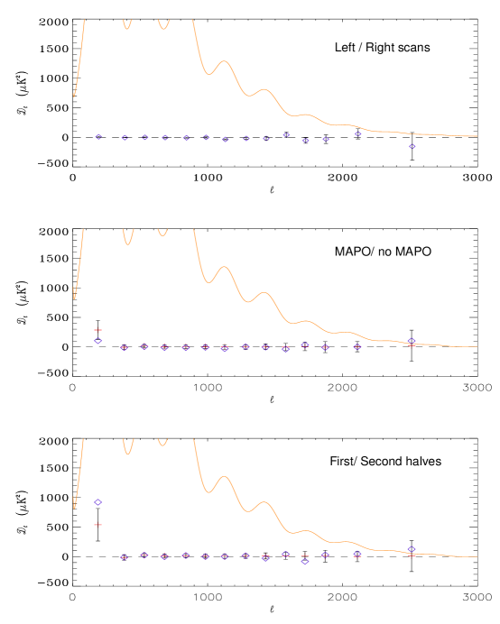
Figure 9: Power spectra of difference maps produced from three different data jackknifes. The top panel shows the power spectrum produced from the difference of maps made with left and right going chopper sweeps. The central panel shows the power spectrum produced from the difference of maps made with values of azimuth toward and away from the MAPO building. The bottom panel shows the power spectrum produced from the difference of maps made from the first and second halves of the data for each of the observed fields CMB2a, CMB2b, CMB5a, and CMB5b. In the central and bottom panels the predicted residuals (cross) and uncertainties are determined by 300 Monte Carlo simulations of each difference map and include effects of incomplete subtraction due to atmospheric mode removal. In all cases, the difference band-powers (diamond) are consistent with there being no significant signal in the subtracted maps. These tests indicate that the noise estimate is accurate and the band-power results are free from significant systematic errors.

Two maps were created by separating the data into two halves corresponding to the left-going and right-going portions of each chopper sweep. The power spectra of the difference between these maps should be sensitive to systematic errors due to chopper induced microphonic response or detector time constants. Because the left and right going sweeps are carried out in exactly the same atmospheric conditions and are subject to the same mode removal, there is no expected residual in the subtracted maps. The power spectrum derived from the L/R differenced data is shown in the top panel of Figure 9. The error bars on the differenced map power spectra are derived from the Fisher matrix. The resulting power spectrum is consistent with there being no systematic difference between the maps.

Next, the data were separated by the azimuth of the observations into two halves corresponding to observations with the telescope pointing in the $180^{\circ}$ azimuth ranges toward and away from the nearby Martin A. Pomerantz Observatory (MAPO) building. The MAPO building is the largest object on the otherwise smooth horizon seen by Acbar at the Pole and is expected to be the largest source of systematic signal due to the modulation of the far sidelobes of the Acbar beams. Therefore, the power spectrum for the differenced map is a sensitive test for ground pickup that is not removed by the LMT differencing. The resulting power spectra is plotted in the middle panel of Figure 9; the results are consistent with the the residual calculated from the Monte Carlo simulation.

In order to test for systematic changes in pointing, calibration or beamsize over the course of the observations, we also create a difference map by separating the data in time. As described in § 3, each of the CMB fields observed actually consists of two subfields offset from one another by $0.5^{\circ}\sec\delta$. Due to changes in beamshape across the chopper swing, there are subtle differences between the subfield maps that could lead to a non-zero residual signal when these maps are subtracted. However, when the maps are added, the resulting beams are represented by the sum of the beams in the input maps and the power spectrum should be unbiased. In order to avoid these complications, differenced maps are created from the first and second halves of the data for each of the four observed subfields CMB2a, CMB2b, CMB5a, and CMB5b. Because the data from which the maps are produced are well separated in time and are subject to different atmospheric mode removal, the predicted residuals for the subtracted maps can be significant on large angular scales. The lower panel of Figure 9 shows the deference map power spectrum with the Monte Carlo determined residuals and uncertainties; again, there is no evidence for significant excess power in the difference map.

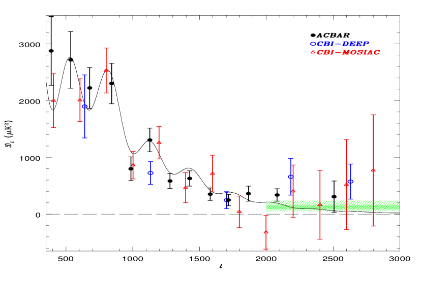
Figure 10: The CMB angular power spectrum for the CBI-Deep, CBI-Mosaic, and Acbar experiments. The data are plotted on top of a fiducial $\Lambda$CDM model. The shaded green bar shows the expected contribution to the ACBAR power spectrum if the excess power found in the CBI-Deep data is due to the SZE. The ACBAR data are consistent with the CBI excess being due to SZE, but provide no signifincant new constraints on the source of the signal.

8 Conclusion

We have used the Acbar receiver to measure the angular power spectrum of the CMB at a frequency of $150\,$GHz over the multipole range $\ell=100-3000$. The power spectrum we present is derived from approximately 21 weeks of Austral winter observations with Acbar installed on the $2.1\,$m Viper telescope at the South Pole.

In the course of analyzing this data, we have employed new analysis techniques designed specifically for high sensitivity ground based CMB observations. Monte Carlo simulations are used to verify that the analysis method accurately recovers the power spectrum without bias. The power spectrum we present is robust and has passed stringent tests for systematic errors. Galactic dust emission and radio point sources do not contribute significantly to the observed power and are projected out in the final analysis. Although dusty protogalaxies cannot be ruled out as a source of confusion, the expected contribution to the measured power is negligible. Overall, the resulting power spectrum appears to be consistent with the damped acoustic oscillations expected in standard cosmological models. In a companion paper (Goldstein et al. 2002), the Acbar power spectrum is used to place constraints on cosmological models. The power in the highest $\ell$ Acbar bin is consistent with the excess power measured in the Deep CBI pointings. At this point, the Acbar data lack the sensitivity to place significant constraints on the origin of the excess power observed by CBI.

We acknowledge assistance in the design and construction of Acbar by the UC Berkeley machine and electronics shop staff. The support of Center for Astrophysics Research in Antarctica (CARA) polar operations has been essential in the installation and operation of the telescope. Percy Gomez, Kathy Romer, and Kim Coble are thanked for their assistance in monitoring the observations and telescope pointing. We thank Nils Halverson, Julian Borrill, and Radek Stompor for a careful reading of the draft and useful comments on analysis algorithms. Finally, we would like to thank John Carlstrom, the director of CARA, for his early and continued support of the project. The ACBAR program has been primarily supported by NSF office of polar programs grants OPP-8920223 and OPP-0091840. This research used resources of the National Energy Research Scientific Computing Center, which is supported by the Office of Science of the U.S. Department of Energy under Contract No. DE-AC03-76SF00098. Chao-Lin Kuo acknowledges support from a Dr. and Mrs. CY Soong fellowship and Marcus Runyan acknowledges support from a NASA Graduate Student Researchers Program fellowship. Chris Cantalupo, Matthew Newcomb and Jeff Peterson acknowledge partial financial support from NASA LTSA grant NAG5-7926.

Appendix A A. Noise Estimate

Each Acbar data file contains observations at $n_{d}$ pointings in declination. Observations at each declination consist of lead, main, and trail pointings in RA which we refer to as stares. Each lead or trail stare has $2n_{s}$ ($n_{s}$ left going and $n_{s}$ right going) chopper sweeps, while the main stares have $4n_{s}$ sweeps. Each sweep contains $n_{x}$ samples of the detector signals. The goal is to estimate the noise correlation in the $M-(L+T)/2$ differenced, coadded maps for each file, and then use this noise correlation in eq. [9] to derive the final pixel space correlation matrix ${\bf C}_{N}$. In order to get better statistics for the noise determination, the noise for each sweep is calculated before the sweeps are coadded so that there are as many realizations as possible.

A file is divided into $n_{d}\times n_{s}$ sets of sweeps, each containing $(2,4,2)$ sweeps in the (L,M,T) fields on $n_{d}$ strips in declination. The sweeps in the sets of stares are grouped by their time order so that the first sets contains the first sweeps from each stare and the last set contains the last sweeps. The sets of sweeps are combined (using $M-(L+T)/2$) to form a $n_{x}$-component data vector for each set of sweeps. The correlations are computed from the LMT subtracted sets of sweeps.

The data for one channel is now reduced to the array data[$n_{x}$,$n_{d}$,$n_{s}$] which we write as $D_{i,j,k}$. Assuming that the data are dominated by noise, the following moments can be determined

$$m_{1}(i,j) =\langle D_{i,\ell,k}\times D_{j,\ell,k}\rangle_{\{\ell,k\}},$$

$$m_{2}(i,j,\Delta s) =\langle D_{i,\ell,k}\times D_{j,\ell,k+\Delta s}\rangle_{\{\ell,k\}},$$

$$m_{3}(i,j,\Delta d,\Delta s) =\langle D_{i,\ell,k}\times D_{j,\ell+\Delta d,k+\Delta s}\rangle_{\{\ell,k\}}.$$

They are interpreted as correlations within a data strip ($m_{1}$), among data strips in a constant declination ($m_{2}$), and among different declinations ($m_{3}$). These are all correlations within the same channel. There are also cross-channel correlations for $m_{1},$ etc., that are also largely due to the atmosphere.

As was pointed out in §4, the pixel space correlation matrix is simply the weighted average of ${\bf\Pi}{\bf N}{\bf\Pi}^{t}$, or $\langle\tilde{\bf d}\tilde{\bf d}^{t}\rangle$. One could calculate it directly from “cleaned” timestream $\tilde{\bf d}$, however after the mode removal, the correlation within a sweep is not just a function of $|i-j|$ anymore, instead it is a function of both $i$ and $j$. This prevents the application of Wiener-Khinchin theorem (PSD $\leftarrow{FFT}\rightarrow$ ACF) and would make the algorithm time consuming. Instead, the correlation is determined before the projection destroys the “stationary” property of the noise by calculating ${\bf N}=\langle{\bf dd}^{t}\rangle$ first, then using $\langle\tilde{\bf d}\tilde{\bf d}^{t}\rangle={\bf\Pi}\langle{\bf dd}^{t}\rangle{\bf\Pi}^{t}$. In Appendix B, the application of the FFT for piecewise stationary random processes such as the Acbar noise is described. A PSD is by definition positive. Due to limited numbers of realizations the PSD calculated from the ACF is not always positive. We therefore parametrize the PSD with the first three terms of the Laurent series,

$$PSD=a_{0}+a_{1}f^{-1}+a_{2}f^{-2}\,,$$

with the constraint that $a_{i}>0$. This expression is found to be an excellent description of the noise PSD.

In principle, the chopper synchronous offset could introduce correlations between declinations. In practice, these correlations are effectively removed by the $M-(L+T)/2$ differencing. In the vast majority of the data, $m_{3}$ is consistent with zero. It is also found that when the atmosphere is calm, $m_{2}$ is also small ($<5\%$) after LMT subtraction and projection of corrupted modes. These cross-sweep correlations are included in the noise correlation matrix, but are not found to not have a significant effect on the noise estimate. Nonetheless, approximately $\sim 20-30\%$ of the data was cut because it showed a significant residual correlation ($m_{2}>5\%$) between sweeps after atmospheric removal.

Although the data used in the analysis are dominated by the instrument noise, atmospheric induced cross-channel correlations must be taken into account. Although they are small, the inclusion of the cross channel correlations can lead to a noise correlation matrix that is not guaranteed to be positive definite. Including these correlations (and removing the negative eigenmodes in the S/N transformation [D]) does not appear to effect the resulting power spectrum, however, it does introduce an element of uncertainty to the analysis. To avoid this complication, the band-powers presented in this paper are calculated without including cross-channel correlations. This results in a small uncertainty in the noise estimate equal to the largest measured fractional cross-channel correlation. By cutting an additional $10\%$ of the data observed to have a correlation exceeding 5%, we can guarantee that the noise estimate is correct to this level. From the distribution of channel correlations, we estimate the real error in the noise estimate to be much smaller. The power spectrum presented in this paper is insensitive to uncertainty in the noise estimate at the level of a few percent.

Appendix B B. Correlation and FFT

The calculation of the various moments described in Appendix A can be done by Fast Fourier transformation. One slight complication is Fourier transformation assumes the input data to be periodic. For a strictly stationary process this is not a problem since the correlation usually vanishes after a sufficiently long time lag. For piecewise stationary processes, a straightforward application of FFT produces false correlation for lag $>n/2$ , where $n$ is the number of elements. This can be prevented by zero padding.

Suppose we want to calculate the correlation of two real, $n$-component stochastic data vectors ${\bf x}$ and ${\bf y}$. When ${\bf x}$ and ${\bf y}$ are stationary, averaging over indices is ensemble average,

$$C_{ij}\equiv\langle x_{i}y_{j}\rangle=C(\Delta\equiv|i-j|)=\frac{1}{2(n-\Delta)}\sum_{j=1}^{n-\Delta}(x_{j}y_{j+\Delta}+x_{j+\Delta}y_{j}).$$ (B1)

A faster algorithm involves FFT. To prevent periodicity we pad the two data vectors with zeros up to $2n$, and Fourier transform:

$$f_{u}^{*} =\frac{1}{2n}\sum_{j=1}^{2n}x_{j}\exp{\left(\frac{i\pi uj}{n}\right)},$$

$$g_{u} =\frac{1}{2n}\sum_{k=1}^{2n}y_{k}\exp{\left(-\frac{i\pi uk}{n}\right)}.$$

The inverse Fourier transform of $f^{*}g$ is

$$FFT^{-1}({\bf f^{*}g}) \equiv\frac{1}{(2n)^{2}}\sum_{jku=1}^{2n}x_{j}y_{k}\exp{\left[-\frac{i\pi u}{n}(k-j)\right]}\cdot\exp{\left(\frac{i\pi u\Delta}{n}\right)}$$

$$=\frac{1}{(2n)^{2}}\sum_{jk=1}^{2n}x_{j}y_{k}\sum_{u=1}^{2n}\exp{\left[\frac{i\pi u}{n}(j+\Delta-k)\right]}$$

$$=\frac{1}{2n}\sum_{jk=1}^{2n}x_{j}y_{k}(\delta_{j+\Delta,k}+\delta_{j+\Delta,k\pm 2n}+\delta_{j+\Delta,k\pm 4n}+\cdots)$$

$$=\frac{1}{2n}\sum_{jk=1}^{2n}x_{j}y_{k}(\delta_{j+\Delta,k})=\frac{1}{2n}\sum_{j=1}^{2n}x_{j}y_{j+\Delta}=\frac{1}{2n}\sum_{j=1}^{n-\Delta}x_{j}y_{j+\Delta}.$$

The last step uses the fact that $y_{k}=0$ for $k>n$. Comparing this with eq. [B1], we obtain

$$C(\Delta)=\frac{n}{n-\Delta}FFT^{-1}({\bf f^{*}g}+{\bf fg^{*}})=\frac{2n}{n-\Delta}FFT^{-1}[\,{\Re}({\bf f^{*}g})\,].$$ (B2)

Note that with the correction factor $2n/(n-\Delta)$, eq. [B2] is exact for $0\leq\Delta\leq n-1$. $C(\Delta)$ were then averaged for 20 minutes to improve signal-to-noise.

In the presence of a data cut, for example the guiding quasar, a similar “pad-and-correct” procedure can be used, such that the data corrupted by the quasar will be ignored in the calculation of correlation function.

Appendix C C. Theory Matrix for Non-uniform Beams

For a given 2-D power spectrum density $P({\bf k})$, the Fourier transform of the temperature map $T({\hat{\bf r}})$, or the spectrum is

$$S({\bf k})=\sqrt{\frac{P({\bf k})}{2}}{\cal B}({\bf k})\zeta({\bf k}),$$

where $\cal B$ is the Fourier transform of the response function at ${\hat{\bf r}}=(x,y)$, and $\zeta$ a Gaussian random variable: $\zeta({\bf k})=\zeta_{r}({\bf k})+i\zeta_{i}({\bf k})$, $\langle\zeta_{r}^{2}\rangle=\langle\zeta_{i}^{2}\rangle=1$. The realization condition requires that

$$P({\bf k})=P(-{\bf k});\;\;\;\;\zeta^{*}({\bf k})=\zeta(-{\bf k}).$$

Note that $\langle\zeta^{*}({\bf k})\zeta({\bf k^{\prime}})\rangle=2\delta({\bf k}-{\bf k^{\prime}})$, which is a natural consequence of Gaussian random variables. The realization condition does not introduce new correlation because $\langle\zeta^{*}({\bf k})\zeta(-{\bf k})\rangle=\langle\zeta^{*}({\bf k})\zeta^{*}({\bf k})\rangle=\langle\zeta_{r}^{2}({\bf k})\rangle-\langle\zeta_{i}^{2}({\bf k})\rangle=0$.

The temperature correlation is

$$C_{T\{12\}}=\langle T^{*}({\hat{\bf r}}_{1})T({\hat{\bf r}}_{2})\rangle=\iint d{\bf k}d{\bf k^{\prime}}\exp\left\{-2\pi i[-{\bf k\cdot}{\hat{\bf r}}_{1}+{\bf k^{\prime}}{\bf\cdot}{\hat{\bf r}}_{2}]\right\}\langle S^{*}_{1}({\bf k})S_{2}({\bf k^{\prime}})\rangle$$

$$=\iint d{\bf k}d{\bf k^{\prime}}\exp\left\{-2\pi i[-{\bf k\cdot}{{\hat{\bf r}}}_{1}+{\bf k^{\prime}}{\bf\cdot}{\hat{\bf r}}_{2}]\right\}{\cal B}^{*}_{1}({\bf k}){\cal B}_{2}({\bf k^{\prime}})\times\frac{\sqrt{P({\bf k})P({\bf k^{\prime}})}}{2}\langle\zeta^{*}({\bf k})\zeta({\bf k^{\prime}})\rangle$$

$$=FFT^{-1}\left[P({\bf k}){\cal B}^{*}_{1}({\bf k}){\cal B}_{2}({\bf k})\right]_{({\hat{\bf r}}={\hat{\bf r}}_{2}-{\hat{\bf r}}_{1})}.$$

What we really want to know for band-power estimation is the derivative of $C_{T\{12\}}$ with respect to the band-power $q_{B}$. This is easily done by replacing $P$ in the equation above with proper shape functions determined by $\chi_{B\ell}$ defined in eq. [12]. For simplicity we made $\chi_{B\ell}$ flat in $D_{\ell}$. In terms of P the filter functions acquire corrections from the transformation between $D_{\ell}$ and $C_{\ell}$ , hence are not flat in band. We parameterize a Gaussian beam as

$$B_{0}(x,y)\propto\exp(-\frac{u}{2});\;\;\;\;u\equiv\frac{1}{2}\left[(\frac{x}{\alpha}+\frac{y}{\beta})/\gamma\right]^{2}+\frac{1}{2}\left(\frac{x}{\alpha}-\frac{y}{\beta}\right)^{2}.$$

In this parametrization, if $(\alpha,\beta,\gamma)=(\sigma,\sigma,1)$, $B_{0}$ is an axisymmetric Gaussian function with FWHM $\sigma\sqrt{8\ln 2}$. In the wavenumber domain, the total experimental response function is

$${\cal B}({\bf k})={\tilde{\Xi}}({\bf k})\times\exp\left\{-\frac{4\pi^{2}}{2}\left[\frac{\gamma^{2}(k_{x}\alpha+k_{y}\beta)^{2}}{2}+\frac{(k_{x}\alpha-k_{y}\beta)^{2}}{2}\right]\right\}.$$

Here ${\tilde{\Xi}}({\bf k})$ is the Fourier transform of LMT switching pattern $\Xi({\hat{\bf r}})$ defined in eq.[10]. For a pair of pixels (1,2),

$${\cal B}^{*}_{1}({\bf k}){\cal B}_{2}({\bf k})=|{\tilde{\Xi}}({\bf k})|^{2}\exp\left\{-4\pi^{2}\left[(\mu_{1}+1)\sigma_{x}^{2}k_{x}^{2}+(\mu_{2}+1)\sigma_{y}^{2}k_{y}^{2}+\mu_{3}\sigma_{x}\sigma_{y}k_{x}k_{y}\right]\right\},$$

where

$$\mu_{1}\equiv\frac{[(\gamma_{1}^{2}+1)\alpha_{1}^{2}+(\gamma_{2}^{2}+1)\alpha_{2}^{2}]}{4\sigma_{x}^{2}}-1,$$

$$\mu_{2}\equiv\frac{[(\gamma_{1}^{2}+1)\beta_{1}^{2}+(\gamma_{2}^{2}+1)\beta_{2}^{2}]}{4\sigma_{y}^{2}}-1,$$

$$\mu_{3}\equiv\frac{[(\gamma_{1}^{2}-1)\alpha_{1}\beta_{1}+(\gamma_{2}^{2}-1)\alpha_{2}\beta_{2}]}{2\sigma_{x}\sigma_{y}}.$$

Here $(\sigma_{x},\sigma_{y})$ are taken to be the average of beam RMS in RA and DEC. To the zeroth order in ${\boldsymbol{\mu}}$,

$$C_{T\{12\}}({\boldsymbol{\mu}})\sim C_{T\{12\}}(0)=FFT^{-1}\left\{P({\bf k})|{\tilde{\Xi}}({\bf k})|^{2}\exp\left[-4\pi^{2}(\sigma_{x}^{2}k_{x}^{2}+\sigma_{y}^{2}k_{y}^{2})\right]\right\}_{({\hat{\bf r}}={\hat{\bf r}}_{2}-{\hat{\bf r}}_{1})}.$$

Since $\ell=4\pi\sqrt{k_{x}^{2}+k_{y}^{2}}$, if $\sigma_{x}=\sigma_{y}$, ${\cal B}^{2}$ reduces to the well known beam smearing function $B_{\ell}=\exp{(-\sigma^{2}\ell^{2})}$ for a symmetric Gaussian beam.

We can obtain next order approximation of $C_{T\{12\}}$ by taking its partial derivatives in ${{\boldsymbol{\mu}}}$:

$$\frac{\partial C_{T\{12\}}}{\partial\mu_{1}}{\Bigg{|}}_{{{\boldsymbol{\mu}}}=0} =FFT^{-1}\left\{(-4\pi^{2}\sigma_{x}^{2}k_{x}^{2})P({\bf k})|{\tilde{\Xi}}({\bf k})|^{2}\exp\left[-4\pi^{2}(\sigma_{x}^{2}k_{x}^{2}+\sigma_{y}^{2}k_{y}^{2})\right]\right\}_{({\hat{\bf r}}={\hat{\bf r}}_{2}-{\hat{\bf r}}_{1})};$$

$$\frac{\partial C_{T\{12\}}}{\partial\mu_{2}}{\Bigg{|}}_{{{\boldsymbol{\mu}}}=0} =FFT^{-1}\left\{(-4\pi^{2}\sigma_{y}^{2}k_{y}^{2})P({\bf k})|{\tilde{\Xi}}({\bf k})|^{2}\exp\left[-4\pi^{2}(\sigma_{x}^{2}k_{x}^{2}+\sigma_{y}^{2}k_{y}^{2})\right]\right\}_{({\hat{\bf r}}={\hat{\bf r}}_{2}-{\hat{\bf r}}_{1})};$$

$$\frac{\partial C_{T\{12\}}}{\partial\mu_{3}}{\Bigg{|}}_{{{\boldsymbol{\mu}}}=0} =FFT^{-1}\left\{(-4\pi^{2}\sigma_{x}\sigma_{y}k_{x}k_{y})P({\bf k})|{\tilde{\Xi}}({\bf k})|^{2}\exp\left[-4\pi^{2}(\sigma_{x}^{2}k_{x}^{2}+\sigma_{y}^{2}k_{y}^{2})\right]\right\}_{({\hat{\bf r}}={\hat{\bf r}}_{2}-{\hat{\bf r}}_{1})};$$

$$\;\;\;\vdots$$

$${\rm etc.}$$

The first few terms of $C_{T\{12\}}$ are

$$C_{T\{12\}}({\boldsymbol{\mu}})=C_{T\{12\}}({\boldsymbol{\mu}}=0)+\sum_{i}\left(\frac{\partial C_{T\{12\}}}{\partial\mu_{i}}{\Bigg{|}}_{{{\boldsymbol{\mu}}}=0}\right)\mu_{i}$$

$$+\frac{1}{2!}\sum_{ij}\left(\frac{\partial^{2}C_{T\{12\}}}{\partial\mu_{i}\partial\mu_{j}}{\Bigg{|}}_{{{\boldsymbol{\mu}}}=0}\right)\mu_{i}\mu_{j}+\cdots$$

The largest corrections occur at high $\ell$. For $\ell\sim 2000$, FWHM $\sim 5.5^{\prime}$ and a $10\%$ beam distortion ($\mu=0.1$), the leading order correction is on the order of $4\pi^{2}\sigma^{2}k^{2}\mu\sim 20\%$ for that specific pixel pair. However, since $(\sigma_{x},\sigma_{y})$ are the noise weighted average beam sizes, the correction goes both ways and the resulting power spectrum does not change significantly.

Appendix D D. Signal-to-Noise Eigenmode Truncation and Foreground Removal

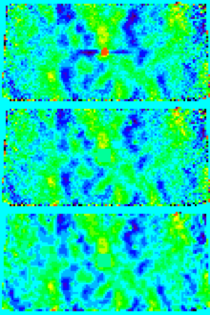
Figure 11: The three panels show the noise weighted coadded map ${\bf T}$ (top), the foreground removed map ${{\bf T}}^{\prime}_{r}$ (middle), and the high signal-to-noise map ${{\bf T}}^{\prime}_{s}$ (bottom). The top panel is the noise weighted coadded map for the CMB5 field; it shows the bright quasar and the artifact generated from mode removal (the blue horizontal stripes adjacent to the quasar). The second panel shows the same map after the foreground modes defined in Table 4 are set to zero and ignored in the power spectrum calculation. Other than the bright guiding quasar, there are no other clear sources of significant foreground emission. This qualitative statement is supported by the fact that after the removal of the guide quasar, the power spectrum derived from this field is unchanged by the removal of the radio source and galactic dust templates. The bottom panel shows foreground removed map constructed from only the high S/N eigenmodes. Clearly, the S/N eigenmode transformation preserves the basic features of the map.

The constraint matrix formalism is typically used to remove undesired foreground modes (Bond et al. 1998; Halverson et al. 2002; Meyers et al. 2002). Combined with signal-to-noise eigenmode analysis (Karhunen-Lo’ eve transformation) (Bunn & White 1997; Bond et al. 1998), the foreground removal can be implemented in an alternative algorithm. First we construct the foreground mode projection matrices that remove the modes described in Tables 3 and 4. Similar to §4.1.3, if ${\bf U}$ consists of $m$ columns of linearly independent foreground modes, in our pixel space ${\bf U}$ manifests itself as ${\tilde{\bf U}}={\bf KU}$ (eq. [7]). Following Tegmark (1997), we define the projection matrix ${\bf P}\equiv{\bf I}-{\tilde{\bf U}}({\tilde{\bf U}}^{t}{\tilde{\bf U}})^{-1}{\tilde{\bf U}}^{t}$.

Next we solve for the eigenvalues $\omega_{i}$ and eigenvectors ${\bf e}_{i}$ for the foreground removed noise correlation ${{\bf C}^{\prime}}_{N}\equiv{\bf P}{{\bf C}}_{N}{\bf P}$. The projection of ${\bf P}$ creates a $m$ - dimensional degenerate vector space with eigenvalue zero. Numerically, the eigenvalues of the undesired modes are at least 10 orders of magnitude smaller than that of the desired modes. Assume $\omega_{1}=\omega_{2}=\dots=\omega_{m}=0$. The “whitening” matrix is defined as

$${\bf W}\equiv\begin{bmatrix}\;\;\;\;\arrowvert&\;\;\;\;\arrowvert&\;&\;\;\;\;\;\;\;\arrowvert\\ \omega_{m+1}^{-1/2}{\bf e}_{m+1}&\omega_{m+2}^{-1/2}{\bf e}_{m+2}&\dots&\omega_{n}^{-1/2}{\bf e}_{n}\\ \;\;\;\;\downarrow&\;\;\;\;\downarrow&\;&\;\;\;\;\;\;\;\downarrow\end{bmatrix},$$

such that ${\bf W}^{t}{{\bf C}}^{\prime}_{N}{\bf W}={\bf I}$, where ${\bf I}$ is the $n-m\equiv m_{1}$ dimensional identity matrix. After the transformation of the temperature map by the application of ${\bf W}$, the foreground modes are “projected out” completely, since eigenvectors (${\bf e}_{1},{\bf e}_{2},\cdots{\bf e}_{m}$) with zero eigenvalues are not included in the construction of ${\bf W}$. To proceed with the signal-to-noise eigenmode transformation, we construct a fiducial theory matrix that is compared with the noise matrix to decide which modes contain useful information (high S/N). The theory matrix ${{\bf C}}_{T}=\sum_{B}q_{B}{\partial{{\bf C}}_{T}}/{\partial q_{B}}$, where the $q_{B}$’s are the band powers we wish to estimate. The most reasonable choice of a fiducial power spectrum is a constant flat band-power $\Sigma^{2}=10^{4}\,\mu{\rm K}^{2}$, chosen as a conservative upper bound for $D_{\ell}$. The application of W to the fiducial theory matrix and temperature map removes the corrupted foreground modes: ${{\bf C}}_{T}\rightarrow{\bf W}^{t}{{\bf C}}_{T}{\bf W};$ $\;\;\;{{\bf T}}\rightarrow{\bf T}_{r}\equiv{\bf W}^{t}{{\bf T}}$.

By operating on ${\bf W}^{t}{{\bf C}}_{T}{\bf W}$ with its orthonormal matrix ${\bf R}$, it can be diagonalized;

$${\bf W}^{t}{{\bf C}}_{T}{\bf W}\rightarrow{\bf R}^{t}{\bf W}^{t}{{\bf C}}_{T}{\bf W}{\bf R}\equiv{\boldsymbol{\mathcal{E}}}={\rm diag}({\cal E}_{k}).$$

In this new basis, the theory matrix consists of diagonal elements of signal-to-noise values ${\cal E}_{k}$. Modes corresponding to small ${\cal E}_{k}$ do not significantly contribute to the likelihood function and only the $n_{s}$ high S/N modes are retained. For the CMB2 field the number of modes was decreased from 9000 to 2500, and for CMB5 the reduction was from 5000 to 2000. Eliminating these “noisy” modes greatly reduced the computational resources required by the quadratic iteration described in §4.4.2. The first $n_{s}$ columns of ${\bf R}$ form a $m_{1}\times n_{s}$ transformation matrix ${\bf R}_{1}$. The foreground subtracted, high S/N mode data are ${\bf T}_{s}\equiv{\bf R}_{1}^{t}{\bf W}^{t}{{\bf T}}$; and the noise correlation matrix is the $n_{s}$ dimensional identity matrix. The resulting CMB power spectrum is unchanged for values of the cut-off S/N ranging from ${\cal E}_{c}=0.1$ to $0.01$; this is a direct consequence of the conservative choice of $\Sigma^{2}$. The results presented in this paper were calculated using ${\cal E}_{c}=0.05$.

To demonstrate the foreground removal and Karhunen-Lo’ eve transformation in effect, it is useful to reconstruct the pixel-space map from the lower dimensional ${\bf T}_{r}$ and ${\bf T}_{s}$ data vectors,

$${{\bf T}}^{\prime}_{r} ={\bf W}{\bf\Theta}{\bf T}_{r};$$

$${{\bf T}}^{\prime}_{s} ={\bf W}{\bf\Theta}{\bf R}_{1}{\bf T}_{s},$$

where ${\bf\Theta}={\rm diag}(\omega_{k}),\;\;\;(k=m+1,\;,m+2,\dots,n)$. ${{\bf T}^{\prime}}_{r}$ is the foreground-removed map, and ${{\bf T}^{\prime}}_{s}$ is the foreground-removed map reconstructed only from high signal-to-noise modes. ${{\bf T}^{\prime}}_{r}$ and ${{\bf T}^{\prime}}_{s}$ are both $n$ dimensional, can be directly compared with the raw coadded map ${{\bf T}}$. The foreground removed maps for the CMB2 and CMB5 fields are shown in Figures 5 and 6. For comparison, the raw coadded map, the foreground-free map, and the high S/N eigenmode maps for the CMB5 field are shown in Figure 11.

References

- Abroe et al. (2002) Abroe, M. E., Balbi, A., Borrill, J., Bunn, E. F., Hanany, S., Ferreira, P. G., Jaffe, A. H., Lee, A. T., Olive, K. A., Rabii, B., Richards, P. L., Smoot, G. F., Stompor, R., Winant, C. D., & Wu, J. H. P. 2002, MNRAS, 334, 11
- Blain et al. (1998) Blain, A. W., Ivison, R. J., & Smail, I. 1998, MNRAS, 296, L29
- Bond et al. (2002) Bond, J. R., Contaldi, C. R., Pen, U.-L., Pogosyan, D., Prunet, S., Ruetalo, M. I., Wadsley, J. W., Zhang, P.and Mason, B. S., Myers, S. T., Pearson, T. J., Readhead, A. C. S., Sievers, J. L., & Udomprasert, P. S. 2002, Submitted to ApJ, astro-ph/0205386
- Bond & Efstathiou (1987) Bond, J. R. & Efstathiou, G. 1987, MNRAS, 226, 655
- Bond et al. (1998) Bond, J. R., Jaffe, A. H., & Knox, L. 1998, Phys. Rev. D, 57, 2117
- Bond et al. (2000) —. 2000, ApJ, 533, 19, astro-ph/9808264
- Bunn & White (1997) Bunn, E. F. & White, M. 1997, ApJ, 480, 6
- Chamberlin (2001) Chamberlin, R. A. 2001, J. Geophys. Res., 106, 20101
- Cooray & Melchiorri (2002) Cooray, A. & Melchiorri, A. 2002, Phys. Rev. D, in press, astro-ph/0204250
- Dawson et al. (2002) Dawson, K. S., Holzapfel, W. L., Carlstrom, J. E., Joy, M., LaRoque, S. J., & Reese, E. D. 2002, ApJ, in press, astro-ph/020601
- Ferreira & Jaffe (2000) Ferreira, P. G. & Jaffe, A. H. 2000, MNRAS, 312, 89
- Finkbeiner et al. (1999) Finkbeiner, D. P., Davis, M., & Schlegel, D. J. 1999, ApJ, 524, 867
- Goldstein et al. (2002) Goldstein, J., Ade, A. R., Bock, J. J., Bond, J. R., Cantaldi, C., Daub, M. D., Holzapfel, W. L., Kuo, C. L., Lange, A. E., Newcomb, M., Peterson, J. B., Pogosyan, D., Ruhl, J., Runyan, M. C., & Torbet, E. 2002, In Preperation
- Gomez et al. (2002) Gomez, P., Romer, K., Cantalupo, C., Peterson, J., Goldstein, J., Daub, M. D., Holzapfel, W. L., Kuo, C. L., Lange, A. E., Newcomb, M., Ruhl, J., Runyan, M. C., & Torbet, E. 2002, In Preparation
- Griffin et al. (1986) Griffin, M. J., Ade, P. A. R., Orton, G. S., Robson, E. I., Gear, W. K., Nolt, I. G., & Radostitz, J. V. 1986, Icarus, 65, 244
- Griffin & Orton (1993) Griffin, M. J. & Orton, G. S. 1993, Icarus, 105, 537
- Griffiths et al. (2002) Griffiths, L. M., Kunz, M., & Silk, J. 2002, Preprint, astro-ph/0204100
- Halverson (2002) Halverson, N. W. 2002, PhD thesis, Caltech
- Halverson et al. (2002) Halverson, N. W., Leitch, E. M., Pryke, C., Kovac, J., Carlstrom, J. E., Holzapfel, W. L., Dragovan, M., Cartwright, J. K., Mason, B. S., Padin, S., Pearson, T. J., Readhead, A. C. S., & Shepherd, M. C. 2002, ApJ, 568, 38
- Holder et al. (2001) Holder, G., Haiman, Z., & Mohr, J. J. 2001, ApJ, 560, L111
- Hu et al. (1997) Hu, W., Sugiyama, N., & Silk, J. 1997, Nature, 386, 37, astro-ph/9604166
- Hu & White (1996) Hu, W. & White, M. 1996, ApJ, 471, 30
- Hu & White (1997) —. 1997, ApJ, 479, 568
- Jaffe et al. (2001) Jaffe, A. H., Ade, P. A. R., Balbi, A., Bock, J. J., Bond, J. R., Borril, J., Boscaleri, A., Coble, K., & Crill, B. P. 2001, Phys. Rev. Lett., 86, 3475, astro-ph/0007333
- Knox (1999) Knox, L. 1999, Phys. Rev. D, 60, 103516, astro-ph/9902046
- Komatsu & Seljak (2002) Komatsu, E. & Seljak, U. 2002, MNRAS, 336, 1256
- Lange et al. (2001) Lange, A. E., Ade, P. A. R., Bock, J. J., Bond, J. R., Borrill, J., Boscaleri, A., Coble, K., Crill, B. P., de Bernardis, P., Farese, P., Ferreira, P., Ganga, K., Giacometti, M., Hivon, E., Hristov, V. V., Iacoangeli, A., Jaffe, A. H., Martinis, L., Masi, S., Mauskopf, P. D., Melchiorri, A., Montroy, T., Netterfield, C. B., Pascale, E., Piacentini, F., Pogosyan, D., Prunet, S., Rao, S., Romeo, G., Ruhl, J. E., Scaramuzzi, F., & Sforna, D. 2001, Phys. Rev. D., 63, 042001
- Lay & Halverson (2000) Lay, O. P. & Halverson, N. W. 2000, ApJ, 543, 787
- Lee et al. (2001) Lee, A. T., Ade, P., Balbi, A., Bock, J., Borrill, J., Boscaleri, A., de Bernardis, P., Ferreira, P. G., Hanany, S., Hristov, V. V., Jaffe, A. H., Mauskopf, P. D., Netterfield, C. B., Pascale, E., Rabii, B., Richards, P. L., Smoot, G. F., Stompor, R., Winant, C. D., & Wu, J. H. P. 2001, ApJ, 561, L1
- Mason et al. (2002) Mason, B. S., Pearson, T., Readhead, A. C. S., Shephard, M. C., Sievers, J. L., Udomprasert, P. S., Cartwright, J. K., Farmer, A. J., Padin, S., Myers, S. T., Bond, J. R., Contaldi, C. R., Pen, U.-L., Prunet, S., Pogosyan, D., Carlstom, J. E., Kovac, J., Leitch, E., Pryke, C., Halverson, N., Holzapfel, W., Altamirano, P., Brofman, L., Casassus, S., May, J., & Joy, M. 2002, Submitted to ApJ, astro-ph/0205384
- Meyers et al. (2002) Meyers, S. T., Contaldi, C. R., Bond, J. R., Pen, U.-L., Pogosyan, D., Prunet, S., Sievers, J. L., Mason, B. S., Pearson, T., Readhead, A. C. S., & Shephard, M. C. 2002, ApJ, submitted, astro-ph/0205385
- Miller et al. (1999) Miller, A. D., Caldwell, R., Devlin, M. J., Dorwart, W. B., Herbig, T., Nolta, M. R., Page, L. A., Puchalla, J., Torbet, E., & Tran, H. T. 1999, ApJ, 524, L1
- Netterfield et al. (2002) Netterfield, C. B., Ade, P. A. R., Bock, J. J., Bond, J. R., Borrill, J., Boscaleri, A., Coble, K., Contaldi, C. R., Crill, B. P., de Bernardis, P., Farese, P., Ganga, K., Giacometti, M., Hivon, E., Hristov, V. V., Iacoangeli, A., Jaffe, A. H., Jones, W. C., Lange, A. E., Martinis, L., Masi, S., Mason, P., Mauskopf, P. D., Melchiorri, A., Montroy, T., Pascale, E., Piacentini, F., Pogosyan, D., Pongetti, F., Prunet, S., Romeo, G., Ruhl, J. E., & Scaramuzzi, F. 2002, ApJ, 571, 604
- Netterfield et al. (1997) Netterfield, C. B., Devlin, M. J., Jarolik, N., Page, L., & Wollack, E. J. 1997, ApJ, 474, 47
- Peterson et al. (2000) Peterson, J. B., Griffin, G. S., Newcomb, M. G., Alvarez, D. L., Cantalupo, C. M., Morgan, D., Miller, K. W., Ganga, K., Pernic, D., & Thoma, M. 2000, ApJ, 532, L83
- Peterson et al. (2002) Peterson, J. B., Radford, S. J. E., Ade, P. A. R., Chamberlin, R. A., O’Kelly, M. J., Peterson, K. M., & Schartman, E. 2002, submitted to ApJ, astro-ph/0205350
- Pryke et al. (2002) Pryke, C., Halverson, N. W., Leitch, E. M., Kovac, J., Carlstrom, J. E., Holzapfel, W. L., & Dragovan, M. 2002, ApJ, 568, 46
- Runyan et al. (2002a) Runyan, M. C., Daub, M. D., Goldstein, J., Holzapfel, W. L., Kuo, C. L., Lange, A. E., Newcomb, M., Peterson, J. B., Ruhl, J., & Torbet, E. 2002a, In Preparation
- Runyan et al. (2002b) —. 2002b, In Preparation
- Saez et al. (1996) Saez, D., Holtmann, E., & Smoot, G. F. 1996, ApJ, 473, 1
- Schlegel et al. (1998) Schlegel, D. J., Finkbeiner, D. P., & Davis, M. 1998, ApJ, 500, 525
- Sievers et al. (2002) Sievers, J. L., Bond, J. R., Cartwright, J. K., Contaldi, C. R., Mason, B. S., Myers, S. T., Padin, S., Pearson, T. J., Pen, U.-L., Pogosyan, D., Prunet, S., Readhead, A. C. S., Shepherd, M. C., Udomprasert, P. S., Bronfman, L., Holzapfel, W. L., , & May, J. 2002, Submitted to ApJ, astro-ph/0205387
- Silk (1968) Silk, J. 1968, ApJ, 151, 459
- Sunyaev & Zel’dovich (1970) Sunyaev, R. A. & Zel’dovich, Y. B. 1970, Ap&SS, 7, 3
- Tegmark (1997) Tegmark, M. 1997, Phys. Rev. D, 55, 5895
- Tegmark & et al. (1999) Tegmark, M. & et al. 1999, in ASP Conf. Ser. 181: Microwave Foregrounds, 3–+
- Ulich (1981) Ulich, B. L. 1981, AJ, 86, 1619
- Weisstein (1996) Weisstein, E. W. 1996, Ph.D. Thesis
- White (2001) White, M. 2001, ApJ, 555, 88
- White et al. (2002) White, M., Hernquist, L., & Springel, V. 2002, ApJ, 579, 16
- White et al. (1994) White, M., Scott, D., & Silk, J. 1994, ARA&A, 32, 319
- Wright et al. (1994) Wright, A. E., Griffith, M. R., Burke, B. F., & Ekers, R. D. 1994, ApJS, 91, 111
- Wu et al. (2001) Wu, J. H. P., Balbi, A., Borrill, J., Ferreira, P. G., Hanany, S., Jaffe, A. H., Lee, A. T., Oh, S., Rabii, B., Richards, P. L., Smoot, G. F., Stompor, R., & Winant, C. D. 2001, ApJS, 132, 1
- Zhang et al. (2002) Zhang, P., Pen, U., & Wang, B. 2002, ApJ, 577, 555