CDM Substructure in Gravitational Lenses: Tests and Results

Abstract

We use a simple statistical test to show that the anomalous flux ratios observed in gravitational lenses are created by gravitational perturbations from substructure rather than propagation effects in the interstellar medium or incomplete models for the gravitational potential of the lens galaxy. We review current estimates that the substructure represents $0.006<f_{sat}<0.07$ (90% confidence) of the lens galaxy mass, and outline future observational programs which can improve the results.

1 Introduction

It is a generic feature of CDM (cold dark matter) halo simulations that a significant fraction of the halo mass remains in the form of satellites (e.g. Kauffmann et al. 1993, Moore et al. 1999, Klypin et al. 1999). The exact mass fraction remains somewhat unclear, but the global mass fraction is of order 5–10%, and the projected fraction inside cylinders of radius $R\sim 5h^{-1}$kpc is of order 1%. These mass fractions are significantly higher than are observed in satellites of the Galaxy, suggesting a conflict between CDM models and observations. Three general classes of solutions have been proposed. First, the satellites can be made invisible by suppressing star formation (Kauffmann et al. 1993; Bullock et al. 2000). Second, they can be destroyed by normal dynamical processes or abnormal ones such as self-interacting dark matter (Spergel & Steinhardt 2000; Yoshida et al. 2000; Colín et al. 2002; D’Onghia & Burkert 2002). Third, their formation might be avoided by significantly reducing the amplitude of the power spectrum on the relevant scales (Kamionkowski & Liddle 2000; Colín et al. 2000; Bode et al. 2001; Avila-Reese et al. 2001). The problem, of course, is that it is difficult to distinguish between undetectable and absent satellites.

It was realized early in the debate (see Moore et al. 1999) that gravitational lensing provided a means of resolving the issue because it could detect the gravitational perturbations created by substructure. It was already known that satellites provided a means of solving the “anomalous flux ratio” problem seen in some gravitational lenses (Mao & Schneider 1998). An example of such a problem is shown in Fig. 1, where the close image pair would be expected to have very similar fluxes for any lens model where the gravitational potential can be well-represented by a low-order Taylor series expansion near the images. Metcalf & Madau (2001) and Chiba (2002) pointed out that such anomalies should be common given the predicted CDM substructure fractions. Mao & Schneider (1998), Keeton (2001), Bradac et al. (2002), and Chiba (2002) explored how substructure could explain the anomalous flux ratios in several lens systems. Metcalf & Zhao (2001), Keeton, Gaudi & Petters (2002) and Evans & Witt (2002) explored whether the model for the primary lens galaxy could be modified to explain the anomalous flux ratios, with mixed results which we will discuss in detail below. Our contribution in Dalal & Kochanek (2002, DK02 hereafter) was to analyze the data to make an experimental determination of the substructure fraction, finding it to be in the range $0.006<f_{sat}<0.07$ (90% confidence) based on a sample of radio lenses. This is in good agreement with the expectations for CDM, and well above standard estimates for the mass fractions in normal satellites.

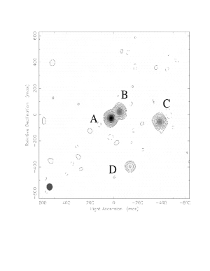
Figure 1: (LEFT) Example of an anomalous flux ratio. For a smooth potential we would expect the A and B images in B1555+375 to have the same flux (Marlow et al. 1999).
(RIGHT) ISM properties needed to explain anomalous flux ratios. For an optical depth function $\tau=\tau_{5}(\nu/5\hbox{GHz})^{\alpha}$ we show the estimated spectral index $\alpha$ as a function of the optical depth $\tau_{5}$ at 5 GHz for the radio lenses used in DK02 with published flux ratios at both 5 GHz and either 8 or 15 GHz. The points are coded by the image type: minima–squares, saddle points–triangles, brightest–filled, and faintest–open.

Our review of the problem will cover three basic topics. First, we will discuss the problem of distinguishing CDM substructure from other possible origins for the anomalous flux ratios. In particular, we introduce a simple statistical test for substructure in the gravity as compared to either propagation effects in the interstellar medium of the lens galaxy or poorly modeled contributions to the smooth gravitational potential of the lens galaxy. In §3 we review our estimate of the substructure mass fraction and its relation to simulations. Finally, in §4 we discuss the future of the method.

2 Testing for Substructure

Most of the existing studies of the anomalous flux ratio problem have focused on demonstrating that the problem can be explained by CDM substructure. The next problem is to demonstrate that they cannot be explained by other effects. We can divide the other possibilities into three categories. First, propagation effects in the interstellar medium of the lens galaxy could produce the observed anomalies. Second, the flux ratio anomalies could be created by problems in the models for the smooth potential of the primary lens. Third, we could be misinterpreting a microlensing effect created by the normal stellar populations of the lenses with the effects of more massive satellites. Since we will focus on radio lenses, where microlensing effects must be small because of the large source sizes (Koopmans & de Bruyn 2000), we will not discuss this effect in detail.

Here we explore the first two problems – distinguishing substructure from propagation effects or modeling errors. The first approach we could take is to argue individual cases. For example, almost all propagation effects should show a strong frequency dependence. One way to explore the required properties of the ISM is to assume an optical depth, $\tau=\tau_{5}(\nu/5\hbox{GHz})^{\alpha}$, for the radio lenses normalized by the optical depth $\tau_{5}$ at $5$ GHz and with a spectral index $\alpha$ for the frequency dependence. Fig. 1 shows the results of fitting such an ISM model to the radio lenses in DK02 where flux measurements were available at both 5 GHz and either 8 or 15 GHz. Common ISM effects, such as refractive scattering or free-free absorption, would show a spectral index of $\alpha\sim-2$, while the optical depth function needed to explain the data has almost no frequency dependence ($\alpha\simeq 0$). In short, explaining the anomalous flux ratios with the ISM requires the radio equivalent of the “gray dust” sometimes suggested to change the cosmological conclusions from Type Ia supernovae (Aguirre 1998).

Similarly, Metcalf & Zhao (2001), Keeton, Gaudi & Petters (2002) and Evans & Witt (2002) explore whether changes to the smooth potential can explain the problem. The basic result from these studies is that they cannot. Although Evans & Witt (2002) give an anti-substructure tenor to their results, we would argue that they have actually produced further arguments in favor of substructure. First, for the two lenses from DK02 they analyze, they can only explain the anomalous flux ratio of one system despite using lens models with essentially arbitrary angular structure. In fact, when we use similar models to analyze the full sample from DK02, we find that of the 6 systems (out of 7) which arguably have anomalous flux ratios, the more complicated models can successfully fit 2–3, at the price of having amplitudes for the higher order perturbations that are significantly larger than are generally observed for either the stars or in dark matter simulations. Second, the other two lenses Evans & Witt (2002) analyze are known from time variability studies to be microlensed (i.e. containing substructure but on a smaller mass scale), so the success of the Evans & Witt (2002) models at explaining the flux ratios in these systems shows that sufficiently complex macro models can mask the presence of substructure even when it is known to be present. This leaves us with a basic ambiguity of course, since standard models (ellipsoidal lens models combined with external tidal shear fields) cannot explain the anomalous flux ratios, while models with very complicated potentials can explain some, but not all, anomalous flux ratios, but can also do so in systems where they should not.

Fortunately, we need not live with these ambiguities, because low optical depth substructure has a unique property that allows us to statistically distinguish substructure from either the interstellar medium or problems in the smooth potential. The images of a lens can be assigned a parity depending on whether they are saddle points or minima of the virtual time delay surface (e.g. Schneider et al. 1992), and the four images alternate their parities as we go around the Einstein ring (saddle-minimum-saddle-minimum). Given a sample of lenses, we can divide the images into four separate classes (brightest saddle, faintest saddle, brightest minimum, faintest minimum) based on their parities and fluxes. As we now discuss, the effects of substructure depend on the image type, while the effects of the ISM and errors in the macro model generally do not.

Both microlensing by the stars (Schechter & Wambsganss 2002) and lensing by extended substructures (Keeton 2002) distinguishes between images based on their parities when the optical depth is low. The sense of the effect is to preferentially demagnify saddle points (negative total parity) compared to minima (positive total parity). The most magnified images are also affected more than the least magnified images because the high magnification makes them sensitive to smaller perturbations in the potential (Mao & Schneider 1998). We can study this effect by examining the distributions of the residuals, $\log(f_{obs}/f_{mod})$, between the model fluxes $f_{mod}$ and observed fluxes $f_{obs}$ for both the data and for different theories as to the origin of the anomalous flux ratios for the 4 different image types found in a quad lens (brightest saddle, faintest saddle, brightest minimum, faintest minimum). The top panel of Fig. 2 shows the distributions we find after fitting the 8 available radio quads using our standard model for the smooth potential (one or more singular isothermal ellipsoids in an external tidal shear field), and the middle panel shows the distribution predicted in a Monte Carlo simulation of a lens sample with a 5% substructure mass fraction. As expected from the previous theoretical studies, the simulation shows an offset of the distribution for the brightest saddle points from the distribution for the other images, in the sense of preferentially demagnifying the saddle point.

Figure 2: Residual distributions after fitting standard models. Each panel shows the integrated distributions of the flux residuals $\log(f_{obs}/f_{mod})$ given the observed $f_{obs}$ and best fitting model $f_{mod}$ image fluxes. The distributions are shown separately for the brightest (points) and faintest (no points) minima (solid lines) and saddle points (dashed lines). The top panel shows the distribution for the real data on 8 four-image radio lenses. The middle panel shows a Monte Carlo simulation of the distributions for lenses with a $f_{sat}=0.05$ mass fraction in substructure modeled as tidally truncated singular isothermal spheres. The lower panel shows a Monte Carlo simulation of the distributions for lenses with a large amplitude, randomly oriented $\cos 4\theta$ term in the gravitational potential of the lens that is not included in the lens model used to interpret the data. The mode amplitude of $a_{4}=0.05$ is the standard Fourier component used to analyze the photometry of elliptical galaxies. Note how the data (top) shows the same shift to fainter fluxes for the brightest saddle points as is expected from low optical depth substructure (middle), while an error in the macro model (bottom) does not distinguish between the image types.

The ISM, for example, makes a very different prediction. It is the clumpy, high density components of the ISM which will modify flux ratios, and this has two important consequences. First, propagation effects should preferentially modify the fluxes of the least magnified images, because they have the smallest intrinsic angular sizes. The more magnified images have larger angular sizes and will more effectively smooth out any effects of a clumpy ISM. Second, a clumpy ISM cannot distinguish between images of differing parities because the ISM properties are locally determined while the image parity is not – the magnification tensor depends on the projected surface density, the projected shear component of the gravity and the source and lens redshifts. Thus, in a statistical sample, the ISM might systematically perturb the fainter images more than the brighter images, but it will not distinguish between saddle points and minima.

The macro model also will have difficulty systematically perturbing images of a particular parity. Qualitatively this can be understood by the symmetry of merging image pairs from the point of view of the central potential – any slope in the curvature needed to produce a change in the magnification of the saddle point can just as easily appear with the opposite sign so as to produce the opposite change. While we lack a mathematical proof to this effect, it certainly holds in Monte Carlo simulations of lenses produced by potentials with complicated, higher order angular structures (as in Evans & Witt 2002) that are then modeled using standard ellipsoidal potentials. In Fig. 2 we show an example of the distribution of residuals expected for a population of lenses with a large, unmodeled $\cos 4\theta$ perturbation to the potential. Unlike the distributions expected for substructure shown in Fig. 2, we see that there is no distinction in the model residuals for the different images.

This then leads to a simple test for substructure – do the distributions of residuals from standard ellipsoidal models distinguish between the image types or do they not? We can immediately see the answer in Fig. 2 – the distribution of residuals for the brightest saddle point differs from that of the other three images just as expected for substructure. Quantitatively, the Kolmogorov-Smirnov test probability that the model residuals for the brightest saddle points have the same distribution as for the other images is $<0.1\%$. Other phrasings of the test, bootstrap resampling of the data, null tests with the image identifications randomly assigned all support the results that the statistical properties of the saddle points are fundamentally different from that of the other images. And this distinctiveness is the tell-tale sign that the anomalous flux ratios are due to substructure in the gravity rather than the ISM or problems in the smooth potential model for the lens galaxy.

3 Implications for CDM

If substructure is the explanation, then the next objective is to estimate the satellite mass fraction $f_{sat}$. Here we review the method and results of DK02. We modeled the substructure as tidally truncated singular isothermal spheres, with a critical radius scale $b=0\hbox{$.\!\!^{\prime\prime}$}001$ and a tidal radius $a=(bb_{0})^{1/2}$ where $b_{0}\simeq 1\hbox{$.\!\!^{\prime\prime}$}0$ is the critical radius of the primary lens galaxy. When the dominant effect of the substructure is to perturb magnifications rather than image positions, we can only measure the mass fraction $f_{sat}$ of the satellites with reasonable accuracy. The mass scale or mass function of the satellites is difficult to constrain unless there are significant astrometric perturbations. In outline, our approach was to take each lens and its standard model and then add random substructure realizations in order to determine the probability of finding an improved fit as a function of the parameters describing the substructure (principally the mass fraction, $f_{sat}$). Because the “macro” model for the smooth potential masks some of the effects of substructure, it is necessary to reoptimize the parameters of the “macro” model for every trial. We applied the method to a sample of 7 four-image lenses.

Figure 3: Monte Carlo simulations of the DK02 method. The left (right) panel shows the likelihood distributions for the substructure mass fraction produced by our method when $f_{sat}=0$ ($f_{sat}=0.05$). In the left panel, the dashed lines show the probabilities for the individual lenses and the solid lines show the joint likelihoods for two simulations of a sample of 7 lenses. For these simulations where the true $f_{sat}=0$, we find an upper bound of $f_{sat}\mathrel{\raise 1.29167pt\hbox{$<$}\mkern-14.0mu\lower 2.58334pt\hbox{$\sim$}}0.004$. In the right panel we show the joint likelihoods for eight simulations of a sample of 7 lenses (solid lines) in which the true substructure fraction is $f_{sat}=5\%$. The recovered satellite fractions are statistically consistent with the input fraction, albeit with broad uncertainties due to the small sample size. The heavy dashed line simulates a sample of 56 lenses (the product of all the solid lines), and the recovered value is slightly lower than the input value given the distribution width. The points on the curves indicate the median (triangles), 68% confidence (squares) and 95% confidence (pentagons) regions.

We can illustrate our method with Monte Carlo simulations. Fig. 3 shows the results for Monte Carlo simulations of our sample either with or without substructure. If we add no substructure, then we typically obtain an upper limit of $f_{sat}\mathrel{\raise 1.29167pt\hbox{$<$}\mkern-14.0mu\lower 2.58334pt\hbox{$\sim$}}0.004$ given the properties of our lens sample. This sets a lower limit for our detection threshold somewhat above the substructure fraction which would be associated with the visible satellites in the Galaxy. If we put $f_{sat}=0.05$ of the mass into substructure, then we recover the input fraction reasonably accurately. Of the eight Monte Carlo trials shown in Fig. 3, four agree with the input value to within the 68% ($1\sigma$) confidence region, and six agree to within the 90% confidence region. If we combine all 8 simulations into a synthetic sample of 56 lenses, we estimate that $f_{sat}=0.034$ with a 90% confidence range of $0.023\leq f_{sat}\leq 0.048$ that marginally excludes the true value. Similarly, if we attempt to recover the deflection scale of the substructure, the error bars are worse but the results do converge to the input value when we model a large enough sample of lenses.

Figure 4: Results for the DK02 sample of 7 lenses. The left panel shows the results for estimating $f_{sat}$ with $b=0\hbox{$.\!\!^{\prime\prime}$}001$ fixed, and the right panel shows the results estimating the deflection scale $b$ as well. Distributions are shown assuming flux measurement errors of 5%, 10% and 20%, where we adopted 10% as our standard estimate.

Fig. 4 shows the results for the real data. The biggest systematic uncertainty in the data is the level of systematic uncertainty in the flux ratio measurements, so we show the results for 5%, 10% and 20% uncertainties in flux measurements. We adopt 10% as our standard value – the measurements probably are not as accurate as 5%, they probably are more accurate than 10%, and they certainly are more accurate than 20%. With the 10% flux uncertainties we find a substructure fraction of $0.006\mathrel{\raise 1.29167pt\hbox{$<$}\mkern-14.0mu\lower 2.58334pt\hbox{$\sim$}}f_{sat}\mathrel{\raise 1.29167pt\hbox{$<$}\mkern-14.0mu\lower 2.58334pt\hbox{$\sim$}}0.07$ (90% confidence) that is in good agreement with the expectations for CDM models. We obtain a very poor estimate of the characteristic deflection scale, finding $0\hbox{$.\!\!^{\prime\prime}$}0001<b<0\hbox{$.\!\!^{\prime\prime}$}007$, which for a substructure mass function $dn/dM\propto M^{-1.7}$ implies an upper end to the substructure mass function of $10^{6}M_{\odot}$-$10^{9}M_{\odot}$ that is in crude accord with our expectations. The degenerate direction in the error contours of Fig. 4 correspond to keeping the magnification perturbations nearly constant while varying the astrometric perturbations.

4 In The Future

The future of the substructure question will be driven by further observations, both to clarify the origins of the anomalous flux ratios and to obtain improved estimates of the substructure mass fraction and mass function.

It is relatively straight forward to finish eliminating the ISM as a source of concern with new observations. In the radio this means measuring flux ratios at still higher frequencies (e.g. 43 GHz flux ratio measurements at the VLA) to constrain the frequency dependence of any propagation effect still more tightly. In the optical this means measuring flux ratios over long wavelength baselines to measure any dust extinction (e.g. Falco et al. 1999). Mid-infrared (5–10$\mu$m) flux ratios, where the wavelength is far to short to be bothered by electrons and far too long to be bothered by dust, are difficult to measure but completely insensitive to the ISM. Observations to find additional lensed structures in the systems with anomalous flux ratios are the best direct route to determining whether more complicated lens potentials are needed. In particular, very clean constraints on the strengths of any more complicated angular structure than is included in the standard ellipsoidal models can be obtained by analyzing the shapes of the Einstein ring images of the host galaxies (see Kochanek et al. 2001). Such data can be obtained for any lens through deep HST/NICMOS imaging of lens systems.

Improving estimates of the substructure parameters or the statistical case for (or against) substructure requires larger samples of lenses to include in the analysis. The primary problem in expanding the sample is the need to separate the effects of stars and satellites in the optically-selected lenses. The flux ratios of the optical quasars are affected by both substructure and stellar microlensing because the optical continuum emitting regions of accretion disks are so compact (see Schneider et al. (1992) for a general review of microlensing). By measuring the flux ratios of these lenses in either the mid-IR, where the emitting region is a large dust “torus,” or in the emission lines, where the emitting region is the relatively large broad/narrow emission line region, we can separate the effects of the stars from the effects of substructure (e.g. Moustakas & Metcalf 2002). While mid-IR imaging is difficult except for the brightest quasar lenses (see Agol et al. 2000), the advent of high spatial resolution integral field spectrographs on many 8m-class telescopes will make it relatively easy to measure emission line flux ratios.

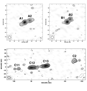
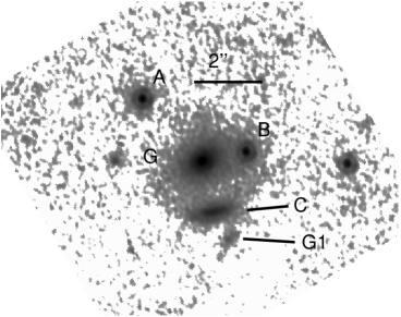
Figure 5: The Astrometric anomaly in MG2016+112. The left panels show the VLBI images from Koopmans et al. (2001) of the A, B and C images. The right panel shows the CASTLES HST/NICMOS H-band image of the system. For the same symmetry reasons that close image pairs should have the same fluxes, the C₁₁–C₁₂ and C₁₃–C₂ image separations should be the same. The fact that they differ is the astrometric equivalent of a flux anomaly. In this case it is created by the small galaxy G1 sitting to the South of the C images.

Our analysis methods also need to be improved. In particular, we need to properly treat the highest mass satellites, both to constrain the satellite mass function and to better estimate the mass fraction. In the DK02 analyses, we included the highest mass satellites as part of the macro model because they have such an enormous effect on the models that it is impossible to produce a reasonable model without including them. One example is the small satellite in MG0414+0534 (Object “X”; Schechter & Moore 1993), which at H-band has only 10% the luminosity of the main lens and in models has only 12% the critical radius of the main lens, but even when fitting only the positions of the quasar images produces a $\Delta\chi^{2}\simeq 100$ improvement in the fit once it is included (Ros et al. 2000).

We can also search for the astrometric equivalents of anomalous flux ratios so as to provide better constraints on the mass scale of the substructure (e.g Wambsganss & Paczynski 1992, Metcalf 2002). One example is the lens MG2016+112 (see Fig. 5) where in VLBI maps the C image is seen to be a pair of merging images each of which is composed of two VLBI components (Koopmans et al. 2001). For the same reasons that we would expect a merging image pair to have similar fluxes, we would expect them to have similar separations, so the very asymmetric separations of the VLBI components C₁₁–C₁₂ as compared to C₁₃–C₂ is the astrometric equivalent of an anomalous flux ratio. In this case, as in MG0414+0534, the culprit is a visible satellite G1 sitting to the south of the C image complex. It has only 1-2% the H-band luminosity and $\simeq 8\%$ the deflection scale of the main lens, and is known to lie at the same redshift as the lens galaxy. The VLBI data has sufficient resolution to detect a satellite with a deflection scale nearly 10 times smaller. The holy grail of searching for CDM substructure in gravitational lenses would be to find an astrometric anomaly similar to that in MG2016+112, so that there is compelling evidence for the existence of a satellite, but for which no luminous counterpart can be detected.

References

- (1) Agol, E., Jones, B., & Blaes, O., 2000, ApJ, 545, 657
- (2) Aguirre, A. N. 1998, ApJ, 512, L19
- (3) Avila-Reese, V., Colín, P., Valenzuela, O., D’Onghia, E., & Firmani, C. 2001, ApJ, 559, 516
- (4) Bode, P., Ostriker, J. P., & Turok, N. 2001, ApJ, 556, 93
- (5) Bradac, M., Schneider, P., Steinmetz, M., Lombardi, M., & King, L.J., 2002, A&A, 388, 373
- (6) Bullock, J. S., Kravtsov, A. V., & Weinberg, D. H. 2000, ApJ, 539, 517
- (7) Chiba, M. 2002, ApJ, 565, 17
- (8) Colín, P., Avila-Reese, V., & Valenzuela, O. 2000, ApJ, 542, 622
- (9) Colín, P., Avila-Reese, V., Valenzuela, O., & Firmani, C. 2002, astro-ph/0205322
- (10) Dalal, N. & Kochanek, C. S. 2002, ApJ, 572, 25 [DK02]
- (11) D’Onghia, E. & Burkert, A. 2002, astro-ph/0206125
- (12) Evans, N. W. & Witt, H. J. 2002, astro-ph/0212013
- (13) Falco, E. E. et al. 1999, ApJ, 523, 617
- (14) Kamionkowski, M. & Liddle, A. R. 2000, Physical Review Letters, 84, 4525
- (15) Kauffmann, G., White, S.D.M., & Guiderdoni, B., 1993, MNRAS, 264, 201
- (16) Keeton, C. R. 2001a, astro-ph/0111595
- (17) Keeton, C. R. 2002, astro-ph/0209040
- (18) Keeton, C.R., Gaudi, B.S., & Petters, A.O., 2002, ApJ submitted, astro-ph/0210318
- (19) Klypin, A., Kravtsov, A.V., Valenzuela, O., & Prada, F., 1999, ApJ, 522, 82.
- (20) Kochanek, C. S., Keeton, C. R., & McLeod, B. A. 2001, ApJ, 547, 50
- (21) Koopmans, L. V. E. and de Bruyn, A. G. 2000, A&A, 358, 793
- (22) Koopmans, L. V. E., Garrett, M. A., Blandford, R. D., et al., Porcas, R. W. 2002, MNRAS, 334, 39
- (23) Mao, S., & Schneider, P., 1998, MNRAS, 295, 587
- (24) Marlow, D.R., Myers, S.T., Rusin, D., et al., 1999, AJ, 118, 654
- (25) Metcalf, R. B. & Madau, P. 2001, ApJ, 563, 9
- (26) Metcalf, R. B. and Zhao, H. 2002, ApJ, 567, L5
- (27) Metcalf, R. B., 2002, ApJ, 580, 696
- (28) Moore, B. Ghigna, S., Governato, F., et al., 1999, ApJ, 524, L19
- (29) Moustakas, L. A. & Metcalf, R. B. 2002, astro-ph/0203012
- (30) Ros., E., Guirado, J.C., Marcaide, J.M., et al., 2000, A&A, 362, 845
- (31) Schechter, P. L. & Moore, C. B. 1993, AJ, 105, 1
- (32) Schechter, P. L. & Wambsganss, J. 2002, astro-ph/0202425
- (33) Schneider, P., Ehlers, J., & Falco, E.E., 1992, Gravitational Lenses, (Springer Verlag: Berlin)
- (34) Spergel, D. N. & Steinhardt, P. J. 2000, Physical Review Letters, 84, 3760
- (35) Wambsganss, J., & Paczynski, B., 1992, ApJ, 397, L1
- (36) Yoshida, N., Springel, V., White, S. D. M., & Tormen, G. 2000, ApJ, 544, L87