Mapping the 3-D Dark Matter Potential with Weak Shear

Abstract

We investigate the practical implementation of Taylor’s (2002) 3-dimensional gravitational potential reconstruction method using weak gravitational lensing, together with the requisite reconstruction of the lensing potential. This methodology calculates the 3-D gravitational potential given a knowledge of shear estimates and redshifts for a set of galaxies. We analytically estimate the noise expected in the reconstructed gravitational field taking into account the uncertainties associated with a finite survey, photometric redshift uncertainty, redshift-space distortions, and multiple scattering events. In order to implement this approach for future data analysis, we simulate the lensing distortion fields due to various mass distributions. We create catalogues of galaxies sampling this distortion in three dimensions, with realistic spatial distribution and intrinsic ellipticity for both ground-based and space-based surveys. Using the resulting catalogues of galaxy position and shear, we demonstrate that it is possible to reconstruct the lensing and gravitational potentials with our method. For example, we demonstrate that a typical ground-based shear survey with redshift limit $z=1$ and photometric redshifts with error $\Delta z=0.05$ is directly able to measure the 3-D gravitational potential for mass concentrations $\ga 10^{14}M_{\odot}$ between $0.1\la z\la 0.5$, and can statistically measure the potential at much lower mass limits. The intrinsic ellipticity of objects is found to be a serious source of noise for the gravitational potential, which can be overcome by Wiener filtering or examining the potential statistically over many fields. We examine the use of the 3-D lensing potential to measure mass and position of clusters in 3-D, and to detect clusters behind clusters.

1 Introduction

Gravitational lensing affords us a direct method to probe the distribution of matter in the universe, irrespective of its state or nature. This deflection of light by the gravitational potential of matter along its path can be observed as a local alteration of number counts of background galaxies (magnification), or a distortion of their shape (shear). It is the latter phenomenon which we will concern ourselves with here; we will further restrict ourselves to the case where this distortion is weak ($\la 10$% change in the ellipticity of the object). Despite the weakness of the effect, and the intrinsic, nearly randomly orientated ellipticity of background galaxies, we can measure the weak shear by averaging the ellipticity or shear estimates of very many galaxies.

It has long been recognised that weak gravitational lensing is a valuable tool for examining the two dimensional projected matter distribution, and can consequently provide important information regarding large-scale structure (see e.g. Bartelmann & Schneider 2000, Bernardeau et al 1997, Jain & Seljak 1997, Kaiser 1998). In particular, the sensitivity of lensing to all the matter present, including the dominant dark matter, ensures that the weak lensing effect is an excellent probe for determining the quantity and distribution of matter.

Weak lensing studies for a wide range of galaxy clusters have been carried out, allowing precision measurements of the clusters’ masses and mass distributions (see e.g. Tyson et al 1990, Kaiser & Squires 1993, Bonnet et al 1994, Squires et al 1996, Hoekstra et al 1998, Luppino & Kaiser 1997, Gray et al 2002). Moving to larger scales, the shear due to large-scale structure has been accurately measured by several groups (see e.g. van Waerbeke et al 2001, Hoekstra et al 2002, Bacon et al 2002, Refregier et al 2002, Brown et al 2002).

Redshift information has already been used in weak lensing studies, e.g. to determine the median redshifts of the lens and background populations; most analyses then project the lensing information into a 2-dimensional projected mass distribution. Wittman et al (2001, 2002) demonstrate the utility of using 3-D shear information by inferring the redshift of a cluster using shear and photometric redshift information for the galaxies in their sample. The importance of including redshift information to remove intrinsic galaxy alignments from shear studies has also been discussed (Heymans & Heavens 2002, King & Schneider 2002a,b). Lens tomography has been studied as a valuable means of introducing redshift information into shear power spectra (e.g. Seljak 1998, Hu 1999, 2002, Huterer 2002, King & Schneider 2002b), but only recently has the full reconstruction of the 3-D Dark Matter distribution from lensing been considered (Taylor 2002, Hu & Keaton 2002).

In this paper, we seek to discuss a practical implementation for reconstruction of the 3-D lensing and gravitational potentials from weak lensing measurements and redshift information (whether photometric or spectroscopic). We will use the reconstruction procedure of Taylor (2002), which allows us to calculate the entire 3-D gravitational potential if we have a knowledge of shear estimates and redshifts for a set of galaxies. This procedure is explained in Section 2.

In Section 3 we discuss sources of uncertainty for our reconstruction, examining analytically the effect of shot noise due to galaxy ellipticity, the effects induced by a finite survey, photometric redshift errors, redshift-space distortions, and multiple scatterings of light rays.

We aim to test the reconstruction method using simulations of realistic weak lensing data. In practice, for a particular volume of space containing a mass distribution, the data which would result from a real survey would be a set of galaxy ellipticities (in the weak lensing regime, these will be dominated by intrinsic ellipticity with a small gravitational lensing perturbation) and redshifts. The ellipticities will typically be defined by the galaxies’ quadrupole moments (e.g. Kaiser et al 1995, Rhodes et al 2000) or estimated from a decomposition of galaxy shape into eigenfunctions (Refregier & Bacon 2002, Bernstein & Jarvis 2002). In order to provide a realistic catalogue of these data, we simulate mass distributions, calculate the expected lensing distortion in 3-D, and create a set of galaxies probing this distortion with a realistic redshift distribution and intrinsic ellipticity. We describe this procedure in detail in Section 4.1.

Given such a catalogue, we attempt to reconstruct the lensing potential and gravitational potential (Section 4.2). We use a generalised 3-D Kaiser-Squires (1993) inversion together with Taylor’s (2002) formalism to obtain the 3-dimensional gravitational potential distribution.

In Section 5 we demonstrate the effectiveness of our implementation in reconstructing lensing and gravitational potentials. We examine the level of noise in our simulations in Section 6, including the Poisson noise associated with having only a finite number of galaxies probing the lensing distribution, and the noise from galaxies’ intrinsic ellipticities. We go on to examine the uncertainties caused by photometric or spectroscopic redshift errors.

In Section 7 we study the utility of reconstructing only the 3-D lensing potential without continuing to the gravitational potential; this provides a useful method for detecting mass concentrations and measuring their mass and 3-D position. Finally, we summarise our results in Section 8.

2 3-D Gravitational Potential Reconstruction

In this section we will summarise the results of Taylor’s (2002) approach to reconstructing the 3-D gravitational potential, using weak lensing measurements together with redshifts for all galaxies in the lensing catalogue.

We begin by noting that the Newtonian gravitational potential $\Phi$ can be related to the density of matter $\rho$ by Poisson’s equation,

$$\nabla^{2}\Phi=4\pi G\rho_{m}\delta a^{2}=\frac{3}{2}\lambda_{H}^{-2}\Omega_{m}a^{-1}\delta,$$ (1)

where we have introduced the cosmological scale factor $a$, the density contrast $\delta=(\rho-\bar{\rho})/\bar{\rho}$, the Hubble length $\lambda_{H}=1/H_{0}\approx 3000\,h^{-1}{\rm Mpc}$, and the present-day mass-density parameter $\Omega_{m}$.

We can study the impact of this gravitational potential on image distortion due to gravitational lensing, by introducing the lensing potential $\phi$. This is a measure of the distortion which is related to the observable shear matrix by

$$\gamma_{ij}=\left(\partial_{i}\partial_{j}-\frac{1}{2}\delta^{K}_{ij}\partial^{2}\right)\phi,$$ (2)

where $\partial_{i}\equiv r(\delta_{ij}-\hat{r}_{i}\hat{r}_{j})\nabla_{j}=r(\nabla_{i}-\hat{r}_{i}\partial_{r})$ is a dimensionless, transverse differential operator, and $\partial^{2}\equiv\partial_{i}\partial^{i}$ is the transverse Laplacian. The indices $(i,j)$ take the values $(1,2)$, and we have assumed a flat sky.

The lensing potential is also observable via the lens convergence field

$$\kappa=\frac{1}{2}\partial^{2}\phi.$$ (3)

The convergence field is related to the shear field by the differential relation, first used by Kaiser & Squires (1993);

$$\kappa=\partial^{-2}\partial_{i}\partial_{j}\gamma_{ij},$$ (4)

where $\partial^{-2}$ is the inverse 2-D Laplacian operator on a flat sky, defined by

$$\partial^{-2}\equiv\frac{1}{2\pi}\int\!d^{2}\!\theta\,\ln|\mbox{\boldmath$\theta$}-\mbox{\boldmath$\theta$}^{\prime}|.$$ (5)

Note that transverse positions $\theta$ in this equation will be quoted in units of radians, so that the lensing quantities are dimensionless. However, such angular positions can be arbitrarily scaled, leading to simple scalings on the lensing quantities which we will quote later.

A useful quantity for tracing noise and systematics in gravitational lensing is the divergence-free field, $\beta$, defined by

$$\beta=\partial^{-2}\varepsilon^{n}_{i}\partial_{j}\partial_{n}\gamma_{ij},$$ (6)

where $\epsilon^{n}_{i}=\left(\begin{array}[]{c c}0&-1\\ 1&0\end{array}\right)$. If $\gamma_{ij}$ is generated purely by the lensing potential, $\beta$ vanishes. But if there are non-potential sources, due to noise, systematics or intrinsic alignments, then $\beta$ will be non-zero. In addition, $\beta$ terms can arise from finite fields, due to mode-mixing of shear fields (e.g. Bunn 2002). We discuss this further in Section 3.2.

We can relate the lensing potential and the gravitational potential by

$$\phi(\mbox{\boldmath$r$})=2\int_{0}^{r}\!\!dr^{\prime}\,\left(\frac{r-r^{\prime}}{rr^{\prime}}\right)\Phi(\mbox{\boldmath$r$}^{\prime}),$$ (7)

in a spatially flat universe, with comoving distance $r$. This equation assumes the Born approximation, in which the path of integration is unperturbed by the lens.

Note that the lensing potential is really a 3-D quantity, although usually it is regarded as a 2-D variable in the absence of redshift information. In this case the usual practice is to average over the redshift distribution of the source galaxies (e.g. Bartelmann & Schneider 2001). It is in this 2-D approximation that the depth information is lost in lensing.

Given that $\phi(\mbox{\boldmath$r$})$ is really a 3-D variable, we can readily, and exactly, invert equation (7) and recover the full 3-D Newtonian potential (Taylor 2002);

$$\Phi(\mbox{\boldmath$r$})=\frac{1}{2}\partial_{r}r^{2}\partial_{r}\,\phi(\mbox{\boldmath$r$})$$ (8)

where $\partial_{r}=\hat{\mbox{\boldmath$r$}}.\nabla$ is the radial derivative. Any lensing field from real data will contain significant noise, and will thus require smoothing if we are to perform this differentiation. Interestingly it turns out that the lensing potential obeys a second-order differential equation, which is $r^{2}$ times the radial part of the 3-D Laplacian. This appears to be just a coincidence given that the lensing kernel in equation (7) is solely due to the geometric properties of the lens.

In order to reconstruct the gravitational potential, it is necessary to find the lensing potential from the shear. This can be achieved by using the Kaiser-Squires (1993) relation, generalised to 3-D:

$$\widehat{\phi}(\mbox{\boldmath$r$})=2\partial^{-4}\partial_{i}\partial_{j}\ \gamma_{ij}(\mbox{\boldmath$r$}),$$ (9)

where $\widehat{\phi}$ is an estimate of $\phi$. As the variance of the shear field is formally infinite (Kaiser & Squires 1993), this distribution is usually binned and/or smoothed in the transverse direction before calculating the lensing potential.

The above solution allows us to estimate the lensing potential only up to an arbitrary function of the radial distance $r$:

$$\widehat{\phi}(\mbox{\boldmath$r$})=\phi(\mbox{\boldmath$r$})+\psi(r),$$ (10)

where $\phi$ is the true lensing potential, and $\psi(r)$ is a solution to

$$\left(\partial_{i}\partial_{j}-\frac{1}{2}\delta^{K}_{ij}\partial^{2}\right)\psi=0.$$ (11)

This arbitrary radial behaviour is due to the fact that the shear only defines the lensing potential up to a constant for each slice in depth. However, we must tame this behaviour if we wish to apply equation (8) to find the gravitational potential.

Fortunately, there are several opportunities for removing $\psi$. Firstly, since $\langle\phi\rangle=0$ for each slice in depth from homogeneity and isotropy conditions, we can simply subtract $\langle\widehat{\phi}\rangle$ from $\widehat{\phi}$ for each radial slice, provided that our survey is large enough to discount errors in $\langle\phi\rangle$. Thus

$$\Phi=\frac{1}{2}\partial_{r}r^{2}\partial_{r}(\widehat{\phi}-\langle\widehat{\phi}\rangle).$$ (12)

Alternatively, we can note that $\langle\partial_{r}\phi\rangle=0$ for each radial slice, with a similar subtraction required. Given these procedures, it is clear that $\psi$ can be removed for large surveys, where the necessary averages $\langle\tilde{\phi}\rangle$ or $\langle\partial_{r}\tilde{\phi}\rangle$ will have small uncertainty; however for limited area surveys $\psi$ will not be estimated well, leading to uncertainties on the reconstruction (see Section 3.1.2).

Similar relationships between the potential and the 3-D lens convergence can also be written down:

$$\Phi=\partial_{r}r^{2}\partial_{r}(\partial^{-2}\kappa-\langle\partial^{-2}\kappa\rangle),$$ (13)

while the relationship between the matter density field and the 3-D convergence is

$$\delta=\left(\frac{2\lambda_{H}^{2}a}{3\Omega_{m}}\right)\nabla^{2}\partial_{r}r^{2}\partial_{r}(\partial^{-2}\kappa-\langle\partial^{-2}\kappa\rangle).$$ (14)

With these sets of equations, the 3-D lensing convergence, 3-D lensing potential, 3-D Newtonian potential and 3-D matter density fields can all be generated from combined shear and redshift information.

3 The uncertainty in 3-D lensing

3.1 Shot-noise uncertainty in lensing fields

Having written down the basic equations for the 3-D analysis of gravitational lensing data, we now consider the various contributions to the uncertainty in a reconstruction of these fields.

3.1.1 The convergence field

The covariance on a reconstructed, continuous convergence field due to shot-noise is generally given by

$$\langle\kappa(\mbox{\boldmath$r$})\kappa(\mbox{\boldmath$r$}^{\prime})\rangle_{SN}=\frac{\gamma^{2}_{\rm rms}}{n(\mbox{\boldmath$r$})}\delta_{D}(\mbox{\boldmath$r$}-\mbox{\boldmath$r$}^{\prime}),$$ (15)

where $\gamma_{\rm rms}$ is the intrinsic dispersion of galaxy shear estimates in one component (i.e. $\gamma_{1}$ or $\gamma_{2}$) due to the non-circularity of galaxies, and $n(\mbox{\boldmath$r$})$ is the observed space density of galaxies in a survey.

In the case of a discretised map this reduces to

$$\langle\kappa_{i}\kappa_{j}\rangle_{SN}=\frac{\gamma^{2}_{\rm rms}}{N_{pix}}\delta^{K}_{ij},$$ (16)

where, for a constant 3-D number density of galaxies,

$$N_{pix}=3\bar{n}\theta_{pix}^{2}r^{2}\Delta r/R^{3}$$ (17)

is the 3-D pixel occupation number, $\bar{n}$ is the 3-D density of galaxies, $\theta_{pix}$ is the pixel size, $\Delta r$ is the width of the radial bins, $r$ is the radial distance, and $R$ is the chosen limiting distance for the survey. We will compare this amplitude and behaviour with our simulations in Section 6.

3.1.2 The lensing potential field

We now wish to describe the uncertainty expected for the lensing potential field. We can write the covariance of the lensing potential estimated from equation (3) as

$$\langle\phi(\mbox{\boldmath$r$})\phi(\mbox{\boldmath$r$}^{\prime})\rangle_{SN}=4\partial^{-2}\partial^{\prime-2}\langle\kappa(\mbox{\boldmath$r$})\kappa(\mbox{\boldmath$r$}^{\prime})\rangle_{SN}.$$ (18)

We describe the procedure used to evaluate this covariance in the Appendix, and here only quote the resulting variance of the lensing potential at the centre of the survey ($\mbox{\boldmath$\theta$}=0$) as a function of survey size, $\theta$, and radial position, $r$, in the flat-sky limit:

$$\langle\Delta\phi^{2}(\mbox{\boldmath$\theta$}=0)\rangle_{SN}=\frac{5}{24\pi}\frac{\gamma^{2}_{\rm rms}}{n(r)}\frac{\theta^{2}}{r^{2}}\delta_{D}(r-r^{\prime}).$$ (19)

Note that the uncertainty on the potential difference increases with the survey area as a consequence of the 2-D flat-sky lensing “force” term, $\ln|\mbox{\boldmath$\theta$}-\mbox{\boldmath$\theta$}^{\prime}|$, increasing with distance. We will compare this behaviour with our simulations in Section 6.

Finally we can cast this in a more convenient form for gravitational lensing in the discrete case:

$$\langle\Delta\phi^{2}(0)\rangle_{SN}=7.6\times 10^{-16}\left(\frac{n_{2}}{30/[1^{\prime}]^{2}}\right)^{-1}\left(\frac{\theta}{1^{\circ}}\right)^{2}\left(\frac{R^{3}}{r^{2}\Delta r}\right),$$ (20)

where we have assumed $\gamma_{\rm rms}=0.2$, $n_{2}=\frac{1}{3}nR^{3}$ is the 2-D total surface density of galaxies and $R$ is the nominal depth of the survey.

In general the uncertainty in the 3-D lensing potential will also depend on the pixel size as well as the total size of the survey. This behaviour for the uncertainty on the lensing potential is now due to the 2-D flat-sky lensing “force” term diverging at small separation. Due to the complexity of analysing this effect analytically we shall defer a more thorough treatment of studying pixelisation effects with our simulations to Section 6.

3.1.3 The Newtonian potential field

We also wish to calculate the uncertainty on the 3-D Newtonian potential. We can approach this, from equation (8), by differentiating the lensing potential field leading in the far-field limit to

$$\langle\Phi(\mbox{\boldmath$r$})\Phi(\mbox{\boldmath$r$}^{\prime})\rangle_{SN}=\frac{1}{4}r^{2}r^{\prime 2}\partial_{r}^{2}\partial_{r}^{\prime 2}\langle\phi(\mbox{\boldmath$r$})\phi(\mbox{\boldmath$r$}^{\prime})\rangle_{SN}.$$ (21)

We again describe the detailed calculation of this quantity in the Appendix, where we arrive at an expression for the variance on the Newtonian potential:

$$\langle\Phi^{2}(r)\rangle_{SN}=\frac{5}{64\pi\sqrt{2\pi}}\frac{\gamma^{2}_{\rm rms}}{r_{||}^{3}n}\left(\frac{r}{r_{||}}\right)^{4}\left(\frac{r_{||}}{R}\right)^{2}\theta^{2},$$ (22)

where $r_{||}$ is the smoothing radius for a radial Gaussian smoothing of the field. Hence we find that the shot-noise uncertainty is a strong function of the radial smoothing, changing as the inverse fifth power of the smoothing radius. We will again examine this behaviour in our simulations in Section 6.

Finally, we can again cast this in a more convenient form for lensing:

$$\langle\Phi^{2}(r)\rangle_{SN}=1.1\times 10^{-16}\left(\frac{n_{2}}{30/[1^{\prime}]^{2}}\right)^{-1}\left(\frac{\theta}{1^{\circ}}\right)^{2}\left(\frac{r}{r_{||}}\right)^{4}\left(\frac{R}{r_{||}}\right).$$ (23)

Note that, as for the lensing potential, the error upon the gravitational potential grows with survey or cell size.

The question of what survey area and radial smoothing to choose leaves us with an optimisation problem. From equation (22) it would appear that we can reduce the shot-noise by reducing the survey area, or increasing the radial smoothing. However the latter will reduce the resolution of the survey, and correspondingly lower the intrinsic signal, while the former will increase the noise effects induced by a finite survey area. We shall investigate further the effects arising from a finite survey in Section 3.2, and comment further on the problem of survey optimisation.

3.1.4 The density field

Finally the shot-noise uncertainty in the reconstructed density field can be constructed from equation (1);

$$\langle\delta(\mbox{\boldmath$r$})\delta(\mbox{\boldmath$r$}^{\prime})\rangle=\left(\frac{2\lambda_{H}^{2}a}{3\Omega_{m}}\right)^{2}\nabla^{2}\nabla^{\prime 2}\langle\Phi(\mbox{\boldmath$r$})\Phi(\mbox{\boldmath$r$}^{\prime})\rangle.$$ (24)

In the far-field approximation the Laplacian can be written $\nabla^{2}=(\partial_{r}^{2}+R^{-2}\partial^{2})$. In general equation (24) must be calculated numerically, but for points along the centre of the survey the shot-noise contribution to the variance of the density field can be calculated analytically, reducing to

$$\langle\delta^{2}(r)\rangle_{SN} = \left(\frac{2}{9\pi^{3}}\right)^{\frac{1}{2}}\left(\frac{a}{\Omega_{m}}\right)^{2}\frac{\gamma_{\rm rms}^{2}}{nr_{||}^{3}}\left(\frac{\lambda_{H}}{R}\right)^{4}\left(\frac{r^{2}}{r_{||}\theta R}\right)^{2}$$ (25)

$$\times\left[1+\frac{175}{24}\left(\frac{\theta R}{r_{||}}\right)^{4}\right].$$

If we set $a=1/2$, and $\gamma_{\rm rms}=0.2$, and again define $n_{2}=\frac{1}{3}nR^{3}$ as the surface galaxy density, the variance of the density field can be expressed in the form

$$\langle\delta^{2}(r)\rangle_{SN} = 2.9\times 10^{-8}\left(\frac{\Omega_{m}}{0.3}\right)^{-2}\left(\frac{n_{2}}{[30/1^{\prime}]^{2}}\right)^{-1}\left(\frac{\theta}{1^{\circ}}\right)^{-2}$$

$$\times \!\!\!\!\!\!\left(\frac{\lambda_{H}}{r_{||}}\right)^{4}\left(\frac{r^{4}}{r_{||}R^{3}}\right)\left[1+6.8\times 10^{-7}\left(\frac{(\theta/1^{\circ})R}{r_{||}}\right)^{4}\right],$$

To illustrate this we find that the variance in the reconstructed density field for $r_{||}=0.1$, $R=1$ and $r=1$, where we express distances here in redshift for a Euclidean universe, with $n_{2}=30$ galaxies per sq. arcmin. and $\Omega_{m}=0.3$ is given by

$$\langle\delta^{2}(r)\rangle_{SN}=0.003\left(\frac{\theta}{1^{\circ}}\right)^{-2}\left[1+0.007\left(\frac{\theta}{1^{\circ}}\right)^{4}\right],$$ (27)

which has a minimum at $\theta=3.2^{\circ}$ of $\langle\delta^{2}\rangle^{1/2}=0.02$. Since we expect the amplitude of density perturbations on these scales, $\lambda\approx 100\,h^{-1}{\rm Mpc}$, to be smaller than this, $\sigma_{\delta}\approx 0.01$, we can expect that filtering (e.g. Wiener filtering, see Section 3.3) will be required to extract a large-scale map of the 3-D density field, even at the scale which minimises noise.

3.2 Uncertainty and mode-mixing due to finite fields

3.2.1 Finite surveys

As well as shot-noise arising from the discrete sampling of the shear field by the survey galaxies, there is an additional uncertainty in the reconstruction of the density field for finite area surveys due to the reconstruction process being nonlocal (via the inverse Laplacian). The nonlocal behaviour of density reconstruction over a finite survey area also gives rise to a mixing of modes. Here we try to quantify for the first time for lensing the effects of mode-mixing and reconstruction noise arising from finite survey areas. The following analysis will be applicable to either 3-D or 2-D lensing studies, as the results will be true for either a series of redshift slices or an overall 2-dimensional projection.

We may calculate the effect of a finite shear sample by multiplying the shear field by an arbitrary window function;

$$\gamma^{\prime}_{ij}(\mbox{\boldmath$r$})=W(\mbox{\boldmath$r$})\gamma_{ij}(\mbox{\boldmath$r$}).$$ (28)

The lens convergence field can be estimated via equation (4), but since here there is only a finite field to integrate over, the effect of the window function is to truncate the effects due to the distant shear field and induce mode-mixing between $\kappa$ and $\beta$.

If we expand the shear in Fourier modes on the flat sky, the observed shear is a convolution of the intrinsic shear and the window function. For convenience we shall use continuous transforms, although for a finite sky a discrete Fourier transform with suitable boundary conditions is more practical. A scalar quantity $f(\mbox{\boldmath$\theta$},r)$ can be expanded in a 2-D Fourier series by

$$f(\mbox{\boldmath$\theta$},r)=\int\!\frac{d^{2}\ell}{(2\pi)^{2}}\,f(\mbox{\boldmath$\ell$},r)e^{i\mbox{\boldmath$\ell$}.\mbox{\boldmath$\theta$}}.$$ (29)

Decomposing the observed shear matrix given by equation (28) into the Fourier decomposed $\kappa(\mbox{\boldmath$\ell$})$ and $\beta(\mbox{\boldmath$\ell$})$ fields using equations (4) and (6), and Fourier transforming again we find the relationships between the reconstructed and true $\kappa$- and $\beta$-modes are

$$\kappa^{\prime}(\mbox{\boldmath$\ell$})\!\!\!\! = \!\!\!\!\int\!\frac{d^{2}\ell^{\prime}}{(2\pi)^{2}}\,W(\mbox{\boldmath$\ell$}-\mbox{\boldmath$\ell$}^{\prime})[\kappa(\mbox{\boldmath$\ell$}^{\prime})\cos 2\varphi-\beta(\mbox{\boldmath$\ell$}^{\prime})\sin 2\varphi],$$

$$\beta^{\prime}(\mbox{\boldmath$\ell$})\!\!\!\! = \!\!\!\!\int\!\frac{d^{2}\ell^{\prime}}{(2\pi)^{2}}\,W(\mbox{\boldmath$\ell$}-\mbox{\boldmath$\ell$}^{\prime})[\beta(\mbox{\boldmath$\ell$}^{\prime})\cos 2\varphi+\kappa(\mbox{\boldmath$\ell$}^{\prime})\sin 2\varphi],$$ (30)

where $\cos\varphi=\mbox{\boldmath$\hat{\ell}$}.\mbox{\boldmath$\hat{\ell}$}^{\prime}$. Hence we see that a finite survey will give rise to a spurious $\beta$-field. Here we have suppressed the radial dependence for clarity, so these equations are directly applicable to reconstruction of the convergence field in 2-D lensing.

If we assume negligible intrinsic $\beta$ fields then the real-space convergence is given by

$$\kappa^{\prime}(\mbox{\boldmath$\theta$})=\int\!\frac{d^{2}\ell}{(2\pi)^{2}}\kappa(\mbox{\boldmath$\ell$})\widetilde{W}_{\ell}(\mbox{\boldmath$\theta$})e^{-\ell^{2}\theta_{s}^{2}/2},$$ (31)

where

$$\widetilde{W}_{\ell}(\mbox{\boldmath$\theta$})=\int\!\frac{d^{2}\ell^{\prime}}{(2\pi)^{2}}W(\mbox{\boldmath$\ell$}-\mbox{\boldmath$\ell$}^{\prime})\cos 2\varphi\,e^{i\mbox{\boldmath$\ell$}^{\prime}.\mbox{\boldmath$\theta$}}$$ (32)

is the total effect of the finite survey area, and we have assumed the shear field is Gaussian smoothed on a scale $\theta_{s}$.

3.2.2 Variance of the convergence field

The variance measured in the finite-survey convergence field on a smoothing scale of $\theta_{s}$ is given by

$$\langle\kappa^{\prime 2}(\mbox{\boldmath$\theta$})\rangle=\int\!\frac{d^{2}\ell}{(2\pi)^{2}}C_{\ell}^{\kappa\kappa}|\widetilde{W}_{\ell}(\mbox{\boldmath$\theta$})|^{2}e^{\ell^{2}\theta_{s}^{2}},$$ (33)

where

$$\langle X(\mbox{\boldmath$\ell$})Y(\mbox{\boldmath$\ell$})\rangle=(2\pi)^{2}C^{XY}_{\ell}\delta_{D}(\mbox{\boldmath$\ell$}-\mbox{\boldmath$\ell$}^{\prime})$$ (34)

for the isotropic fields $X(\mbox{\boldmath$\theta$})$ and $Y(\mbox{\boldmath$\theta$})$.

If we approximate the window function by a Gaussian of radius $\theta$ with Fourier transform

$$W(\ell)=2\pi\theta^{2}\exp(-\ell^{2}/2\theta^{2}),$$ (35)

we can evaluate $\widetilde{W}_{\ell}(\mbox{\boldmath$\theta$})$ at $\mbox{\boldmath$\theta$}=0$, yielding

$$\widetilde{W}_{\ell}(0)=1+\frac{2(e^{-\ell^{2}\theta^{2}/2}-1)}{\ell^{2}\theta^{2}}.$$ (36)

Figure 1: The finite-field lensing window function, $\widetilde{W}_{\ell}(0)$, for a Gaussian window of radius $\theta$, calculated at the centre of the survey as a function of $\ell\theta$.

We plot this window function, giving the contribution of convergence modes to the observed convergence, in Figure 1. The general effect of the window function is to act as a high-pass filter. At $\ell\sim 1/\theta$ all the convergence modes are destroyed, while at large $\ell\theta$ the window function tends to unity as all the modes on scales below the scale of the survey contribute to the variance. Interestingly at low $\ell\theta$ this function goes negative, indicating that modes larger than the survey area are heavily distorted.

For the Gaussian window function, no $\beta$-modes are generated at the centre of the field due to the symmetry of the window. Hence the $\beta$-modes that are generated by the finite window are distributed nonlocally over the survey area.

Figure 2: Variance of reconstructed convergence field, $\kappa^{\prime}$, Gaussian smoothed on a scale $\theta_{s}=0.05^{\circ}$, measured at centre of Gaussian survey, as a function of survey radius, $\theta$ (solid line). The variance in the reconstructed convergence due to shear structure beyond the survey boundary is also shown (dotted line).

Figure 2 shows the variance of the observed convergence field, $\kappa^{\prime}$, on a smoothing scale of $\theta_{s}=0.05^{\circ}$, measured at the centre of a Gaussian survey as a function of the survey radius, $\theta$ (solid line). We have assumed a convergence power spectrum, $C^{\kappa\kappa}_{\ell}$, for a flat LCDM universe with $\Omega_{m}=0.3$, $\Omega_{\Lambda}=0.7$ and used the Peacock-Dodds transformation (Peacock & Dodds 1996) to map to the nonlinear regime. Below a survey radius of $\theta=0.1$ deg., missing modes due to the finite window and mode-mixing result in a drop in the measured variance.

3.2.3 Uncertainty in the reconstructed convergence

In addition to estimating the variance in the reconstructed convergence field $\langle\kappa^{\prime}(\mbox{\boldmath$\theta$})\rangle_{\rm obs}$ measured from within a finite survey, we can also predict the uncertainty $\langle\kappa^{\prime}(\mbox{\boldmath$\theta$})\rangle_{\rm miss}$ due to missing structure in the shear field beyond the survey area. As the total variance measured within the survey and the missing modes from beyond the survey must yield the total variance of the convergence field $\langle\kappa^{\prime}(\mbox{\boldmath$\theta$})\rangle_{\rm total}$, the uncertainty in a reconstruction due to missing structure is

$$\langle\kappa^{\prime}(\mbox{\boldmath$\theta$})\rangle_{\rm miss}=\langle\kappa(\mbox{\boldmath$\theta$})\rangle_{\rm total}-\langle\kappa^{\prime}(\mbox{\boldmath$\theta$})\rangle_{\rm obs}.$$ (37)

This uncertainty is plotted in Figure 2 (dotted line). For small survey radii, the variance in the reconstruction uncertainty is just the total variance of the convergence field, as the reconstruction uncertainty is dominated by missing structure beyond the survey boundary. As the survey radius approaches $\theta=0.1^{\circ}$, this effect begins to decrease, and beyond 1 degree the survey is large enough to include all the relevant structure.

3.2.4 Variance of the differential lensing potential

Figure 3: The effect of a finite window on the lensing potential difference $\Delta\phi$ for a Gaussian window of radius $\theta$. The dotted line is the sampling variance including mode-mixing from the interior of a finite survey, while the solid line is variance due to missing modes exterior to the survey. Oscillations are real and due to the window function. The thick grey line is the shot-noise estimate for a survey with $n_{2}=30$ galaxies per sq. arcmin.

We can also calculate the variance of the differential lensing potential field at the centre of a circular survey

$$\langle|\Delta\phi(0)|^{2}\rangle=4\int\!\frac{d^{2}\!\ell}{(2\pi)^{2}}\ell^{\prime-4}C_{\ell}^{\kappa\kappa}|\widetilde{W}_{\ell}(0)|^{2}\left[1-\frac{2J_{1}(\ell\theta)}{(\ell\theta)}\right]^{2},$$ (38)

where $J_{1}(x)$ is a Bessel function. The term in the square brackets subtracts off the mean field estimated over the survey area. We plot this variance as a function of survey size, $\theta$, in Figure 3 (dotted line). We again assume a convergence power spectrum, $C^{\kappa\kappa}_{\ell}$, for a flat LCDM universe, and assumed the background galaxies are at $z=1.$

For small surveys the fluctuations expected in $\Delta\phi$ are greatly reduced, but on large scales the expected variation on $\Delta\phi$ becomes large; $\Delta\phi\approx 10^{-5}$. This is due to the $\ell^{-4}$ weighting factor in equation (38) which makes the $\Delta\phi$ field sensitive to very large-scale structures. This is just a reflection of the long-range nature of the 2-D lensing potential field, but means that the peak variance is on large angular scales. For smaller surveys these differential variations are suppressed as the survey becomes smaller than the structure causing them.

We conclude from this that the lensing potential field requires a large survey for a complete sampling of modes. For a LCDM model we find that the potential modes are only fully sampled for surveys above $10$ degrees. On the other hand, when wishing to reconstruct cluster-scale mass concentrations, it is helpful to restrict a reconstruction to a cell-size of $\sim 1$ sq. deg. as this will cut out the large $\phi$ fluctuations due to larger-scale structures (c.f. the good signal-to-noise obtained in this fashion for cluster reconstructions in Sections 5 and 6).

3.2.5 Uncertainty in the differential lensing potential

As well as the intrinsic variance of the differential 2-D lensing potential which we measure in a field, $\langle|\Delta\phi(0)|^{2}\rangle_{\rm obs}$, we can also calculate the uncertainty in lensing potential due to missing modes from beyond the survey scale, $\langle|\Delta\phi(0)|^{2}\rangle_{\rm miss}$:

$$\langle|\Delta\phi(0)|^{2}\rangle_{\rm miss}=\langle|\Delta\phi(0)|^{2}\rangle_{\rm total}-\langle|\Delta\phi(0)|^{2}\rangle_{\rm obs}.$$ (39)

This is also plotted in Figure 3 (solid line). For small survey radii we again see that the uncertainty in the reconstruction is dominated by the missing shear structures beyond the survey boundary. In this case most of this missing structure is on larger scales. As we reach a survey radius of around 10 deg. the survey begins to include this important large-scale shear structure, and the reconstruction uncertainty drops.

Also plotted on Fig 3 is the shot-noise contribution to the uncertainty on a reconstruction from equation (20), assuming $n_{2}=30$ galaxies per sq. arcmin (thick solid line), typical for a ground-based survey. We see that shot noise is larger than the expected rms $\phi$ fluctuations arising from large-scale structure for very small surveys ($\theta<1$ degree). On larger scales the shot noise is lower than the expected signal, allowing mapping of large-scale structure with good signal-to-noise on these scales.

We note that the incompleteness contribution dominates over the shot-noise contribution for small surveys, while the shot-noise contribution dominates for large surveys. The two contributions are around the same magnitude at around $\theta=15^{\circ}$ when $\langle\Delta\phi^{2}\rangle\approx 2\times 10^{-11}$.

3.3 Wiener filtering lensing fields

As we shall see, realistic galaxy ellipticities create a shot noise contribution to the gravitational potential reconstruction which far exceeds the expected gravitational potential amplitude from a cluster. This suggests one of two approaches to reconstructing gravitational potentials in practice: we can either examine the potential statistically from many objects of interest (e.g. stacking the signal from many groups or clusters); or we can filter the signal to overcome the large noise contribution. A valuable approach which we will use later involves Wiener filtering the gravitational potential (c.f. Hu & Keeton 2002).

In order to apply this filtering, we constuct the vector $\mathbf{P}$ containing our gravitational potential measurements along a particular line of sight. We also calculate $\mathbf{N}$, a matrix containing the noise covariance of the gravitational potential radially along this line of sight; this can be measured directly from many $\Phi$ reconstructions of a zero $\phi$ field with appropriate noise. Finally we require a matrix $\mathbf{S}$, representing the expected covariance of the real gravitational potential signal along the line of sight. We use a multiple of the unit matrix for $\mathbf{S}$, with amplitude chosen to equal the square of the expected gravitational potential amplitude, e.g. for clusters. Then we can apply a Wiener filtering

$$\mathbf{R}=\mathbf{S}(\mathbf{N}+\mathbf{S})^{-1}\mathbf{P}$$ (40)

where $\mathbf{R}$ is our desired filtered gravitational potential. This filter uses our knowledge of the noise amplitude and covariance, together with the expected signal amplitude, to significantly reduce the impact of the noise. We will test the practicality of this approach in Sections 5 and 6.

3.4 Photometric redshift errors

In the above analysis, we assume that the distances to galaxies have been estimated from redshifts, measured either spectroscopically or photometrically. However, these redshifts include contributions from local velocities as well as the velocity of the overall Hubble flow. Thus the redshifts will cause a somewhat biased scatter in our distance measurements, as the local velocities are generated from gravitational instability due to the local Newtonian potential, and therefore correlate with our mass estimates. We must assess the level of error associated with this effect.

We first consider the effect of a random distance error, which is significant for photometric redshifts. We assume the source positions are perturbed by $\mbox{\boldmath$r$}\rightarrow\mbox{\boldmath$r$}+\epsilon(\mbox{\boldmath$r$})\hat{\mbox{\boldmath$r$}}$, where $\epsilon(r)$ is a random field with zero mean and correlations $\langle\epsilon(\mbox{\boldmath$r$})\epsilon(\mbox{\boldmath$r$}^{\prime})\rangle=\sigma_{\epsilon}^{2}\delta_{D}(\mbox{\boldmath$r$}-\mbox{\boldmath$r$}^{\prime})$. Expanding the lensing potential we find that the observed Newtonian potential field becomes

$$\phi^{\prime}(\mbox{\boldmath$r$})=\phi(\mbox{\boldmath$r$})+\epsilon\partial_{r}\phi(\mbox{\boldmath$r$}).$$ (41)

This contributes to the first-order uncertainty in the Newtonian potential

$$\Delta\Phi=\sigma_{\epsilon}\left(\partial_{r}\Phi-\frac{2}{r}\left[\Phi-\frac{1}{r}\int^{r}_{0}\!dr^{\prime}\,\Phi(\mbox{\boldmath$r$}^{\prime})\right]\right).$$ (42)

At large distances from the observer the terms in the square brackets vanish, and the leading contribution to the uncertainty in distance comes from the gradient of the Newtonian potential. Since $\sigma_{\epsilon}$ is, for appropriate redshift surveys, small in comparison with the redshift depth probed, and since $\partial_{r}\Phi$ will be small in a smoothed survey, this effect should not be dominant in recovering the gravitational potential. To confirm this, we will examine the effect of redshift errors on our simulations in Section 6.1.

3.5 Redshift-space distortions

We must now consider the effect of velocity distortions, which may be significant for the more accurate spectroscopic redshifts. In linear theory, the velocity field is related to perturbations in the mass-density field by

$$\mbox{\boldmath$v$}=-Hf(\Omega_{m})\mbox{\boldmath$\nabla$}\nabla^{-2}\delta$$ (43)

where $f(\Omega_{m})=d\ln\delta/d\ln a\approx\Omega_{m}^{0.6}$ is the growth index of density perturbations (e.g. Peebles 1980). The position of galaxies are then shifted into redshift space by

$$\mbox{\boldmath$r$}\rightarrow\mbox{\boldmath$s$}=\mbox{\boldmath$r$}+u(\mbox{\boldmath$r$})\mbox{\boldmath$\hat{r}$}$$ (44)

where $s$ is the redshifted position and $u(\mbox{\boldmath$r$})=\mbox{\boldmath$\hat{r}$}.\mbox{\boldmath$v$}(\mbox{\boldmath$r$})$ is the radial component of the velocity field. The distorted redshift-space lensing potential is then

$$\phi^{s}(\mbox{\boldmath$s$})=\phi(\mbox{\boldmath$r$})-\left(\frac{2a\lambda_{H}^{2}f}{3\Omega_{m}}\right)\partial_{r}\Phi\partial_{r}\phi(r).$$ (45)

In this case the systematic distortion of the Newtonian potential is second-order:

$$\Delta\Phi=-\left(\frac{2a\lambda_{H}^{2}}{3\Omega_{m}^{0.4}}\right)[\kappa\partial_{r}^{3}\Phi+2\Phi\partial_{r}^{2}\Phi+(\partial_{r}\Phi)^{2}].$$ (46)

The magnitude of this effect on the reconstructed density field is $\Delta\delta\approx f\delta^{2}$, and so only contributes to second order.

3.6 Multiple scatterings

A further concern is the fact that a fraction of light rays will be multiply scattered as they travel from source to observer. How will this affect our assumption that the shear field can be derived from a lensing potential?

The scattering of light rays can be written as

$$\delta\theta_{i}^{\prime}=D_{ij}(\mbox{\boldmath$\theta$})\delta\theta_{j}$$ (47)

where $D_{ij}$ is the lens distortion matrix, defined for a single scattering by

$$D_{ij}=\delta^{K}_{ij}+\partial_{i}\partial_{j}\phi=(1-\kappa)\delta^{K}_{ij}+\gamma_{ij}.$$ (48)

The distortion matrix for $n$ multiple scatterings is then just the product of distortion matrices,

$$D_{ij}^{n}=D_{i}^{(1)\,k_{1}}D_{k_{1}}^{(2)\,k_{2}}\cdots D_{k_{n}j}^{(n)}$$ (49)

where $D^{(i)}$ is the effect of scattering off the $i^{th}$ structure along the light path.

For the case of double scattering we can then define an effective convergence, shear and a rotation,

$$\kappa_{\rm eff} = \kappa_{1}+\kappa_{2}-2\kappa_{1}\kappa_{2}-\mbox{\rm Tr}\,\gamma_{1\,i}^{k}\gamma_{2\,kj}$$

$$\gamma^{\rm eff}_{ij} = \gamma_{1\,ij}+\gamma_{2\,ij}-\kappa_{1}\gamma_{2\,ij}-\kappa_{2}\gamma_{1\,ij}$$

$$+\gamma^{k}_{1\,(i}\gamma_{2\,j)k}-[\mbox{\rm Tr}\,\gamma_{1\,i}^{k}\gamma_{2\,k}^{j}]\delta^{K}_{ij}$$

$$\omega_{ij} = \gamma_{1\,[i}^{k}\gamma_{2\,kj]}.$$ (50)

Thus, even for a double scattering, the presence of a rotational component to the distortion matrix shows that the distortion can no longer be strictly constructed from a potential. However, in the case of weak lensing at the $10\%$ level, we see that the rotational components will on average be around $0.1\%$. However we can expect this to break down in the strong lensing regime, very close to massive cluster centres. Therefore it is worth considering how common projections may be in lensing.

If we assume that the cluster spatial distribution is random, the probability of finding one or more clusters at random along a given line of sight of volume $V=4\pi fR^{3}/3$ is

$$P(N\geq 1)=1-e^{-\lambda}\approx\lambda\approx N_{c}f,$$ (51)

where $N_{c}$ is the number of clusters in the whole sky volume and $f$ is the angular fraction of the sky covered by our line of sight. The probability of seeing two or more clusters along a given line of sight is

$$P(N\geq 2)=\frac{1}{2}\lambda^{2}$$ (52)

The statistic we require is the conditional probablity of finding a second cluster when we have found one,

$$P(2|1)=\frac{P(N\geq 2)}{P(N\geq 1)}\approx\frac{1}{2}\lambda.$$ (53)

This yields

$$P(2|1)\approx 3.4\left(\frac{N_{c}}{10^{5}}\right)\left(\frac{\theta_{\rm cl}}{10^{\prime}}\right)^{2}\%,$$ (54)

where $\theta_{\rm cl}$ is the angular size of a typical cluster. This calculation is highly approximate, but allows us to see that finding clusters behind clusters can occur with non-negligible probability. This will cause no difficulties for our method, except in the strong lensing regime very close to the centre of the clusters. Indeed, our method is a useful means of measuring several mass concentrations along the same line of sight.

4 Simulating 3-D Lensing

In order to investigate the practical application of the reconstruction formalism, we have conducted a series of simulations representing a realistic space volume for a lensing survey, including galaxies with an appropriate spatial distribution and intrinsic ellipticity and gravitational lenses of appropriate size and mass. The shear and magnification for objects behind the lenses can be calculated (retaining the full information regarding 3-D variation of these quantities), and the objects’ shapes can be altered accordingly. With this flexible simulation package in place we can attempt to reconstruct the gravitational potential causing the lensing, using knowledge of only the galaxy ellipticities, their redshifts, and equations (8) and (9). Here we describe in detail the form of these simulations.

Immediately we are faced with a question as to which of the fields described so far $(\gamma,\kappa,\phi,\Phi,\delta)$ we should use for 3-dimensional analysis. In reality, the most appropriate field to use depends upon the application intended. For detection and measurement of mass concentrations along the line of sight (Section 7), the fields $\kappa$ and $\phi$ are the most useful, as they have the best signal-to-noise ($\simeq 7\sigma$ in each case in [9 arcmin², $\Delta z=0.05$] pixels, for field radius $0.5^{\circ}$; see Section 6) and are transversely local representations of the mass present. For a direct mapping of the gravitational field, $\Phi$ is most appropriate for mapping particular concentrations such as groups and clusters, as it has much less noise than the $\delta$ field on $<1^{\circ}$ scales (c.f. equation (25)). Indeed, as the noise in the $\delta$ field grows quadratically with survey size (equation (27)), as does the noise in the $\Phi$ field, it may be that $\Phi$ is most useful at large survey areas as well, depending on the required application. In this paper we concentrate on reconstructions of cluster size mass concentrations, and will therefore make use of the $\phi$ and $\Phi$ fields.

4.1 Constructing the Shear Field

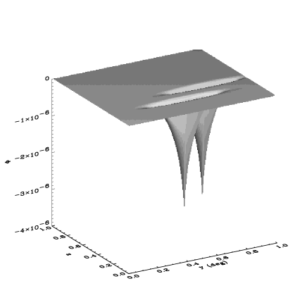
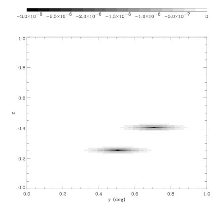
Figure 4: Example of gravitational potential. Here we simulate the gravitational potential for two NFW clusters at ${\mathbf{r}}=(0.5,0.5,0.25)$ and $(0.5,0.7,0.4)$; the upper panel is a 3-D representation of ($y,z,\Phi$) resulting from an $x$ slice at $x=0.5^{\circ}$; the lower panel displays the $\Phi$ values for ($y,z$) in greyscale.

We construct a 3-dimensional grid, typically with a total of $100^{3}$ points. This represents the redshift cone in which we will attempt to reconstruct the gravitational potential, i.e. the $x$ and $y$ directions represent an angular range on the sky, while the $z$ direction represents a radial distance. Typically we will use this to model angular scales in $x$ and $y$ of $1^{\circ}$ while probing in the $z$ direction down to an effective redshift of 1. We will therefore quote coordinates in $\mbox{\boldmath$r$}=(x,y,z)$ ranging from 0 to 1. This does not imply that the $z$ coordinate represents redshift, however; throughout this paper, $z$ represents a comoving distance measure.

This choice of coordinates significantly simplifies our analysis: in a flat universe, the comoving transverse separation of unperturbed light ray paths converging at an observer is proportional to the comoving radial distance along the light path (see e.g. Bartelmann & Schneider 2000, Section 6.1). Thus unperturbed rays will simply move along our $z$ coordinate with fixed $(x,y)$. Also, in order to lay down e.g. a constant 3-dimensional comoving number density of objects, we simply allocate a constant number density in our coordinates; no correction is necessary for a varying physical number density. Finally, the unitless transverse derivatives required in equation (2) are simply $\partial_{x}$ and $\partial_{y}$ in our coordinate system.

We fix in this grid the positions of lenses which we will wish to recover. We assign to each lens a mass and three perpendicular scale lengths for the size of its gravitational potential. In the following section we will be concerned with typical galaxy cluster lenses, in which case we assign masses in the range $0.5-5\times 10^{14}M_{\odot}$ and radii of $0.5-2$Mpc. We will position these clusters between $z=0.25$ and $z=0.5$ while probing lensed galaxies down to $z=1$, mimicking lensing studies of massive clusters (e.g. Tyson et al 1990, Kaiser & Squires 1993, Bonnet et al 1994, Squires et al 1996, Hoekstra et al 1998, Luppino & Kaiser 1997, Gray et al 2002).

Given these masses and scale lengths, we can calculate the gravitational potential over the entire 3-dimensional grid. We have used Navarro, Frenk & White (1996) profiles for the density,

$$\rho(\mbox{\boldmath$r$})=q/|\mbox{\boldmath$r$}-\mbox{\boldmath$r$}_{c}|(1+|\mbox{\boldmath$r$}-\mbox{\boldmath$r$}_{c}|)^{2},$$ (55)

where $q$ is a measure of the mass, and $\mbox{\boldmath$r$}_{c}$ are the coordinates of the centre of the mass profile. Using Gauss’s law and a further integration and renormalisation, we find the resulting gravitational potential for a mass concentration

$$\Phi(\mbox{\boldmath$r$})=-\frac{q_{1}r_{s}}{|\mbox{\boldmath$r$}|}\log\left(1+\frac{|\mbox{\boldmath$r$}-\mbox{\boldmath$r$}_{c}|}{r_{s}}\right),$$ (56)

with $q_{1}$ as a measure of mass and $r_{s}$ the NFW scale parameter. The total gravitational potential in the simulated volume of space is taken to be the sum of the individual lens contributions.

Figure 4 shows an example of our constructed gravitational potential, for two NFW profile clusters, placed at $z=0.25$ and $z=0.4$; the view is of a 1 grid-unit slice at $x=0.5^{\circ}$. The apparent distortion of the clusters is due to the scales chosen; we are examining a large distance scale radially ($\sim 3000$Mpc), with much smaller distance scales transversely ($\sim 10$Mpc). We will wish to reconstruct this gravitational potential for all $(x,y,z)$ from shear information only.

The masses of the clusters in this example were chosen to mimic the shear properties of clusters in Gray et al (2002), with mass $m=8\times 10^{13}M_{\odot}$ within a radius of 2 arcmin. Note that in order to calculate $\phi$ and $\Phi$ we convert the $x,y$ coordinates from degrees to radians, leading to the same $\phi$ and $\Phi$ normalisations as in Section 3.

From the gravitational potential shown in Figure 4, we calculate the lensing potential $\phi$ given by equation (7). This is a necessary step towards calculating the shear, which is all we will use for potential reconstruction. For each point in $(x,y)$ we set $\phi(x,y,0)=0$ and then use the discrete version of equation (7),

$$\phi(x,y,z)=-2\sum_{w=1}^{z}\frac{z-w}{zw}\Phi(x,y,w)\Delta w,$$ (57)

where we must first use this equation to calculate $\phi(x,y,0.01)$ then $\phi(x,y,0.02)$, etc. In this fashion, we can calculate the lensing potential for all points on our 3-dimensional grid.

Figure 5 shows the lensing potential calculated as above for the example introduced in Figure 4. Note that the axes on this 3-D plot are $(y,z,\phi)$; we are observing how the lensing signal grows with depth. The figure shows the generic behaviour for all lensing; the lensing potential due to distortion from a massive object becomes stronger with increasing depth, but asymptotes to a finite value at large $z$.

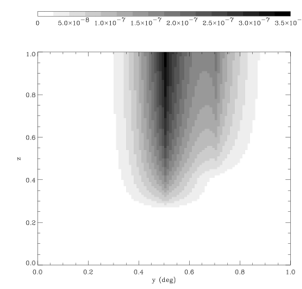
Figure 5: Lensing potential calculated for the gravitational potential of Figure 4. Note the increase in distortion expected with growing $z$. In the upper panel, the axes represent the $(y,z,\phi)$ coordinates; in the lower panel the $\phi$ values for ($y,z$) are shown in greyscale.

We are now in a position to calculate the 3-dimensional gravitational shear field arising from the gravitational potential. We calculate the shear components $\gamma_{1}$ and $\gamma_{2}$ from our 3-dimensional $\phi$ field by first approximating

$$\partial_{xx}\phi({\mathbf{x}}) \simeq [\phi(x+\Delta x,y,z)+\phi(x-\Delta x,y,z)$$ (58)

$$-2\phi(x,y,z)]/(\Delta x)^{2}.$$

An entirely similar approximation is made for $\partial_{yy}\phi({\mathbf{x}})$, while we approximate

$$\partial_{xy}\phi({\mathbf{x}}) \simeq \frac{1}{4}[\phi(x+\Delta x,y+\Delta x,z)+\phi(x-\Delta x,y-\Delta x,z)$$ (60)

$$-\phi(x-\Delta x,y+\Delta x,z)$$

$$-\phi(x+\Delta x,y-\Delta x,z)]/(\Delta x)^{2}.$$

Then, following from equation (2), we can write the shear components as

$$\gamma_{1}({\mathbf{x}})=-\frac{1}{2}(\partial_{xx}\phi({\mathbf{x}})-\partial_{yy}\phi({\mathbf{x}}))$$ (61)

$$\gamma_{2}({\mathbf{x}})=-\partial_{xy}\phi({\mathbf{x}})$$ (62)

From these equations we can calculate shear values for all points on our 3-dimensional grid. An example of a calculated shear field is shown in Figure 6, corresponding to the gravitational potential of Figure 4; this is an $(x,y)$ slice of the 3-D shear field at $z=0.75$. Note the clear signatures due to the two clusters. A slice further back in $z$ would have a similar $x,y$ pattern but a larger shear magnitude; a slice in $z$ in front of the clusters would have no shear signal.

Figure 6: Slice of the 3-D shear field corresponding to the gravitational potential of Figure 4. This is an $(x,y)$ slice at $z=0.75$. The largest $\gamma$ value plotted is 0.27.

We have therefore calculated the gravitational shear which would exist for an object at any grid point; now we must place objects at some of these grid positions, with an appropriate distribution in space. We normalise the total number of objects to those expected in surveys down to the required depth; for a ground-based survey probing to a limiting redshift $z_{r}=1$, we expect a number density $n\simeq 30$ usable galaxies per square arcmin (e.g. Bacon et al 2002). Alternatively, we can project the number densities expected for deep, space-based surveys down to $z_{r}=1$ ($n\simeq 100$; see Massey et al 2002).

The selected total number density is used to find the probability of an object existing at a given grid point in the following fashion. We treat each $(x,y)$ sheet as a slice of a comoving pyramid (not a box), in order to take into account the fact that the survey has an angular extent. In some of the simulations we will assume that the 3-dimensional number density is constant, while in others we will adopt $dN/dz\propto z^{2}\exp(-az^{2})$; the distribution will be stated in each case.

In the case of varying $N(z)$, the number of galaxies $N$ expected per grid point can be found using

$$N(x,y,z)=\frac{dN}{dz}\frac{\Delta z}{(\theta)^{2}}$$ (63)

where $\theta$ is the transverse survey length (usually $1^{\circ}$ in our simulations), $\Delta z$ is the radial grid increment, and $N_{tot}=n\Omega$, where $\Omega$ is the solid angle extent of the survey. For each $z$, we then generate $N(z)\theta^{2}$ random coordinates in $x$ and $y$, and increment the number of objects at the nearest grid point for each coordinate pair.

For each object, a random Gaussian-distributed shear value is chosen to simulate the effect of intrinsic ellipticity, and is added in quadrature to the gravitational shear value. For typical ground-based surveys the scatter in shear estimators due to the intrinsic ellipticity can be well modelled by Gaussians in $\gamma_{1}$ and $\gamma_{2}$ with standard deviation 0.3 in each component (e.g. Bacon et al 2002). For space-based survey simulations, we use the smaller standard deviation of 0.2 in each shear component (see e.g. Rhodes et al 2001).

We now have a set of galaxies sampling the 3-D shear field at a finite set of points in space, with an additional shot noise contribution from their intrinsic shapes. We must now attempt to estimate the underlying purely gravitational 3-D shear field, and from that to calculate the 3-D lensing potential $\phi$ from equation (9), and the corresponding 3-D gravitational potential $\Phi$ from equation (8).

4.2 Reconstructing the Potential

We can overcome the shot noise from galaxy ellipticities by a combination of binning many galaxies’ shears in a cell, and smoothing the shear field. In the specific examples given below, we find it convenient to initially rebin our galaxy grid to pixels with 3 arcmin diameter in the transverse direction and $\Delta z=0.05$ in the radial direction; further smoothing can be carried out as necessary later. We calculate the averaged shear field for the rebinned grid; this averaged shear will then be the basis of our potential reconstruction.

We can conveniently find the $\phi$ field corresponding to this $\gamma$ field using Fourier tranforms of these two fields. Following Kaiser and Squires (1993), we find from equation (9) an optimal estimate of the lensing potential,

$$\phi({\mathbf{k}})=\frac{2(k_{x}^{2}-k_{y}^{2})\gamma_{1}({\mathbf{k}})+4k_{x}k_{y}\gamma_{2}({\mathbf{k}})}{k_{x}^{2}+k_{y}^{2}},$$ (64)

where $\phi({\mathbf{k}})$ etc are Fourier transformed quantities. This equation is valid if the transverse differential operators of equation (9) are dimensionless; this is satisfied by our model, where the $x$ and $y$ directions represent angles rather than physical distances.

In this fashion we calculate $\phi({\mathbf{k}})$ using Fast Fourier Transforms, and hence find $\phi$. Since noisy low-$k$ modes can introduce rather large variability in $\phi$ with $z$ (see Section 2), we further add a constant at the edge of our (real-space) field to ensure that the mean of $\phi$ around the edge of the field is zero (this is equivalent to equation (12) above; see Section 3.1.2 and 3.2 for a discussion of the level of error this causes). We can then smooth the $\phi$ field in the $z$ direction to reduce the noise amplitude, convolving the $\phi$ field with a radial Gaussian. We can choose the width of this kernel in each circumstance as a compromise between reducing noise and retaining spatial resolution.

We then calculate the gravitational potential $\Phi$ using equation (8). As in equations (58) and (60), we use local differences in $\phi$ in the $z$ direction to approximate the derivatives. If necessary, we can smooth or filter $\Phi$ itself to further reduce noise levels.

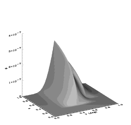
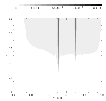
Figure 7: Top and middle panel: reconstructed lensing potential using the full shear field of Figure 6, in a $100^{3}$ grid. This is a $(y,z)$ plane at $x=0.5^{\circ}$. Bottom panel: difference between input and recovered lensing potential fields.

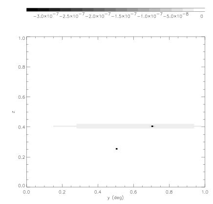
Figure 8: Top panel: reconstructed gravitational potential using the full shear field of Figure 6, in a $100^{3}$ grid. This is a $(y,z)$ plane at $x=0.5^{\circ}$. Bottom panel: difference between input and recovered gravitational potential fields.

5 Simulation Results

We have described above our means of simulating mass distributions and corresponding shears, followed by our method for reconstructing the lensing potential and gravitational potential given a finite number of noisy estimators of the shear. Here we describe our findings for this reconstruction.

5.1 Perfect reconstruction

First we examine the accuracy of our method when the shear field is perfectly known everywhere. Figure 7 shows the reconstruction of the lensing potential when we simply input into our reconstruction the full shear field shown in Figure 6; we do not smooth the shear field in this case. We regain the lensing potential successfully; this is quantified in Figure 7c, where we show the difference between the reconstructed and original $\phi$ fields, for a slice through the reconstruction. This error introduced by our numerical implementation is $<3$% of the lensing signal everywhere behind the clusters within 0.15 degrees of the cluster centres. The one exception is the core pixel line behind each cluster, where the error is 6.6% and 9.7% of the lensing potential for the left and right cluster respectively. This is expected, due to the cusp within this pixel, which the binned shear cannot accurately follow. We see that our procedure for reconstructing the lensing potential is very successful in the absence of noise.

We proceed to use our reconstructed lensing potential to find the 3-D gravitational potential, still using the full shear field (i.e. still without sampling by a finite number of objects, or adding shot noise due to galaxy ellipticities). Our result is shown in Figure 8, which displays the reconstructed $\Phi$ and the difference between input and reconstructed fields. Again it can be seen that, with perfect knowledge of the shear field, a good reconstruction is achieved with our method. For the cluster at $z=0.25$, the error is $<0.4$% of the signal within a radius of 0.2 degrees of the cluster, except for the core pixel where the error is 11.5%. For the cluster at $z=0.5$, the error is $<5\%$ of the signal within a radius of 0.1 degrees of the cluster, except for the core pixel where the error is 17.6%. This is again due to the cusp at the cluster centre, which cannot be followed well by our averaged shear field. Nevertheless, it is clear that our method is successful in reconstructing cluster gravitational potentials in the absence of noise.

5.2 Reconstruction with noise

Having demonstrated that the inversions of the shear field to obtain lensing and gravitational potentials are viable in the absence of noise, we now wish to add the two primary sources of noise present in lensing experiments: Poisson noise due to only sampling the field at a finite set of galaxy positions, and additional noise due to galaxies’ non-zero ellipticities. We use appropriate number densities for plausible ground-based experiments (30 per sq arcmin) and space-based experiments (100 per sq arcmin), and use equation (63) to place an appropriate number of objects at each redshift slice. We continue to use the gravitational potential of Figure 4.

We incorporate the effect of the intrinsic ellipticities of the galaxies as described in Section 4 (i.e. adding a Gaussian-distributed random shear value to the gravitational shear, with a standard deviation of 0.2 per shear component for space-based applications and 0.3 for ground-based applications).

Given this noisy shear field, we carry out our reconstruction as described in Section 4, with a Gaussian smoothing of the $\phi$ field in the $z$ direction with a $1\sigma$ width of 0.1 in redshift (not applied for calculating Wiener-filtered $\Phi$).

We will now discuss the reconstructions obtained for ground-based and space-based data. In the discussion below, we will often describe measurement significance in terms of $\nu({\mathbf{x}})=I({\mathbf{x}})/\sigma({\mathbf{x}})$, with $I({\mathbf{x}})$ the amplitude of the lensing potential or gravitational potential at a particular point ${\mathbf{x}}$, and $\sigma({\mathbf{x}})$ the noise level in the vicinity of this point.

5.2.1 Lensing Potential for Space-based Experiment

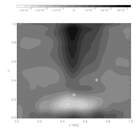
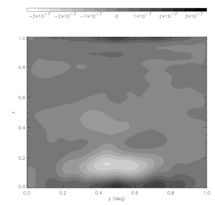
Figure 9: Top panel: reconstructed lensing potential $\Delta\phi$ using finite number of galaxies with realistic ellipticities; $n=100$ per sq arcmin, $\gamma_{\rm rms}=0.2$ per shear component, as expected for a notional space-based survey. Crosses show the positions of the cluster centres. Bottom panel: difference between input and recovered lensing potential fields.

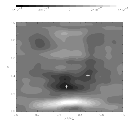
Figure 10: Reconstructed gravitational potential for our space-based experiment, using galaxy properties as in Figure 9, after Wiener filtering. Note the detections of clusters at $(y,z)=(0.5,0.2)$ and $(0.7,0.4)$ with $\nu=4.2$ and 2.1 respectively (crosses show trough minima).

The resulting lensing potential reconstruction for our space-based experiment is shown in the top panel of Figure 9. (In this and later figures, we plot the results for our $20^{3}$ grid, but display a resampled grid calculated by padding the Fourier transform of the grid with high-$k$ modes set to zero.) We find that we obtain a reasonable reconstruction of the lensing potential, with $\nu\simeq 6.9$ per pixel in the background ($z>0.75$) for the nearer cluster, with $\nu\simeq 4.2$ for the $z=0.4$ cluster, within 0.1 deg radius of the cluster centres. We could increase this signal by rebinning or smoothing, at the cost of reducing spatial resolution. We could also find an overall signal-to-noise for each cluster by finding a means of averaging all of the lensing signal arising behind a cluster; we will discuss this in Section 7. Note the large noise peaks in the foreground ($z<0.2$) of the reconstruction, due to the small number of objects available in this volume.

The lower panel of Figure 9 shows the difference between the input and recovered lensing potential. Pleasingly, we observe no evidence of residuals associated with misconstruction of the lensing potential. The noise levels are as expected from equation (20), as discussed in Section 6 below.

5.2.2 Gravitational Potential for Space-based Experiment

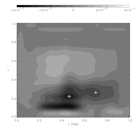
Figure 11: Reconstructed gravitational potential for a notional ground-based survey, after Wiener filtering; $n=30$ per sq arcmin, $\gamma_{\rm rms}=0.3$ per shear component. The clusters are measured with $\nu=1.9$ and $\nu=1.4$.

On the other hand, we find that the full 3-D reconstruction of the gravitational potential for typical cluster masses is difficult even from space unless we include filtering (see Section 6.1). For example, a measurement of the gravitational potential for a set of 25 clusters with mass $m=8\times 10^{13}$ within 2 arcmin added together at $z=0.25$, having smoothed $\phi$ in the radial direction with a top hat with $\Delta z=0.25$, produces a gravitational potential amplitude for the central pixel of the cluster which is only 3.1 times larger than the rms noise. However, the noise amplitude for larger $z$ grows rapidly (c.f. Section 6.1), making 3-D measurement of a resolved cluster potential difficult without filtering.

In order to improve on this, we can use the Wiener filtering described in Section 3. We create a vector $\mathbf{P}$ containing our measured gravitational potential along each line in the $z$ direction, and measure the covariance of the $\Phi$ noise along this line of sight from 100 zero-$\phi$ reconstructions of $\Phi$, recording this in a matrix $\mathbf{N}$. We set the signal covariance matrix ${\mathbf{S}}=(3\times 10^{-7})^{2}\mathbf{1}$ where $\mathbf{1}$ is the unit matrix, in order to select for a signal expected for a small cluster mass (cf Figure 8). We then apply equation (40) to our gravitational potential vector for each line of sight.

Figure 10 shows the gravitational potential measurements for our notional space-based survey after Wiener filtering (this is again a reconstruction for the single field shown in Figure 8; after Wiener filtering we no longer need to stack many fields to obtain a signal). We measure the $z=0.25$ cluster with $\nu=4.2$ at the peak (trough) pixel of its gravitational potential well, with $\nu=2.1$ at the gravitational potential trough of the $z=0.4$ cluster. We also find a substantial noise peak in the foreground at $z=0.1$. While the recovery of the cluster gravitational potentials therefore constitutes a challenging measurement, we are indeed able to reconstruct useful information in the gravitational potential field itself. (The detection significance of these clusters is much higher than the measurement $\nu$ at a given point in the cluster; see Section 7 for an approach to the detection significance.) Note the reduced absolute amplitude of the gravitational potential in Figure 8; this is due to the scaling in equation (40).

5.2.3 Gravitational Potential for Ground-based Experiment

From the ground, we find that we can again reconstruct the lensing potential, with $\nu\simeq 2.3$ for $0.75<z<1.0$ given a cell size of 0.05 in $z$. As before, we could improve the signal-to-noise by reducing our spatial resolution. However, reconstruction of the gravitational potential itself (with Wiener filtering) is more challenging than from space: Figure 11 demonstrates that we recover the $z=0.25$ cluster with $\nu=1.9$ at its centre pixel, but have a less significant measurement of the second cluster amplitude with $\nu=1.4$ at its centre. The second cluster has the expected position in $(x,y)$, but is offset to $z=0.3$; this degree of offset, $\Delta z=0.1$, is found to be typical for ground-based attempts at measuring the 3D gravitational potential, due to the high $\Phi$ noise level making Wiener filtering somewhat inaccurate in the $z$ direction. As with our space-based experiment, we also find a substantial noise peak in the foreground at $z=0.1$.

6 Prospects for Mapping

The results above are encouraging for the mapping of the 3-D lensing fields. This includes the gravitational potential; we can use Wiener filtering to detect individual mass concentrations, or can stack the noisy potential field from many clusters in order to obtain information on the typical gravitational profile of mass concentrations. Here we will examine the prospects for mapping with the various 3-D fields we have discussed so far, paying close attention to the noise contributions to each field.

Figure 12: Noise variance for 1 pixel (0.05 deg, 0.05 in $z$) as a function of $z$ for the 3-D convergence field $\kappa$. The thin solid line represents the measured noise level for our fiducial space-based experiment, while the dashed line represents measured noise from our ground-based experiment. The dotted line shows the expected signal from a cluster at $z=0.2$. The thick solid line shows the noise expected from theory for the ground-based survey, from equation (15); we see that there is close agreement between simulations and theory.

Figure 13: Noise variance for 1 pixel (0.05 deg, 0.05 in $z$) as a function of $z$ for the lensing potential in a 1 deg² square survey. The solid line represents the measured noise level for our fiducial space-based experiment, while the dashed line represents measured noise from our ground-based experiment. The dash-dotted line shows the effect of redistributing the galaxies according to equation (63) for our space-based experiment. The dotted line shows the expected signal from a cluster at $z=0.2$. The thick solid line shows the noise expected from theory for the ground-based survey, from equation (20); we again find good agreement between simulations and theory.

Figure 14: Noise variance for 1 pixel (0.05 deg, 0.05 in $z$) as a function of $z$ for the gravitational potential. The solid line represents measured noise level for our fiducial space-based experiment, while the dashed line represents measured noise from our ground-based experiment. Top: standard gravitational potential reconstruction. The dotted line shows the expected signal from a cluster at $z=0.2$. The thick solid line shows the noise expected from theory for the space-based survey, from equation (22); we again find good agreement between theory and simulation. Bottom: Wiener filtered reconstruction. The spikes show the measured Wiener-filtered amplitude of a $10^{14}M_{\odot}$ cluster at $z=0.2$ and $z=0.4$ for ground-based (dotted) and space-based (solid) noise levels.

6.1 Noise amplitudes

In order to demonstrate the feasibility of our reconstructions, we examine the noise from convergence, lensing potential and gravitational potential maps measured in our simulations as a function of $z$. Figure 12 shows the rms noise amplitude for $\kappa$ as a function of redshift; Figure 13 shows the corresponding uncertainty in $\phi$, while Figure 14 shows the uncertainty in $\Phi$. In each case, we show the measured noise amplitude for space-based and ground-based experiments, measured as a function of $z$, along with the expected potential amplitude from a $m=10^{14}M_{\odot}$ cluster. Here we have used the averaging scales described above, i.e. we have calculated the noisy $\kappa$ and $\phi$ fields on a grid with total width 1 degree, with grid spacing of 0.05 degree and 0.05 $c/H_{0}$ in $z$. It is simple to derive noise amplitudes for other survey configurations from equations (19) and (22).

We see from from the theoretical curves on Figure 12 that the noise amplitude measured for the convergence field is in good agreement with that calculated in Section 2. Similarly, we see that the measured noise amplitude for $\phi$ in Figure 13 agrees well with the predicted theoretical curve. Lastly, we see in Figure 14 that the uncertainty in gravitational potential is in agreement with our theoretical model.

Note that, for the convergence and lensing potential, the noise amplitude is such that $\nu\simeq 6$ measurement of these fields from a typical $z=0.2$ cluster is possible in (0.05 degree, 0.05 in redshift) bins in a space-based experiment, if we examine the background potential at $z>0.5$ in the centre of the cluster. For a ground-based experiment, the signal-to-noise in these bins is $\simeq 3$. Thus as we saw above, it is possible to map the properties of clusters in terms of the lensing potential from space or ground. Note the effect in Figure 13 of redistributing the galaxy distribution according to equation (63); the amplitudes of the noise are comparable, with a slight decrease in noise at low redshift and a corresponding increase at high redshift for the galaxy distribution of equation (63).

On the other hand, the gravitational potential without Wiener filtering is only measured at $\nu=0.38$ in equivalent bins around $z=0.2$ for space-based experiments, and has a signal-to-noise of only $\simeq 0.12$ for ground-based measurements. Since the noise reduces as $\sqrt{N}$ where $N$ is the number of stacked fields, we would have to stack $\sim 40$ fields in order to resolve the gravitational potential at the $\nu=2.5$ level, for a space-based experiment without Wiener filtering. Increasing the size of bins is not an option in this case, as we will lose spatial resolution for examining the profile of the cluster.

However, Wiener filtering allows us to recover cluster masses successfully, as shown in the bottom panel of Figure 14. Here we see that, for a cluster mass of $10^{14}M_{\odot}$ at $z=0.25$, we obtain $\nu=2.1$ measurements from the ground and $\nu=3.3$ measurements from space. Note the differing noise and signal levels expected after Wiener filtering for ground and space-based experiments; this is due to the differing weightings in equation (40) given different input noise levels.

6.2 Dependence on transverse and radial pixel sizes

Figure 15: Noise variance for the lensing potential at z=1 as a function of angular pixel size, for our space-based experiment, with a 1 deg² square survey.

Figure 16: Noise variance for the gravitational potential as a function of pixel size in the radial direction, for our space-based experiment (at z=0.4, 1 deg² survey, angular pixel diameter 3’). The dotted line is the expected dependence from equation (22).

The effect of increasing the angular pixel scale in a survey is of interest, as this might be thought to increase signal-to-noise. However, Figure 15 shows how an increase in pixel size for a fixed survey size reduces the lensing potential noise variance. We note that the effect is small until a pixel size $\sim 0.25\Theta_{survey}$ is used; at this point, the pixel size will usually be far too large to be of use to us, as we will typically be interested in spatially resolving objects with the lensing potential. The cause of the decrease in noise as pixel size increases is partially the ln $r$ force law involved in the analysis in Section 3.1.2, and partially the increased bin size leading to averaging out of the small-scale noise.

Figure 16 shows the effect of increasing the radial bin size for the gravitational potential reconstruction. We see a reduction of the noise level in agreement with equation (22), i.e. $\sigma(\Phi)\propto(\Delta z)^{-5/2}$. Thus if we are unconcerned with radial resolution, we can increase our signal-to-noise for gravitational potential by increasing $\Delta z$; however, we will often be attempting to locate a mass concentration in the radial direction, so this procedure should be used with caution.

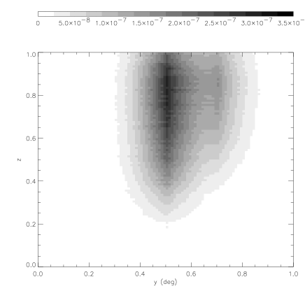
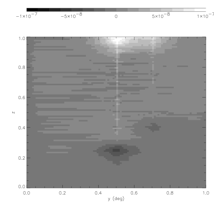
Figure 17: Top panel: reconstructed lensing potential using the full shear field of Figure 6, while including redshift uncertainty $\Delta z=0.1$. This is the usual $(y,z)$ plane at $x=0.5$. Bottom panel: difference between input and recovered lensing potential fields.

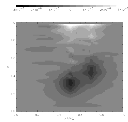
Figure 18: Reconstructed gravitational potential using the full shear field of Figure 6, including redshift uncertainty $\Delta z=0.1$.

6.3 Redshift Errors

In the above simulations, we have demonstrated that the Poisson noise of sampling from a finite set of galaxies, together with the noise due to galaxy ellipticities, represent serious sources of uncertainty for our reconstruction, which must be overcome by averaging the signal within sufficiently large pixels or filtering the signal. However, there remains the further source of error due to redshift measurement uncertainty, which we examine here with our simulations (see Sections 3.4 and 3.5 for analytical discussion).

We can examine redshift errors with our simulations by allowing an uncertainty in the redshift of each galaxy, in the following fashion. For each galaxy, a $z$ value is drawn uniformly within the $z$ slice in question; an uncertainty is introduced in this $z$ coordinate, by drawing from a Gaussian random variable with $1\sigma$ width $\Delta z=0.1$ (pessimistically, for photometric redshifts; cf Brown et al 2002 with $\Delta z=0.05$ in $0<z<0.8$). If the new $z$ coordinate (resulting from adding this random offset to the original $z$ position) is moved to a new shell, the galaxy (with its shear calculated for the slice which it intially belonged to) is moved to the neighbouring slice.

Figures 17 and 18 show the result of this process when the shear is fully known everywhere; note that even with this large redshift uncertainty, the change in the lensing potential reconstruction is small ($\simeq 10$% at redshifts near the cluster redshift, and less elsewhere). Note that this smearing effect leads to slightly higher lensing potentials in front of the cluster, and slightly slower rise in the potential behind the cluster. Thus, for lensing potential reconstructions, this effect will not dominate the noise. However, Figure 18 shows that the result of such an uncertainty will be a smearing of the cluster gravitational potential with smearing width $\simeq\Delta z$; understandably, we cannot reconstruct the potential with a resolution greater than our redshift resolution.

7 3-D Information from the Lensing Potential

Figure 19: 1 and 2$\sigma$ $\chi^{2}$ fit constraints on $z$ and $m$ for 1 cluster along a line of sight, $m=8\times 10^{13}M_{\odot}$, with noise appropriate for our space-based experiment. Here we are fitting the simulated 3-D $\phi$ field with the $\phi$ field from a 2-D NFW profile with parameters ($z,m$).

Figure 20: Best fit model for $\phi$ field along line of sight through centre of a cluster with $m=8\times 10^{14}M_{\odot}$, with noise appropriate for our space-based experiment.

It will be noted from our simulations that recovery of the gravitational potential is more difficult than an adequate reconstruction of the lensing potential. It is easy to see why this should be so; the gravitational potential requires double differentiation of the already noisy lensing potential field. Therefore we are interested in both the lensing and gravitational potentials; while the lensing potential is more easily accessible, and itself contains useful topological information about the mass field, the gravitational potential is the more fundamental quantity.

A particular example of what is achievable by studying the $\phi$ field is the characterisation of the 3-D matter distribution on cluster scales. Treating a cluster as a mass delta function in the $z$ direction (c.f. Hu & Keeton 2002), it is clear from equation (7) that the expected lensing potential in a flat universe due to a cluster at radial position $r_{s}$ will be

$$\phi(z)=\left\{\begin{array}[]{ll}0&r\leq r_{s}\\ 2\rho dV\frac{r-r_{s}}{rr_{s}}&r>r_{s}\\ \end{array}\right.$$ (65)

where $\rho dV$ is the mass content of the source pixel.

We can use a superposition of such cluster contributions to fit a given $\phi$ field, and thus discover significant clusters behind clusters, for example (c.f. Hu & Keeton 2002). We can also directly measure constraints on mass and position of clusters without using the redshift of the cluster members themselves (e.g. Wittman et al 2001, 2002).

7.1 Single cluster $\chi^{2}$ fitting

In order to demonstrate these applications, we first simulate a cluster at $z=0.25$ with mass $8\times 10^{13}M_{\odot}$ within a 2 arcmin radius using the simulation recipe described in Section 3, including realistic galaxy distribution and ellipticity (using our space-based parameters, $n=100$, $\sigma_{\gamma}=0.2$ per component). After measuring the resulting $\phi$ field as in Section 4, we applied a $\chi^{2}$ fitting procedure for the mass $m$ and position $z$ of the cluster. This was achieved by setting up a 2-D NFW profile at radial position $z$, normalised to mass $m$; the expected 3-D $\phi$-field for this profile was calculated according to equation (65). $\chi^{2}$ for the data with respect to this profile was calculated for an array of $m$ and $z$ values, with step size $2.5\times 10^{11}M_{\odot}$ in $m$ and 0.005 in $z$. Note that the $x,y$ position and radius of our NFW test profile were fixed to the actual position and radius of the cluster in this experiment; in a practical scenario one would apply a $\chi^{2}$ fit for these parameters as well, or infer them from the galaxy positions of cluster members.

Figure 19 shows the resulting constraints on mass and radial position; we find a highly significant detection of the cluster at the $\Delta\chi^{2}=186$ level, thus we can certainly use this 3-D approach to detect at least one cluster along the line of sight. We obtain accurate measurements of the mass ($m=(8.07\pm 0.83)\times 10^{13}M_{\odot}$ within 2’ radius) and position $(z=0.24\pm 0.016)$, which makes this approach promising for examining clusters in 3-D. Figure 20 demonstrates a best-fit $\phi$ field for this form of simulation, with mass multiplied by 10 for illustrative purposes.

Figure 21: 1 and 2$\sigma$ $\chi^{2}$ fit constraints on $z_{1}$ and $z_{2}$ for 2 clusters along line of sight, with noise appropriate for our space-based experiment, having marginalised over the masses of the two clusters.

Figure 22: 1 and 2$\sigma$ $\chi^{2}$ fit constraints on $m_{1}$ and $m_{2}$ for 2 clusters along line of sight, with noise appropriate for our space-based experiment, having marginalised over the positions of the two clusters.

Figure 23: 1, 2 and 3$\sigma$ $\chi^{2}$ fit constraints on $m_{1}$ and $m_{2}$ for 2 clusters along line of sight, with noise appropriate for our space-based experiment, after including redshift measurements of cluster positions.

Figure 24: Best fit model for $\phi$ field along line of sight through centre of 2 clusters, $m=8\times 10^{14}M_{\odot}$, at $z=0.25$ and 0.5. The dotted line represents the $\phi$ field arising from the $z=0.25$ cluster alone.

7.2 $\chi^{2}$ fitting for two clusters along the line of sight

We can examine the possibility of detecting clusters behind clusters by simulating an $8\times 10^{13}M_{\odot}$ cluster (2 arcmin radius) at $z=0.6$ behind another $8\times 10^{13}M_{\odot}$ cluster at $z=0.25$, and applying a $\chi^{2}$ fit for two masses and positions using the method above.

Figures 21 and 22 show the constraints we obtain on mass and position of the two clusters from the simulation, having marginalised over the 4-dimensional $\chi^{2}$ distribution to find a subset of parameters. We see that, for this example, two configurations of clusters are possible: (a) two clusters very near each other in redshift; this is essentially the discovery of a 1-cluster solution. (b) One cluster at $z=0.25$ with another of similar mass at $z=0.6$; this is the solution corresponding to our input scenario. In this case, we obtain greater accuracy in measuring the mass for the nearer cluster. This can be understood from Figure 24 (displaying masses 10 times larger for illustrative purposes): much of the background $\phi$ amplitude is due to the first cluster, so the mass and position of this cluster is well-constrained; on the other hand, the second cluster’s $\phi$ contribution has less distance in which to rise, so this cluster’s mass and position estimates are more affected by the noise amplitude.

If this double solution were present when the fitting procedure was applied to real data, we could easily use our sample redshifts to confirm one scenario by looking for increased number-counts at the claimed cluster redshifts. By confirming the redshift of the cluster in this fashion, we can obtain better estimates of the mass, together with a more conclusive statement as to whether there are mass concentrations in the background. This is demonstrated in Figure 23. Here we have again simulated a cluster behind a cluster; we have now allowed the clusters to have known redshifts in our $\chi^{2}$ fit. In this case we find that a two-cluster fit is substantially better than a one cluster fit (i.e. $m_{2}=0$) at the $2\sigma$ level. We find best values for the masses of the clusters to be $m_{1}=(8.46^{+0.31}_{-0.35})\times 10^{13}M_{\odot}$ and $m_{2}=(6.63^{+3.92}_{-3.79})\times 10^{13}M_{\odot}$ (c.f. input $m_{1,2}=8\times 10^{13}M_{\odot}$) within 2 arcmin radii. If we only constrain $z_{1}$, we find a best fit value for the background position of $z_{2}=0.6\pm 0.05$ (c.f. input $z=0.6$); thus if we have found a low-redshift cluster, we can check if there are significant clusters behind it.

We could increase the number of clusters in our $\chi^{2}$ fit, in order to seek for $>2$ clusters along the line of sight. However, in this case we will begin to fit the noise rather than real structures; this will be seen as too good a fit in our $\chi^{2}$ (i.e. $\Delta\chi^{2}\la\sqrt{2(x/\Delta x)(y/\Delta y)(z/\Delta z)}$). This restricts our ability to construct accurate 3-D maps using this method; however, we can at least map up to the first few significant mass concentration in the $z$ direction, and cosmological information could be gained by determining the statistical properties of the distance to the first or first few mass concentrations.

One can envisage, therefore, a procedure consisting of (a) initial detection of mass concentrations using the 3-D distortion field alone, followed by (b) improved mass and background structure estimates by assigning accurate redshifts from the visible matter associated with the detected foreground mass concentrations.

8 Conclusions

In this paper, we have developed and tested a practical method for 3-D reconstruction of the gravitational potential via weak lensing measurements, together with the more easily obtained lensing potential. This methodology is based on the reconstruction equations of Kaiser & Squires (1993) and Taylor (2002), by which these local 3-D potentials can be calculated given knowledge of the lensing shear field in 3-D. This can be obtained by using shear estimators for galaxies with known redshifts.

We have presented analytical forms for the shot-noise uncertainty in the convergence, lensing potential, gravitational potential and density field, noting that these fields become progressively more noisy for realistic survey sizes. We have also calculated the effects of only having finite sky-coverage for a survey and estimated the variance measured on such a survey, and the additional uncertainty in the reconstruction due to structure beyond the survey boundary. In particular we have found that the contribution to the reconstruction uncertainty in the differential lensing potential, $\Delta\phi$, is dominated by large-scale structures.

We have also shown that further sources of error, including photometric redshift errors, redshift-space distortions, and multiple scatterings of light rays, will not be dominant in our reconstruction process.

In order to simulate the measurement of a 3-D gravitational field, we have calculated the expected lensing potential due to a given mass field upon a 3-D grid. From this we have calculated the shear expected upon a galaxy image for a galaxy positioned anywhere in the 3-D grid. We have produced a catalogue of galaxies positioned in accordance with a realistic redshift distribution and given each an appropriate shear plus a random intrinsic ellipticity; this final galaxy shear catalogue was the information given to our reconstruction software.

We have made reconstructions of the lensing and gravitational fields, by smoothing the noisy shear data, calculating the lensing potential according to Kaiser & Squires (1993) and using Taylor’s equation (8) to find the gravitational potential.

We have found that the method works well in reconstructing the full lensing and gravitational potentials in the absence of noise. However, the addition of Poisson sampling of the field at a finite set of galaxy positions, together with the noise due to the intrinsic ellipticity of objects, produces significant sources of error. We find that we obtain lensing potential maps with $\nu\simeq 6$ in [3’, 3’, 0.05] bins in angle and redshift for a cluster of mass $8\times 10^{13}M_{\odot}$. Unfortunately, corresponding gravitational potential maps have only $\nu\simeq 0.5$ in pixels of this size. However, applying Wiener filtering to this gravitational potential, we can obtain $\nu\simeq 3$ measurements of gravitational potential of clusters of mass $8\times 10^{13}M_{\odot}$.

This provides excellent prospects for obtaining cosmologically significant information directly from the measured gravitational potential field. For surveys with a redshift limit $z=1$, mass concentrations $\ga 10^{14}M_{\odot}$ can be directly mapped between $0.1\la z\la 0.5$, while statistical mapping can be used to examine the gravitational potential fluctuations on smaller mass scales.

We have examined the effect of redshift uncertainties upon our simulations, and find that these contribute a much smaller error than the dominant intrinsic ellipticity noise term.

Finally we have emphasised that, even on scales where a gravitational potential measurement is uncertain, the 3-D measurement of the $\phi$ field is valuable, and can give us useful information about the statistics and topology of the mass field. In particular, we can obtain accurate measurements of the mass and position of clusters along the line of sight, and significantly detect the presence of clusters behind clusters.

The methodology described here for engaging in 3-D gravitational mapping has numerous applications. We can obtain direct measurements of mass distributions in 3-D, which can act as an important cosmological probe via the mass function or cluster number counts. We can directly measure cross correlation functions between mass and light in 3 dimensions. Also, for possible ’dark’ mass concentrations (e.g. Erben et al 2000), this 3-D mapping procedure allows us to measure both mass and radial position for such objects, which is quite impossible via conventional redshift methods.

9 Appendix: Calculating uncertainties on the 3D fields

Here we describe the details of our analysis for calculating uncertainties on the lensing and gravitational potentials.

9.1 The lensing potential field

In Section 3.1.2 we state the covariance of the 3-D lensing potential,

$$\langle\phi(\mbox{\boldmath$r$})\phi(\mbox{\boldmath$r$}^{\prime})\rangle_{SN}=4\partial^{-2}\partial^{\prime-2}\langle\kappa(\mbox{\boldmath$r$})\kappa(\mbox{\boldmath$r$}^{\prime})\rangle_{SN}.$$ (66)

We can calculate this covariance over the observed area, assuming a flat sky, obtaining

$$\langle\phi(\mbox{\boldmath$r$})\phi(\mbox{\boldmath$r$}^{\prime})\rangle_{SN}=$$ (67)

$$\frac{\gamma_{\rm rms}^{2}}{\pi^{2}n(r)r^{2}}\int_{A}d^{2}\theta^{\prime\prime}\ln|\mbox{\boldmath$\theta$}-\mbox{\boldmath$\theta$}^{\prime\prime}|\ln|\mbox{\boldmath$\theta$}^{\prime}-\mbox{\boldmath$\theta$}^{\prime\prime}|\delta_{D}(r-r^{\prime})$$

where the integral is taken over the survey area, $A$. The discrete case is an obvious change to a summation over bins.

Transforming to the differential potential field,

$$\Delta\phi=\phi-\overline{\phi},$$ (68)

where $\overline{\phi}$ is the mean field estimated from a finite survey of area $A$,

$$\overline{\phi}=\frac{1}{A}\int_{A}\!d^{2}\!\theta\,\phi(\mbox{\boldmath$\theta$}),$$ (69)

we find the covariance $\langle\Delta\phi(\mbox{\boldmath$r$})\Delta\phi(\mbox{\boldmath$r$}^{\prime})\rangle_{SN}$ is equivalent to equation (67) after transforming the kernel

$$\ln|\mbox{\boldmath$\theta$}-\mbox{\boldmath$\theta$}^{\prime}|\rightarrow\ln|\mbox{\boldmath$\theta$}-\mbox{\boldmath$\theta$}^{\prime}|-\frac{1}{A}\int_{A}\!d^{2}\!\theta\,\ln|\mbox{\boldmath$\theta$}-\mbox{\boldmath$\theta$}^{\prime}|.$$ (70)

In the simple case of a circular survey with radius $R$ we find

$$\frac{1}{A}\int_{A}\!d^{2}\!\theta^{\prime}\,\ln|\mbox{\boldmath$\theta$}-\mbox{\boldmath$\theta$}^{\prime}|=\frac{1}{2}[(\theta/R)^{2}-1+\ln R^{2}].$$ (71)

Note here we have assumed infinite resolution for the survey, or infinitely small pixels.

The uncertainty in the 3-D lensing potential difference is then given by

$$\langle\Delta\phi^{2}(\mbox{\boldmath$r$})\rangle_{SN}=\frac{\gamma_{\rm rms}^{2}}{\pi^{2}n(r)}\frac{\Theta^{2}(\mbox{\boldmath$\theta$})}{r^{2}}\delta_{D}(r-r^{\prime}),$$ (72)

where

$$\Theta^{2}(\mbox{\boldmath$\theta$})=\int_{A}\!d^{2}\!\theta^{\prime}\,\left[\ln|\mbox{\boldmath$\theta$}-\mbox{\boldmath$\theta$}^{\prime}|-\frac{1}{A}\int_{A}\!d^{2}\!\theta\,\ln|\mbox{\boldmath$\theta$}-\mbox{\boldmath$\theta$}^{\prime}|\right]^{2},$$ (73)

which in general has to be evaluated numerically. In the special case of $\mbox{\boldmath$\theta$}=0$ and a circular aperture with angular radius $\theta$, this can be evaluated analytically, giving

$$\langle\Delta\phi^{2}(\mbox{\boldmath$\theta$}=0)\rangle_{SN}=\frac{5}{24\pi}\frac{\gamma^{2}_{\rm rms}}{n(r)}\frac{\theta^{2}}{r^{2}}\delta_{D}(r-r^{\prime}),$$ (74)

where we have taken into account the conical geometry of the survey. This is the result discussed in Section 3.1.2.

9.2 The Newtonian potential field

In order to calculate the uncertainty on the 3-D Newtonian potential, we must smooth the field; this is because we require a double differentiation of the lensing potential, but only sample this field at discrete points where there are galaxies. If we smooth in the radial direction with an arbitrary smoothing kernel, $w(r)$, we find the resulting covariance matrix of the Newtonian potential for a constant galaxy number density, $n$, in the distant observer approximation, is

$$\langle\Phi(\mbox{\boldmath$r$})\Phi(\mbox{\boldmath$r$}^{\prime})\rangle_{SN}=\frac{\gamma^{2}_{\rm rms}}{4\pi^{2}n}\frac{\Theta^{2}(\mbox{\boldmath$\theta$},\mbox{\boldmath$\theta$}^{\prime})}{L^{3}(r,r^{\prime})},$$ (75)

where

$$\frac{1}{L^{3}(r,r^{\prime})}=\frac{r^{2}r^{\prime 2}}{R^{2}}\int\!dy\,w^{\prime\prime}(r,y)\,w^{\prime\prime}(r^{\prime},y)$$ (76)

has units of inverse volume. Dashes on the window function denote derivatives with respect to distance. If the number density of sources is not a constant, these formulae must be altered by the substitution

$$\frac{1}{nL^{3}(r,r^{\prime})}\rightarrow\frac{r^{2}r^{\prime 2}}{R^{2}}\int\!dy\,w^{\prime\prime}(r,y)w^{\prime\prime}(r^{\prime},y)/n(y).$$ (77)

Again we can evaluate these expressions for the variance in a bin when $r^{\prime}=r$ and assuming a Gaussian weighting function, $w(r)=[\sqrt{2\pi}r_{||}]^{-1}\exp(-r^{2}/2r_{||}^{2})$, with smoothing radius $r_{||}$. In this case to leading order, when $r\gg r_{||}$, and taking into account the conical geometry of the survey, the uncertainty on the Newtonian potential conveniently reduces to

$$\langle\Phi^{2}(r)\rangle_{SN}=\frac{5}{64\pi\sqrt{2\pi}}\frac{\gamma^{2}_{\rm rms}}{r_{||}^{3}n}\left(\frac{r}{r_{||}}\right)^{4}\left(\frac{r_{||}}{R}\right)^{2}\theta^{2}.$$ (78)

This is the result discussed in Section 3.1.3.

References

- [1] Bacon D., Massey R., Refregier A., Ellis R.S., 2002, submitted to MNRAS, astro-ph 0203134.
- [2] Bartelmann M., Schneider P., 2001, Phys. Rep., 340, 291.
- [3] Bernardeau F., van Waerbeke L., Mellier Y., 1997, A&A, 322, 1.
- [4] Bernstein G. M., Jarvis M., 2002, AJ, 123, 583.
- [5] Bonnet H., Mellier Y., Fort B., 1994, ApJL, 427, 83.
- [6] Broadhurst T., Taylor A.N., Peacock J., 1995, ApJ, 438, 49.
- [7] Brown M. L., Taylor A. N., Bacon D. J., Gray M. E., Dye S., Meisenheimer K., Wolf C., 2002, submitted to MNRAS, astro-ph 0210213.
- [8] Erben T., van Waerbeke L., Mellier Y., Schneider P., Cuillandre J.-C., Castander F. J., Dantel-Fort M., 2000, A&A, 355, 23.
- [9] Gray M. E., Taylor A. N., Meisenheimer K., Dye S., Wolf C., Thommes E., 2002, ApJ, 568, 141.
- [10] Heymans C., Heavens A., 2002, accepted by MNRAS, astro-ph 0208220.
- [11] Hoekstra H., Franx M., Kuijken K., Squires G., ApJ, 504, 636.
- [12] Hoekstra H., Yee H., Gladders M., Barrientos L. F., Hall P., Infante L., 2002, ApJ, 575, 55.
- [13] Hu W., 1999, ApJL, 522, 21.
- [14] Hu W., Keeton C. R., 2002, submitted to PRD, astro-ph 0205412.
- [15] Hu W., 2002, astro-ph 0208093.
- [16] Huterer D., 2002, PhysRevD, 65.
- [17] Jain B., Seljak U., 1997, ApJ, 484, 560.
- [18] Kaiser N., Squires G., 1993, ApJ, 404, 441.
- [19] Kaiser N., Squires G., Broadhurst T., 1995, ApJ, 449, 460.
- [20] Kaiser N., 1998, ApJ, 498, 26.
- [21] King L., Schneider P., 2002a, accepted by A&A, astro-ph 0208256.
- [22] King L., Schneider P., 2002b, A&A in press, astro-ph 0209474.
- [23] Luppino G. A., Kaiser N., 1997, ApJ, 475, 20.
- [24] Massey R. et al, 2002, in preparation.
- [25] Peebles P. J. E., Large-scale structure of the universe, 1980.
- [26] Refregier A. R., Bacon D. J., 2002, MNRAS in press, astro-ph 0105179.
- [27] Refregier A., Rhodes J., Groth E. J., 2002, ApJ, 572, 131.
- [28] Rhodes J., Refregier A., Groth E. J., 2001, ApJ, 552, 85.
- [29] Rhodes J., Refregier A., Groth E. J., 2000, ApJ, 536, 79.
- [30] Seljak U., 1998, ApJ, 506, 64.
- [31] Squires G., Kaiser N., Fahlman G., Babul A., Woods D., 1996, ApJ, 469, 73.
- [32] Taylor A.N., Dye S., Broadhurst T. J., Benitez N., van Kampen E., 1998, ApJ, 501, 539.
- [33] Taylor A. N., 2002, submitted to Phys Rev Lett, astro-ph 0111605.
- [34] Tyson J.A., Valdes F., Wenk R.A., 1990, ApJLett, 349, L1
- [35] van Waerbeke L., Mellier Y., Radovich M., Bertin E., Dantel-Fort M., McCracken H. J., Le Fevre O., Foucaud S., Cuillandre J.-C., Erben T., Jain B., Schneider P., Bernardeau F., Fort B., 2001, A&A, 374, 757.
- [36] Wittman D., Tyson J. A., Margoniner V. E., Cohen J. G., Dell’Antonio I. P., 2001, ApJ, 557, 89.
- [37] Wittman D., Margoniner V. E., Tyson J. A., 2002, submitted to ApJL, astro-ph 0210120.