Ultradeep Near-Infrared ISAAC Observations of the
Hubble Deep Field South:
Observations, Reduction, Multicolor Catalog, and Photometric Redshifts

Abstract

We present deep near-infrared (NIR) $J_{s}$, $H$, and $K_{s}$-band ISAAC imaging of the WFPC2 field of the Hubble Deep Field South (HDF-S). The $2.5\arcmin\times 2.5\arcmin$ high Galactic latitude field was observed with the VLT under the best seeing conditions with integration times amounting to 33.6 hours in $J_{s}$, 32.3 hours in $H$, and 35.6 hours in $K_{s}$. We reach total AB magnitudes for point sources of 26.8, 26.2, and 26.2 respectively ($3\sigma$), which make it the deepest ground-based NIR observations to date, and the deepest $K_{s}$-band data in any field. The effective seeing of the coadded images is $\approx 0\farcs 45$ in $J_{s}$, $\approx 0\farcs 48$ in $H$, and $\approx 0\farcs 46$ in $K_{s}$. Using published WFPC2 optical data, we constructed a $K_{s}$-limited multicolor catalog containing 833 sources down to $K_{s,AB}^{tot}\lesssim 26$, of which 624 have seven-band optical-to-NIR photometry. These data allow us to select normal galaxies from their rest-frame optical properties to high redshift ($z\lesssim 4$). The observations, data reduction and properties of the final images are discussed, and we address the detection and photometry procedures that were used in making the catalog. In addition, we present deep number counts, color distributions and photometric redshifts of the HDF-S galaxies. We find that our faint $K_{s}$-band number counts are flatter than published counts in other deep fields, which might reflect cosmic variations or different analysis techniques. Compared to the HDF-N, we find many galaxies with very red $V-H$ colors at photometric redshifts $1.95<z_{phot}<3.5$. These galaxies are bright in $K_{s}$ with infrared colors redder than $J_{s}-K_{s}>2.3$ (in Johnson magnitudes). Because they are extremely faint in the observed optical, they would be missed by ultraviolet-optical selection techniques, such as the U-dropout method.

1 Introduction

In the past decade, our ability to routinely identify and systematically study distant galaxies has dramatically advanced our knowledge of the high-redshift universe. In particular, the efficient U-dropout technique (Steidel et al., 1996a, b) has enabled the selection of distant galaxies from optical imaging surveys using simple photometric criteria. Now more than 1000 of these Lyman break galaxies (LBGs) are spectroscopically confirmed at $z\gtrsim 2$, and have been subject to targeted studies on spatial clustering (Giavalisco & Dickinson, 2001), internal kinematics (Pettini et al., 1998, 2001), dust properties (Adelberger & Steidel, 2000), and stellar composition (Shapley et al., 2001; Papovich, Dickinson, & Ferguson, 2001). Although LBGs are among the best studied classes of distant galaxies to date, many of their properties like their prior star formation history, stellar population ages, and masses are not well known.

More importantly, it is unclear if the ultraviolet-optical selection technique alone will give us a fair census of the galaxy population at $z\sim 3$ as it requires galaxies to have high far-ultraviolet surface brightnesses due to on-going spatially compact and relatively unobscured massive star formation. We know that there exist highly obscured galaxies, detected in sub-mm and radio surveys (Smail et al., 2000), and optically faint hard X-ray sources (Cowie et al., 2001; Barger et al., 2001) at high redshift that would not be selected as LBGs, but their number densities are low compared to LBGs and they might represent rare populations or transient evolutionary phases. In addition, the majority of present-day elliptical and spiral galaxies, when placed at $z\sim 3$, would not satisfy any of the current selection techniques for high-redshift galaxies. Specifically, they would not be selected as U-dropout galaxies because they are too faint in the rest-frame UV. It is much easier to detect such galaxies in the near-infrared (NIR), where one can access their rest-frame optical light. Furthermore, observations in the near-infrared allow the comparison of galaxies of different epochs at fixed rest-frame wavelengths where long-lived stars may dominate the integrated light. Compared to the rest-frame far-UV, the rest-frame optical light is less sensitive to the effects of dust extinction and on-going star formation, and provides a better tracer of stellar mass. By selecting galaxies in the near-infrared $K_{s}$-band, we expect to obtain a more complete census of the galaxies that dominate the stellar mass density in the high-redshift universe, thus tracing the build-up of stellar mass directly.

In this context we initiated the Faint InfraRed Extragalactic Survey (FIRES; Franx et al., 2000), a large public program carried out at the Very Large Telescope (VLT) consisting of very deep NIR imaging of two selected fields. We observed fields with existing deep optical WFPC2 imaging from the Hubble Space Telescope (HST): the WPFC2-field of Hubble Deep Field South (HDF-S), and the field around the $z\approx 0.83$ cluster MS1054-03. The addition of NIR data to the optical photometry is required not only to access the rest-frame optical, but also to determine the redshifts of faint galaxies from their broadband photometry alone. While it may be possible to go to even redder wavelengths from the ground, the gain in terms of effective wavelength leverage is less dramatic compared to the threefold increase going from the $I$ to $K$-band. This is because the $K_{s}$-band is currently the reddest band where achievable sensitivity and resolution are reasonably comparable to deep space-based optical data. Preliminary results from this program were presented by Rudnick et al. (2001, hereafter R01).

Here we present the full NIR data set of the HDF-S, together with a $K_{s}$-selected multicolor catalog of sources in the HDF-S with seven-band optical-to-infrared photometry (covering $0.3-2.2\micron$), unique in its image quality and depth. This paper focusses on the observations, data reduction and characteristic properties of the final images. We also describe the source detection and photometric measurement procedures and lay out the contents of the catalog, concluding with the NIR number counts, color distributions of sources, and their photometric redshifts. The results of the MS1054-03 field will be presented by Förster Schreiber et al. (2002) and a more detailed explanation of the photometric redshift technique can be found in Rudnick et al. (2001, 2002b). Throughout this paper, all magnitudes are expressed in the AB photometric system (Oke, 1971) unless explicitly stated otherwise.

2 Observations

2.1 Field Selection and Observing Strategy

The high Galactic latitude field of the HDF-S is a natural choice for follow-up in the near-infrared given the existing ultradeep WFPC2 data in four optical filters (Williams et al., 1996, 2000; Casertano et al., 2000). The Hubble Deep Fields (North and South) are specifically aimed at constraining cosmology and galaxy evolution models, and in these studies it is crucial to access rest-frame optical wavelengths at high redshift through deep infrared observations. Available ground-based NIR data from SOFI on the NTT (da Costa et al., 1998) are not deep enough to match the space-based data. To fully take advantage of the deep optical data requires extremely deep wide-field imaging in the infrared at the best possible image quality; a combination that in the southern hemisphere can only be delivered by the Infrared Spectrometer And Array Camera (ISAAC; Moorwood, 1997), mounted on the Nasmyth-B focus of the 8.2 meter VLT Antu telescope. The infrared camera has a $2.5\arcmin\times 2.5\arcmin$ field of view similar to that of the WFPC2 ($2.7\arcmin\times 2.7\arcmin$). ISAAC is equipped with a Rockwell Hawaii $1024\times 1024$ HgCdTe array, offering imaging with a pixel scale of $0\farcs 147$ pix^-1 in various broad and narrow band filters.

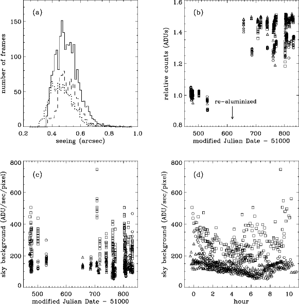
Figure 1: Shown are the raw data in the filters $J_{s}$ ($dotted\ line$ or $circles$), $H$ ($dashed\ line$ or $squares$), and $K_{s}$ ($solid\ line$ or $triangles$). (a) Histogram of the median seeing in the raw ISAAC images weighted by the weight function of Eq. 2 used to combine the images. (b) Relative instrumental counts in a $\approx 3\arcsec$ radius aperture of four bright non-saturated stars in individual sky-subtracted exposures, plotted against Julian Date. The relative increase in counts, slightly dependent on wavelength, after cleaning and re-aluminization of the mirror directly reflects the increase in efficiency of the telescope, because the sky background levels (c) remained the same. Presumably, the photons were scattered by dirt rather than absorbed before cleaning. (d) Nightly sky variations are largest and most rapid in the $H$-band and mean sky levels are highest at the beginning and ending of the night. $J_{s}$-band varies less and peaks at the start of the night, whereas $K$-band levels are most stable.

Our NIR imaging consists of a single ISAAC pointing centered on the WFPC2 main-field of the HDF-S ($\alpha=22^{h}32^{m}55.464$, $\delta=-60\arcdeg 33\arcmin 05.01\arcsec$, J2000) in the $J_{s}$, $H$ and $K_{s}$ filters, which gives good sampling of rest-frame optical wavelengths over the redshift range $1<z<4$. The $J_{s}$ filter is being established as the new standard broadband filter at $\approx 1.24\micron$ by most major observatories (Keck, Gemini, Subaru, ESO), and is photometrically more accurate than the classical $J$ because it is not cut off by atmospheric absorption. It is a top-hat filter with sharp edges, practically the same effective wavelength as the normal $J$ filter, and half-transmittance points at $1.17\micron$ and $1.33\micron$. We used the $K_{s}$ filter which is bluer and narrower than standard $K$, but gives a better signal-to-noise ratio (SNR) for faint sources because it is less affected by the high thermal background of the atmosphere and the telescope. The ISAAC $H$ and $K_{s}$ filters are close to those used to establish the faint IR standard star system (Persson et al., 1998), while the $J_{s}$ filter requires a small color correction. The WFPC2 filters that are used are $F300W,F450W,F606W$ and $F814W$ which we will call $U_{300}$, $B_{450}$, $V_{606}$ and $I_{814}$, respectively, where the subscript indicates the central wavelength in nanometers.

The observing strategy for the HDF-S follows established procedures for ground-based NIR imaging. The dominance of the sky background and its rapid variability in the infrared requires dithering of many short exposures. We used a $20\arcsec$ jitter box in which the telescope is moved in a random pattern of Poissonian offsets between successive exposures. This jitter size is a trade-off between keeping a large area at maximum depth and ensuring that each pixel has sufficient exposures on sky. Individual exposures have integration times of $6\times 30~{}$s in $J_{s}$, $6\times 20~{}$s in $H$, and $6\times 10~{}$s in $K_{s}$ (subintegrations $\times$ detector integration times). We requested service mode observations amounting to 32 hours in each band with a seeing requirement of $\lesssim 0\farcs 5$, seeing conditions that are only available 25% of the time at Paranal. The observations were grouped in $112$ observation blocks (OBs), each of which uniquely defines a single observation of a target, including pointing, number of exposures in a sequence, and filter. The calibration plan for ISAAC provides the necessary calibration measurements for such blocks, including twilight flats, detector darks, and nightly zero points by observing LCO/Palomar NICMOS standard stars (Persson et al., 1998).

2.2 Observations

The HDF-S was observed from October to December 1999 and from April to October 2000 under ESO program identification 164.O-0612(A). A summary of the observations is shown in 1. We obtained a total of $33.6$, $32.3$ and $35.6$ hours in $J_{s}$, $H$ and $K_{s}$, distributed over $33,34$ and $55$ OBs, or $1007,968$ and $2136$ frames, respectively. This represents all usable data, including aborted and re-executed OBs that were outside weather specifications or seeing constraints. In the reduction process these data are included with appropriate weighting (see section 3.4). Sixty-eight percent of the data was obtained under photometric conditions and the average airmass of all data was 1.25. A detailed summary of observational parameters with pointing, observation date, image quality and photometric conditions can be found on the FIRES homepage on the World Wide Web (http://www.strw.leidenuniv.nl/{̃}fires).

An analysis of various observational parameters reveals some surprising trends in the data, whereas other expected relations are less apparent. An overview is given in Figure 1. The median seeing on the raw images is better than 0$\farcs$5 in all bands, with the seeing of 90% of the images in the range $0\farcs 4-0\farcs 65$, as can be seen in Figure 1.

Seeing may vary strongly on short timescales but it is not related to any other parameter. The most drastic trend in the raw data is the change of sensitivity with date. Since the cleaning and re-alumization of the primary mirror in March 2000 the count rates of bright stars within a $\approx 3\arcsec$ aperture increased by $+29$% in $J_{s}$, $+45$% in $H$, and $+45$% $K_{s}$, which is reflected by a change in zero points before and after this date. Because the average NIR sky levels remained the same, this increase proportionally improved the achievable signal-to-noise for background-limited sources. The change in throughput was caused by light scattering, which explains why the sky level remained constant. Sky levels in $J_{s}$ and $H$, dominated by airglow from OH-emission lines in the upper atmosphere (typically 90 km altitude), vary unpredictably on the timescale of minutes, but also systematically with observed hour. The average sky level is highest at the beginning and end of each night with peak-to-peak amplitudes of the variation being 50% relative to the average sky brightnesses over the night. The background in $K_{s}$ is dominated by thermal emission of the telescope, instrument, and atmosphere and is mainly a function of temperature. The $K_{s}$ background is the most stable of all NIR bands and only weakly correlated with airmass; our data do not show a strong thermal atmospheric contribution, which should be proportional to atmospheric path length. We take into account the variations of the background and seeing through weighting in the data coadding process.

3 Data Reduction

The reduction process included the following steps: quality verification, flat-fielding, bad pixel correction, sky subtraction, distortion correction, registration, photometric calibration and weighting of individual frames, and combination into a single frame. We used a modified version of the DIMSUM package and standard routines in IRAF for sky subtraction and coadding, and the ECLIPSE package for creating the flatfields and the initial bad pixel masks. We reduced the ISAAC observations several times with an increasing level of sophistication, applying corrections to remove instrumental features, scattered light, or clear artifacts when required. Here we describe the first version of the reduction (v1.0) and the last version (v3.0), leaving out the intermediate trial versions. The last version produced the final $J_{s}$, $H$ and $K_{s}$ images, on which the photometry (see section 5) and analysis (see section 8) is based.

3.1 Flatfields and Photometric Calibration

We constructed flatfields from images of the sky taken at dusk or dawn, grouped per night and in the relevant filters, using the flat routine in ECLIPSE, which also provided the bad pixel maps. We excluded a few flats of poor quality and flats that exhibited a large jump between the top row of the lower and bottom row of the upper half of the array, possibly caused by the varying bias levels of the Hawaii detector. We averaged the remaining nightly flats per month, and applied these to the individual frames of the OBs taken in the same month. If no flatfield was available for a given month we used an average flat of all months. The stability of these monthly flats is very good and the structure changes little and in a gradual way. We estimate the relative accuracy to be $0.2-0.4$% per pixel from the pixel-to-pixel rms variation between different monthly flats. Large scale gradients in the monthly flats do not exceed 2%. We checked that standard stars, which were observed at various locations on the detector, were consistent within the error after flatfielding.

Standard stars in the LCO/Palomar NICMOS list (Persson et al., 1998) were observed each night, in a wide five-point jitter pattern. For each star, on each night, and in each filter, we measured the instrumental counts in a circular aperture of radius $20$ pixel ($2\farcs 94$) and derived zero points per night from the magnitude of that star in the NICMOS list. We identify non-photometric nights after comparison with the median of the zero points over all nights before and after re-aluminization in March 2000 (see section 2.2). The photometric zero points exhibit a large increase after March 2000 but, apart from this, the night-to-night scatter is approximately 2%. We adopted the mean of the zero points after March 2000 as our reference value. See Table 2 for the list of the adopted zero points. By applying the nightly zero points to 4 bright unsaturated stars in the HDF-S, observed on the same night under photometric conditions, we obtain calibrated stellar magnitudes with a night-to-night rms variation of only $\approx 1-1.5$%. No corrections for atmospheric absorption were required because the majority of the science data were obtained at similar airmass as the standard star observations. In addition, instrumental count rates of HDF-S stars in individual observation blocks reveal no correlation with airmass. We used the calibrated magnitudes of the 4 reference stars, averaged over all photometric nights, to calibrate every individual exposure of the photometric and non-photometric OBs. The detector non-linearity, as described by Amico et al. (2001), affects the photometric calibration by $\lesssim 1$% in the $H$-band, where the exposure levels are highest. Because the effect is so small, we do not correct for this. We did not account for color terms due to differences between the ISAAC and standard filter systems. Amico et al. (2001) report that the ISAAC $H$ and $K_{s}$ filters match very well those used to establish the faint IR standard star system of Persson et al. (1998). Only the ISAAC $J_{s}$ filter is slightly redder than Persson’s $J$ and this may introduce a small color term, $\approx-0.04\cdot(J-K)_{LCO}$. However, the theoretical transformation between ISAAC magnitudes and those of LCO/Palomar have never been experimentally verified. Furthermore, the predicted color correction is small and could not be reproduced with our data. In the absence of a better calibration we chose not to apply any color correction. We did apply galactic extinction correction when deriving the photometric redshifts, see section 6, but it is not applied to the catalog.

As a photometric sanity check, we compared $2\arcsec$ circular diameter aperture magnitudes of the brightest stars in the final (version 3.0, described below) images to magnitudes based on a small fraction of the data presented by R01. Each data set was independently reduced, the calibration based on different standard stars, and the shallower data were obtained before re-aluminization of the primary mirror. The magnitudes of the brightest sources in all bands agree within 1% between the versions, indicating that the internal photometric systematics are well under control. For the NIR data, the adopted transformations from the Johnson (1966) system to the AB system are taken from Bessell & Brett (1988) and we apply $J_{s,AB}=J_{s,Vega}+0.90,H_{AB}=H_{Vega}+1.38$ and $K_{s,AB}=K_{s,Vega}+1.86$.

3.2 Sky Subtraction and Cosmic Ray Removal

The rapidly varying sky, typically 25 thousand times brighter than the sources we aim to detect, is the primary limiting factor in deep NIR imaging. In the longest integrations, small errors in sky subtraction can severely diminish the achievable depth and affect faint source photometry. The IRAF package DIMSUM provides a two-pass routine to optimally separate sky and astronomical signal in the dithered images. We modified it to enable handling of large amounts of data and replaced its co-adding subroutine, which assumes that the images are undersampled, by the standard IRAF task IMAGES.IMMATCH.IMCOMBINE. The following is a brief summary of the steps performed by the REDUCE task in DIMSUM.

For every science image in a given OB a sky image is constructed. After scaling the exposures to a common median, the sky is determined at each pixel position from a maximum of 8 and a minimum of 3 adjacent frames in time. The lowest and highest values are rejected and the average of the remainder is taken as the sky value. These values are subtracted from the scaled image to create a sky subtracted image. A set of stars is then used to compute relative shifts, and the images are integer registered and averaged to produce an intermediate image. All astronomical sources are identified and a corresponding object mask is created. This mask is used in a second pass of sky subtraction where pixels covered by objects are excluded from the estimate of the sky.

The images show low-level pattern due to bias variations. Because they generally reproduce they are automatically removed in the skysubtraction step. We find cosmic rays with DIMSUM, using a simple threshold algorithm and replacing them by the local median, unless a pixel is found to have cosmic rays in more than frames per OB. In this case the pixel is added to the bad pixel map for that OB.

3.3 First Version and Quality Verification

The goal of the first reduction of the data set is to provide a non-optimized image, which we use to validate and to assess the improvements from more sophisticated image processing. The first version consists of registration on integer pixels and combination of the sky subtracted exposures per OB. For each of the $122$ OBs, we created an average and a median combined image to verify that cosmic rays and other outliers were removed correctly, and we visually inspected all $4149$ individual sky subtracted frames as well, finding that many required further processing as described in the following section. Finally, we generated the version 1.0 images (the first reduction of the full data set) by integer pixel shifting all OBs to a common reference frame, and coaveraging them into the $J_{s}$, $H$ and $K_{s}$ images. While this first reduction is not optimal in terms of depth and image quality, it is robust owing to its straightforward reduction procedure.

3.4 Additional Processing and Improvements

The individual sky subtracted frames are affected by a number of problems or instrumental features, which we briefly describe below, together with the applied solutions and additional improvements that lead to the version 3.0 images. The most important problems are:

• Detector bias residuals, most pronounced at the rows where the read-out of the detector starts at the bottom (rows $1,2,...$) and halfway (rows $513,514,...$), caused by the complex bias behaviour of the Rockwell Hawaii array. These variations are uniform along rows, and we removed the residual bias by subtracting the median along rows in individual sky subtracted exposures, after masking all sources.

• Imperfect sky subtraction, caused by stray light or rapid background variations. Strong variations in the backgrounds, reflection from high cirrus, reflected moonlight in the ISAAC optics or patterns of less obvious origin can lead to large scale residuals in the sky subtraction, particularly in $J_{s}$ and $H$. For some OBs, we succesfully removed the residual patterns by splitting the sequence in two (in case of a sudden appearance of stray light), or subtracting a two-piece cubic spline fit along rows and columns to the background in individual frames, after masking all sources. We rejected a few frames, or masked the affected areas, if this simple solution did not work.

• Unidentified cosmic rays or bad pixels. A small amount of bad pixels were not detected by ECLIPSE or DIMSUM routines but need to be identified because we average the final images without additional clipping or rejection. By combining the sky subtracted frames in a given OB without shifts and with the sources masked, we identified remaining cosmic rays or outliers through sigma clipping. We added $\sim 60-100$ pixels per OB to the corresponding bad pixel map.

Several steps were taken to improve the quality and limiting depths of the version 1.0 images, the most important of which are:

• Distortion correction of the individual frames and direct registration to the $3\times 3$ blocked $I_{814}$ image ($0.119\arcsec$pixel^-1), our preferred frame of reference. We obtained the geometrical distortion coefficients for the 3rd order polynomial solution from the ISAAC WWW-page. The transformation procedure involves distortion correcting the ISAAC images, adjusting the frame-to-frame shifts, and finding the linear transformation to the WFPC2 $I_{814}$ frame of reference. This linear transformation is the best fit mapping of source positions in the blocked WFPC2 $I_{814}$ image to the corresponding positions in the corrected $J_{s}$-band image. Compared to version 1.0 described in the previous section, this procedure increases registration accuracy and image quality, decreases image smearing at the edges introduced by the jittering and differential distortion. Given the small amplitude of the ISAAC field distortions, the effect on photometry is negligible. In the linear transformation and distortion correction step the image is resampled once using a third-order polynomial interpolation, with a minimal effect of the interpolant on the noise properties.

• Weighting of the images. We substantially improved the final image depth and quality by assigning weights to individual frames that take into account changes in seeing, sky transparency, and background noise. Two schemes were applied: one that optimizes the signal-to-noise ratio (SNR) within an aperture of the size of the seeing disk, and one that optimizes the SNR per pixel. The first improves the detection efficiency of point sources, the other optimizes the surface brightness photometry. The weights $w_{i}$ of the frames are proportional to either the inverse scaled variance $zpscale_{i}\times var_{i}$ within a seeing disk of size $s_{i}$, or to the inverse scaled variance per pixel, where the scaling $zpscale_{i}$ is the flux calibration applied to bring the instrumental counts of our four reference stars in the HDF-S to the calibrated magnitude.

  $$w_{i,point}\propto(zpscale_{i}\times var_{i}\times s^{2}_{i})^{-1}$$ (1)

  $$w_{i,extended}\propto(zpscale_{i}\times var_{i})^{-1}$$ (2)

3.5 Final Version and Post Processing

The final combined $J_{s}$, $H$, and $K_{s}$ images (version 3.0) were constructed from the individually registered, distortion corrected, weighted and unclipped average of the $1007,\ 968$, and $2136$ NIR frames respectively. Ultimately, less than 3% of individual frames were excluded in the final images because of poor quality. In this step we also generated the weight maps, which contain the weighted exposure time per pixel. We produced three versions of the images, one with optimized weights for point sources, one with optimized weights for surface brightness, and one consisting of the best quartile seeing fraction of all exposures, also optimized for point sources. The weighting has improved the image quality by 10–15% and the background noise by 5–10%, and distortion correction resulted in subpixel registration accuracy between the NIR images and $I_{814}$-band image over the entire field of view.

The sky subtraction routine in DIMSUM and our additional fitting of rows and columns (see section 3.4) have introduced small negative biases in combined images, caused by systematic oversubtraction of the sky which was skewed by light of the faint extended PSF wings or very faint sources, undetectable in a single OB. Because of this, the flatness of the sky on large scales was limited to about 10^-5. The negative bias was visible as clearly defined orthogonal stripes at P.A.$\approx 6\arcdeg$, as well as dark areas around the brightest stars or in the crowded parts of the images. To solve this, we rotated a copy of the final images back to the orientation in which we performed sky substraction, fitted a 3-piece cubic spline to the background along rows and columns (masking all sources), re-rotated the fit, and subtracted it. The sky in the final images is flat to a few $\times 10^{-6}$ on large ($>20\arcsec$) scales.

4 Final Images

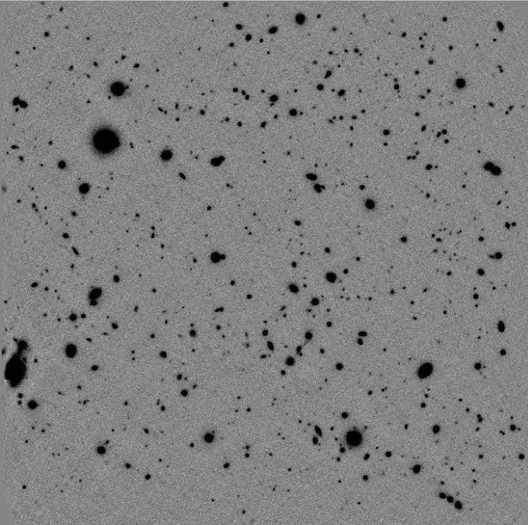
Figure 2: The HDF-S field in the ISAAC $K_{s}$-band divided by the square root of the weight map (based on the fractional exposure time per pixel) and displayed at linear scaling. The total integration time is 35.6 hours, the stellar FWHM$\approx 0\farcs 46$ and the total field size is $2.85\arcmin\times 2.85\arcmin$.

The reduced NIR $J_{s}$, $H$, and $K_{s}$ images and weight maps can be obtained from the FIRES-WWW homepage (http://www.strw.leidenuniv.nl/{̃}fires). Throughout the rest of the paper we will only consider the images optimized for point source detection which we will use to assemble the catalog of sources.

4.1 Properties

The pixel size in the NIR images equals that of the $3\times 3$ blocked WFPC2 $I_{814}$-band image at $0.119\arcsec$ pixel^-1. The combined ISAAC images are aligned with the HST version 2 images (Casertano et al., 2000) with North up, and are normalized to instrumental counts per second. The images are shallower near the edges of the covered area because they received less exposure time in the dithering process, which is reflected in the weight map containing the fraction of total exposure time per pixel. The area of the ISAAC $K_{s}$-band image with weight per pixel $w_{K}\geq 0.95,0.2,$ and $0.01$ covers $4.5,7.2$ and $8.3$ arcmin², while the area used for our preferred quality cut for photometry ($w\geq 0.2$ in all seven bands) is $4.7$ arcmin². The NIR images have been trimmed where the relative exposure time per pixel is less than 1%.

Figure 2 shows the noise-equalized $K_{s}$-detection image obtained by division with the square root of the exposure-time map. The richness in faint compact sources and the flatness of the background are readily visible. Figure 3 shows a RGB color composite image of the $I_{814}$, $J_{s}$, and $K_{s}$ images. The PSF of the space-based $I_{814}$ image has been matched to that of the NIR images at FWHM$\approx 0\farcs 46$ (see section 4.2) and three adjacent WFPC2 $I_{814}$ flanking fields have been included for visual purposes. We set the linear stretch of both images to favor faint objects. Immediately striking is the rich variety in optical-NIR colors, even for the faint objects, indicating that the NIR observations are very deep and that there is a wide range of observed spectral shapes, which can result from different types of galaxies over a broad redshift range.

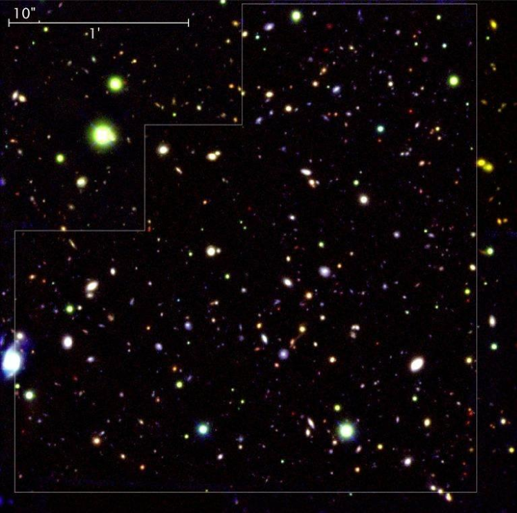
Figure 3: Three-color composite image of the ISAAC field on top of the WFPC2 main-field and parts of three WFPC2 flanking fields. The main-field is outlined in white and North is up. The images are registered and smoothed to a common seeing of FWHM$\approx 0\farcs 46$, coding WFPC2 $I_{814}$ in blue, ISAAC $J_{s}$ in green and ISAAC $K_{s}$ in red. There is a striking variety in optical-to-infrared colors, especially for fainter objects. A number of sources with red colors have photometric redshifts $z>2$ and they are candidates for relatively massive, evolved galaxies. These galaxies would not be selected by the U-dropout technique because they are too faint in the observer’s optical.

4.2 Image Quality

The NIR PSF is stable and symmetric over the field with a gaussian core profile and an average ellipticity $<0.05$ over the $J_{s}$, $H$, and $K_{s}$ images. The median FWHM of the profiles of ten selected isolated bright stars is $0\farcs 45$ in $J_{s}$, $0\farcs 48$ $H$, and $0\farcs 46$ $K_{s}$  with $0\farcs 04$ amplitude variation over the images.

For consistent photometry in all bands we convolved the measurement images to a common PSF, corresponding to that of the $H$-band which had worst effective seeing (FWHM $=0\farcs 48$). The similarity of PSF structure across the NIR images allowed simple gaussian smoothing for a near perfect match. The complex PSF structure of the WFPC2 requires convolving with a special kernel, which we constructed by deconvolving an average image of bright isolated non-saturated stars in the $H$-band with the average $I_{814}$-band image of the same stars. Division of the stellar growth curves of the convolved images by the $H$-band growth curve shows that the fractional enclosed flux agrees to within 3% at radii $r\geq 0\farcs 35$.

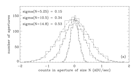
Figure 4: Scaling relation of the measured background rms noise as a function of linear size $N=\sqrt{A}$ of apertures with area A. (a) Gaussians are fitted to histograms of $K_{s}$ counts in randomly placed apertures of increasing size, excluding pixels belonging to sources. This correctly accounts for pixel-to-pixel correlations and other effects, allowing us to measure the true rms variation as a function of linear size of aperture. (b) The $K_{s}$-band results (solid points), together with the best-fit scaling relation of Eq. 3 (solid line), show that the measured variation in large apertures exceeds the variation expected from linear (Gaussian) scaling of the pixel-to-pixel noise (dashed line), likely due to large scale correlated fluctuations of the background.

4.3 Astrometry

The relative registration between ISAAC and WFPC2 images needs to be very precise, preferably a fraction of an original ISAAC pixel over the whole field of view, to allow correct cross-identification of sources, accurate color information and morphological comparison between different bands. To verify our mapping of ISAAC to WFPC2 coordinates, we measured the positions of the 20 brightest stars and compact sources in all registered ISAAC exposures, and we compared their positions with those in the $I_{814}$ image. The rms variation in position of individual sources is about $0.2-0.3$ pixel at $0.119\arcsec$ pixel^-1 ($25-35$ mas), but for some sources systematic offsets between the NIR and the optical up to $0.85$ pixel ($100$ mas) remain. The origin of the residuals is unclear and we cannot fit them with low order polynomials. They could be real, intrinsic to the sources, or due to systematic errors in the field distortion correction of ISAAC or WFPC2. However, for all our purposes, the effect of positional errors of this amplitude is unimportant. The error in absolute astrometry of the HST HDF-S coordinate system, estimated to be less than $40$ mas, is dominated by the systematic uncertainty in the positions of four reference stars (Casertano et al., 2000; Williams et al., 2000).

4.4 Backgrounds and Limiting Depths

The noise properties of the raw individual ISAAC images are well described by the variance of the signal collected in each pixel since both Poisson and read noise are uncorrelated. However, image processing, registration and combination have introduced correlations between neighbouring pixels and small errors in the background subtraction may also contribute to the noise. Understanding the noise properties well is crucial because limiting depths and photometric uncertainties rely on them.

Instead of a formal description based on the analysis of the covariance of correlated pixel pairs, we followed an empirical approach where we fit the dependence of the rms background variation in the image as a function of linear size $N=\sqrt{A}$ of apertures with area $A$. Directly measuring the effective flux variations in apertures of different sizes provides a more realistic estimate of signal variations than formal Gaussian scaling $\sigma(N)=N\bar{\sigma}$ of the pixel-to-pixel noise $\bar{\sigma}$, as is often done.

We measured fluxes in $1200$ non-overlapping circular apertures randomly placed on the registered convolved images, which were also used for photometry. We excluded all pixels belonging to sources detectable in $K_{s}$ at the 5$\sigma$ level (see section 5.1 for detection criteria). We used identical aperture positions for each band $i$ and measured fluxes for circular aperture diameters ranging from $0\farcs 5$ to $3\arcsec$. Then we obtained the flux dispersions by fitting a Gaussian distribution to the histogram of fluxes at each aperture size. Finally, we fitted a parameterized function of linear size to the different dispersions:

$$\sigma_{i}(N)=N\bar{\sigma}_{i}(a_{i}+b_{i}N)/\sqrt{w_{i}}$$ (3)

This equation describes the signal variation versus aperture size $N$ over the entire image, taking into account spatial variations as a result of relative weight $w_{i}$ for each passband $i$. As can be seen in Figure 4, it provides a good fit to the noise characteristics. The noise is significantly higher than expected from uncorrelated (Gaussian) noise, indicated by a dashed line in Figure 4b. Table 3 shows the best fit values in all bands and the corresponding limiting depths. The parameter $a$ reflects the correlations of neighbouring pixels ($a>1$), which is important in the WFPC2 images because of heavy smoothing, but also in the ISAAC images given the resampling from $0\farcs 147$ to $0\farcs 119$ pixel^-1. The parameter $b$ accounts for large scale correlated variations in the background ($b>0$). This may be caused by the presence of sources at very faint flux levels (confusion noise) or instrumental features. Typically, the large scale correlated contribution per pixel is only 3-15% relative to the gaussian rms variation, but due to the $N^{2}$ proportionality the contribution to the variation in large apertures increases to significant levels. While the signal variations grow faster with area than expected from a Gaussian, at any specific scale the variation is consistent with a pure Gaussian.

From the analysis of the scaling relation of simulated colors we find that part of the large scale irregularities in the background are spatially correlated between bands. In particular, we measured the rms variation of the $I_{814}-V_{606}$ colors directly by subtracting in registered apertures the $I_{814}$-band fluxes from the $V_{606}$ fluxes and fitting the dispersion of the difference at each linear size. On large scales rms variations are 30% smaller than predicted from Eq. 3 if the noise were uncorrelated. Yet, if we subtract the two fluxes in random apertures, the scaling of the background variation is consistent with the prediction. A similar effect is seen for the $I_{814}-J_{s}$ color, but at a smaller amplitude. The spatial coherence of the background variations between filters and across cameras suggests that part of the background fluctuations may be associated with sources at very faint flux levels. Other contributions are likely similar flatfielding or skysubtraction residuals from one band to another.

5 Source Detection and Photometry

The detection of sources at very faint magnitudes against a noisy background forces us to trade off completeness and reliability. A very low detection threshold may generate the most complete catalog, but we must then apply additional criteria to assess the reliability of each detection given that such a catalog will contain many spurious sources. More conservatively, we choose the lowest possible threshold for which contamination by noise is unimportant. We aim to produce a catalog with reliable colors suitable for robustly modeling of the intrinsic spectral energy distribution. Using SExtractor version 2.2.2 (Bertin & Arnouts, 1996) with a detection procedure that optimizes sensitivity for point-like sources, we construct a $K_{s}$-band selected catalog with seven band optical-to-infrared photometry.

5.1 Detection

To detect objects with SExtractor using a constant signal-to-noise criterion over the entire image, including the shallower outer parts, we divide the point source optimized $K_{s}$-image by the square root of the weight (exposure time) map to create a noise-equalized detection image. A source enters the catalog if, after low-pass filtering of the detection image, at least one pixel is above $\approx 5$ times the standard deviation of the filtered background, corresponding to a total $K_{s}$-band magnitude limit for point sources of $K_{s}\approx 26.0$. This depth is reached for the central $4.5$ arcmin². In total we have 833 detections in the entire survey area of $8.3$ arcmin². Initially 820 sources are found but the detection software fails to detect sources lying in the extended wings of the brightest objects. To include these, we fit the surface brightness profiles of the brightest sources with the GALPHOT package (Franx et al., 1989) in IRAF, subtract the fit, and carry out a second detection pass with identical parameters. Thirteen new objects enter the catalog, and 9 sources detected in the first pass are replaced with improved photometry. The catalog identification numbers of all second-pass objects start at 10001, and the original entries of the updated sources are removed.

Filtering affects only the detection process and the isophotal parameters; other output parameters are affected only indirectly through barycenter and object extent. We chose a simple two-dimensional gaussian detection filter (FWHM$=0\farcs 46$), approximating the core of the effective $K_{s}$-band PSF well. Hence, we optimize detectability for point-like sources, introducing a small bias against faint extended objects. In principle it is possible to combine multiple catalogs created with different filter sizes but merging these catalogs consistently is a complicated and subjective process yielding a modest gain only in sensitivity for larger objects. We prefer the small filter size equal to the PSF in the detection map because the majority of faint sources that we detect are compact or unresolved in the NIR and because we wish to minimize the blending effect of filtering on the isophotal parameters and on the confusion of sources. SExtractor applies a multi-thresholding technique to separate overlapping sources based on the distribution of the filtered $K_{s}$-band light. About 20% of the sources are blended because of the low value of the isophotal threshold; in SExtractor this must always equal the detection threshold. With the deblending parameters we used, the algorithm succeeds in splitting close groups of separate galaxies, without “oversplitting” galaxies with rich internal structure.

We tested sensitivity to false detections by running SExtractor on a specially constructed $K_{s}$-band noise map created by subtracting, in pairs, individual $K_{s}$-band images of comparable seeing, after zero point scaling, and coaveraging the weighted difference images. This noise image has properties very similar to the noise in the original reduced image, including contributions from the detector and reduction process, but with no trace of astronomical sources. Our detection algorithm resulted in only 11 spurious sources over the full area.

5.2 Optical and NIR Photometry

We use SExtractor’s dual-image mode for spatially accurate and consistent photometry, where objects are detected and isophotal parameters are determined from the $K_{s}$-band detection image while the fluxes in all seven bands are measured in the registered and PSF matched images. We used fluxes measured in circular apertures $APER(D)$ with fixed-diameters $D$, isophotal apertures $APER(ISO)$ determined by the $K_{s}$-band detection isophote at the $5\sigma$ detection threshold, and $APER(AUTO)$ (autoscaling) apertures inspired by Kron (1980), which scales an elliptical aperture based on the first moments of the $K_{s}$-band light distribution. We select for each object the best aperture based on simple criteria to enable detailed control of photometry. We define two types of measurements:

• “color” flux, to obtain consistent and accurate colors. The optimal aperture is chosen based on the $K_{s}$ flux distribution, and this aperture is used to measure the flux in all other bands.

• “total” flux, only in the $K_{s}$-band, which gives the best estimate of the total $K_{s}$ flux.

For both measurements we treat blended sources differently from unblended ones, and consider a source blended when its BLENDED or BIAS flag is set by SExtractor, as described in Bertin & Arnouts (1996).

Our color aperture is chosen as follows, introducing the equivalent of a circular isophotal diameter $D_{iso}=2\sqrt{A_{iso}/\pi}$ based on $A_{iso}$, the measured non-circular isophotal area within the detection-isophote:

$$\begin{array}[]{lcl}\text{if the source is {\it not} blended}&&\\ &&\\ APER(COLOR)=\begin{cases}APER(ISO)&(0\farcs 7<D_{iso}<2\farcs 0)\\ APER~{}(0\farcs 7)&(D_{iso}\leq 0\farcs 7)\\ APER~{}(2\farcs 0)&(D_{iso}\geq 2\farcs 0)\\ \end{cases}&&\\ &&\\ \text{else if the source is blended}&&\\ &&\\ APER(COLOR)=\begin{cases}APER~{}(D_{iso}/s)&(0\farcs 7<D_{iso}/s<2\farcs 0)\\ APER~{}(0\farcs 7)&(D_{iso}/s\leq 0\farcs 7)\\ APER~{}(2\farcs 0)&(D_{iso}/s\geq 2\farcs 0)\\ \end{cases}&&\\ \end{array}$$ (4)

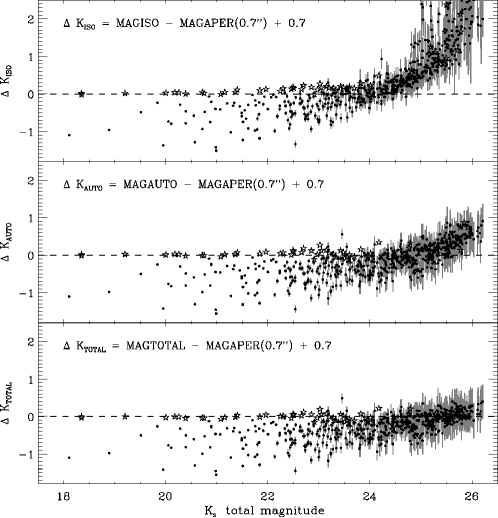
Figure 5: Comparison of methods to estimate total $K_{s}$-band magnitude. Shown are isophotal (top), SExtractor’s auto-scaling AUTO (middle), and our “total” magnitudes (bottom) as defined in Eq. 5 and which are aperture corrected using stellar growth curve analysis. We subtracted the aperture corrected magnitude measured in an aperture of $0\farcs 7$ ($MAGAPER(0\farcs 7)-0.7$), which produces the correct total magnitudes for stars and pointlike sources. Stars are marked by star symbols and fluxes are plotted with $\pm 1\sigma$ error bars. The turn-up at $K_{s}\approx 24$ of isophotal and at $K_{s}\approx 25$ of the AUTO magnitudes shows that these photometric schemes systematically underestimate the total flux at faint levels, due to the decreasing size of the used aperture with magnitude. This effect is nearly absent in the bottom panel, which shows the total magnitudes measured in this paper.

The parameter $s$ is the factor with which we shrink the circular apertures centered on blended sources, increasing the separation to the blended neighbour such that mutual flux contamination is minimal. This factor depends on the data set, and for our ISAAC $K_{s}$ image we find that $s=1.4$ is most successful. The smallest aperture considered, APER($0\farcs 7$), $\approx 1.5$ FWHM of the effective PSF, optimizes the S/N for photometry of point sources in unweighted apertures and prevents smaller more error-prone apertures. The largest allowed aperture, APER($2\farcs 0$), prevents large and inaccurate isophotal apertures driven by the filtered $K_{s}$-light distribution. We continuously assessed the robustness and quality of color flux measurements by inspecting the fits of redshifted galaxy templates to the flux points, as described in detail in $\S$6.

We calculate the total flux in the $K_{s}$-band from the flux measured in the AUTO aperture. We define a circularized AUTO diameter $D_{auto}=2\sqrt{A_{auto}/\pi}$ with $A_{auto}$ the area of the AUTO aperture, and define the total magnitude as:

$$\begin{array}[]{lcl}\text{if the source is {\it not} blended}&&\\ &&\\ APER(TOTAL)=APER(AUTO)&&\\ &&\\ \text{else if the source is blended}&&\\ &&\\ APER(TOTAL)=APER(COLOR)&&\\ &&\\ \end{array}$$ (5)

Finally, we apply an aperture correction using the growth curve of brighter stars to correct for the flux lost because it fell outside the “total” aperture. This aperture correction is necessary because it is substantial for our faintest sources, as shown in Figure 5 where we compare different methods to estimate magnitude. The aperture correction reaches 0.7 mag at the faint end, therefore magnitudes are seriously underestimated if the aperture correction is ignored.

We derive the $1\sigma$ photometric error for all measurements from Eq. 3 with the best-fit values shown in Table 3. These errors may overestimate the uncertainty in colors of adjacent bands (see section 4.4) but it should represent well the photometric error over the entire $0.3\mu-2.2\micron$ wavelength range. The magnitudes may suffer from additional uncertainties because of surface brightness biases or possible biases in the sky subtraction procedure which could depend on object magnitude and size.

6 Photometric Redshifts

To physically interpret the seven-band photometry for our $K_{s}$-band selected sample, we use a photometric redshift ($z_{phot}$) technique explained in detail by R01. In summary, we correct the observed flux points for galactic extinction (see Schlegel, Finkbeiner, & Davis 1998) and we model the rest-frame colors of the galaxies by fitting a linear combination of redshifted empirical galaxy templates. The redshift with the lowest $\chi^{2}$ statistic, where

$$\chi^{2}(z)=\sum^{N_{filter}}_{i=1}\left[\frac{F_{i}^{data}-F_{i}^{model}}{\sigma_{i}^{data}}\right]^{2}$$ (6)

is then chosen as the most likely $z_{phot}$. Using a linear combination of SEDs as $F^{model}$ minimizes the a priori assumptions about the nature and stellar composition of the detected sources.

Our data set with three deep NIR bands samples the position of Balmer/4000Å break over $1\lesssim z\lesssim 4$, allowing us to probe the redshift distribution of more evolved galaxy types that may have little rest-frame UV flux and hence a weak or virtually absent Lyman break.

Figure 6: Direct comparison of photometric redshifts to the 39 spectroscopic redshifts of objects in the HDF-S with good photometry in all bands. The 68% error bars are derived from our Monte Carlo simulations and the diagonal line corresponds to a one-to-one relation to guide the eye. While the agreement is excellent with no failures for this small sample and with mean $\Delta z/(1+z)=0.08$, large asymmetric uncertainties remain for some objects indicating the presence of a second photometric redshift solution of comparable likelihood at a different redshift.

6.1 Photometric Templates

We used the local Hubble type templates E, Sbc, Scd, and Im from Coleman, Wu, & Weedman (1980), the two starburst templates, SB1 and SB2, with low derived reddening from Kinney et al. (1996), and a 10 Myr old single age template model from Bruzual & Charlot (2002). The starburst templates are needed because many galaxies even in the nearby Universe have bluer colors than the bluest CWW templates. The observed templates are extended beyond their published wavelengths into the far-ultraviolet by power law extrapolation and into the NIR using stellar population synthesis models from Bruzual & Charlot (2002), with the initial mass functions and star-formation timescales for each template Hubble type from Pozzetti, Bruzual, & Zamorani (1996). We accounted for internal hydrogen absorption of each galaxy by setting the flux blueward of the $912$Å Lyman limit to zero, and for the redshift-dependent cosmic mean opacity due to neutral intergalactic hydrogen by following the prescriptions of Madau (1995).

6.2 $Z_{phot}$ Uncertainties

The best test of photometric redshifts is direct comparison to spectroscopic redshifts, but spectroscopic redshifts in the HDF-S are still scarce. We calculate the uncertainty in the photometric redshift due to the flux measurement errors using a Monte-Carlo (MC) technique derived from that used in R01 and fully explained in Rudnick et al. (2002b). At bright magnitudes template mismatch dominates the errors, something that is not modeled by the MC simulation. Hence, the MC error bars for bright galaxies are severe underestimates. At fainter magnitudes, the uncertainty is driven by errors in photometry (Fernández-Soto, Lanzetta, & Yahil, 1999) and the MC technique should provide accurate $z_{phot}$ uncertainties. Experience from R01 showed that two ways to correct for the template mismatch, setting a minimum fractional flux error or setting a minimum $z_{phot}$ error based on the mean disagreement with $z_{spec}$, either degrade the accuracy of the $z_{phot}$ measurement or reflect the systematic error only in the mean, while template mismatch can be a strong function of SED shape and redshift. A method based completely on Monte-Carlo techniques is preferable because it has a straightforwardly computable redshift probability function. This approach is desirable for estimating the rest-frame luminosities and colors (Rudnick et al., 2002b).

Therefore, we modify the MC errors directly using the FIRES photometry. In summary, we estimate the systematic component of the $z_{phot}$ uncertainty by scaling up all the photometric errors for a given galaxy with a constant to bring residuals of the fit in agreement with the errors. This will not change the best fit redshift and SED and will not modify the MC errorbars of faint objects, but it will enlarge the redshift interval over which the templates can satisfactorily fit the bright objects. Only in case of widely different photometric errors between the visible and infrared might the modified MC uncertainties still underestimate the true $z_{phot}$ uncertainty.

In Figure 6 we show a direct test of photometric redshifts of the 39 objects in the HDF-S with available spectroscopy and good photometry in all bands. The current set of spectroscopic redshifts in the HDF-S will appear in Rudnick et al. (2002a). For the small sample that we can directly compare, we find excellent agreement with no failures and with a mean $\Delta z/(1+z_{spec})\approx 0.08$ with $\Delta z=|z_{spec}-z_{phot}|$. It is encouraging to see that the modified 68% error bars that were derived from the Monte Carlo simulations are consistent with the measured disagreement between $z_{phot}$ and the $z_{spec}$ in the HDF-S. However, large asymmetric uncertainties remain for some objects, clearly showing the presence of a second photometric redshift solution of comparable likelihood at a vastly different redshift, revealing limits on the applicability of the photometric redshift technique.

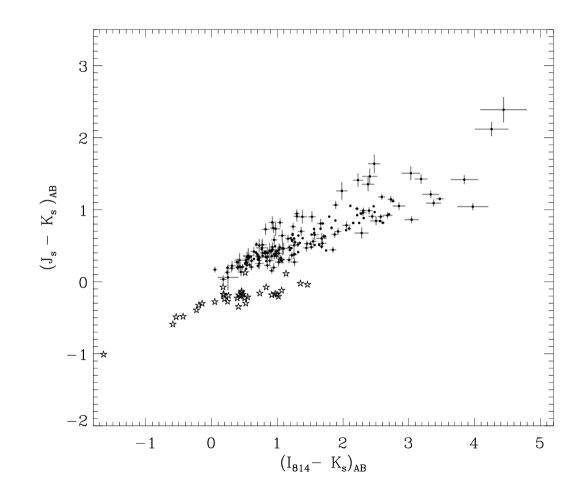
Figure 7: $J_{s}-K_{s}$ versus $I_{814}-K_{s}$ color-color diagram (on the AB system) for the sources with $K_{s}<24$ in the HDF-S with a minimum of 20% of the total exposure time in all bands. Identified stars are marked by a star symbol. The colors are plotted with $\pm 1\sigma$ error bars. There is a large variation in both $I-K_{s}$ and $J_{s}-K_{s}$ colors. Redshifted galaxies are well separated from the stellar locus in color-color space.

6.3 Stars

In a pencil beam survey at high Galactic latitude such as the HDF-S, a limited number of foreground stars are expected. We identify stars as those objects which have a better raw $\chi^{2}$ for a single stellar template fit than the $\chi^{2}$ for the galaxy template combination. The stellar templates are the NEXTGEN model atmospheres from Hauschildt et al. (1999) for main sequence stars with temperatures of $3000$ to $10000$K, assuming local thermodynamical equilibrium (LTE). Models of cooler and hotter stars cannot be included because non-LTE effects are important. We checked the resulting list of stars using the FWHM in the original $B_{450}$-band image and the $J_{s}-K_{s}$ color, excluding two objects (catalog IDs 207 and 296) that were obviously extended in $B_{450}$, and we find a total of 57 stars. As shown in Figure 7, most galaxies are clearly separated from the stellar locus in $I_{814}-K_{s}$ versus $J_{s}-K_{s}$ color-color space. Other cooler stars might still resemble SEDs of redshifted compact galaxies but the latter are generally redder in the infrared $J_{s}-K_{s}$ than most known M or methane dwarfs. Known cool L-dwarfs fall along a redder extension of the track traced by M-dwarfs in color-color space and have progressively redder $J_{s}-K_{s}$ colors for later spectral types. However measurements by Kirkpatrick et al. (2000) show the L-dwarf sequence abruptly stopping at $(J_{s}-K_{s})_{J}\approx 2.1$ (the subscript noting Johnson magnitudes, see section 3.1 for the transformations to the AB system) whereas even cooler T-dwarfs have much bluer $(J_{s}-K_{s})_{J}\approx 0$ colors than expected from their temperatures due to strong molecular absorption. This is important because if we would apply a $(J_{s}-K_{s})_{J}>2.3$ photometric criterion to select $z>2$ galaxies (as discussed in section 8.2), then we should ensure that cool Galactic stars are not expected in such a sample. The published data on the lowest-mass stars suggest that they are too blue in infrared colors to be selected this way. Only heavily reddened stars with thick circumstellar dust shells, such as extreme carbon stars or Mira variables, or extremely metal-free stars having a hypothetical $\lesssim 1500$K blackbody spectrum could also have red $(J_{s}-K_{s})_{J}>2.3$ colors but it seems unlikely that the tiny field of the HDF-S would contain such unusual sources.

Figure 8: Completeness curves (on the AB system) for the detectability of point sources in $J_{s}$ (triangles) and $K_{s}$ (points), based on simulations where we calculated the recovered fraction of stars that were dimmed to magnitudes between $22$ and $28$ and embedded in the survey images. The detection threshold of the source extraction software was set to $3.5\sigma$ of the filtered background rms. The dotted lines indicate the 50% and 90% completeness levels.

7 Catalog Parameters

The $K_{s}$-selected catalog of sources is published electronically. We describe here a subset of the photometry containing the most important parameters. The catalog with full photometry and explanation can be obtained from the FIRES homepage .

• $ID$. — A running identification number in catalog order as reported by SExtractor. Sources added in the second detection pass have numbers higher than 10000.

• $x,y$. — The pixel positions of the objects corresponding to the coordinate system of the original (unblocked) WFPC2 version 2 images.

• $RA,DEC$. – The right ascension and declination in equinox J2000.0 coordinates of which only the minutes and seconds of right ascension, and negative arcminutes and arcseconds of declination are given. To these must be added $22^{h}$(R.A.) and $-60\arcdeg$(DEC).

• $f_{col,i}\pm\sigma_{i}$. — The sum of counts in the “color” aperture $f_{col,i}$ in band $i=\{U_{300},B_{450},V_{606},I_{814},J_{s},H,K_{s}\}$ and its simulated uncertainty $\sigma_{i}$, as described in $\S$ 5.2. The fluxes are given in units of $10^{-31}$ ergs s^-1 Hz^-1 cm^-2.

• $K_{tot}\pm\sigma(K_{tot})$. — Estimate of the total $K_{s}$-band flux and its uncertainty. The sum of counts in the “total” aperture is corrected for missing flux assuming a PSF profile outside the aperture, as described in $\S$ 5.2.

• $ap\_col$. — An integer encoding the aperture type that was used to measure $f_{col,i}$. This is either a (1) $0\farcs 7$ diameter circular aperture, (2) $2\farcs 0$ diameter circular aperture, (3) isophotal aperture determined by the detection-image isophote, or a (4) circular aperture with a reduced isophotal diameter $D=\sqrt{(A_{iso}/\pi)}/1.4$.

• $ap\_tot$. — An integer encoding the aperture type that was used to measure $K_{tot}$. This is either a (1) automatic Kron-like aperture, or a (2) circular aperture within a reduced isophotal diameter.

• $r_{col},r_{tot}$. — Circularized radii $r=\sqrt{A/\pi}$, corresponding to the area $A$ of the specified “color” or “total” aperture.

• $A_{iso},A_{auto}$. — Area of the detection isophote $A_{iso}$ and area of the autoscaling elliptical aperture $A_{auto}=\pi*a*b$ with semi-major axis $a$ and semi-minor axis $b$.

• $FWHM_{K},FWHM_{I}$. — Full width at half maximum of a source in the $K_{s}$ detection image $FWHM_{K}$, and that of the brightest $I_{814}$-band source that lies in its detection isophote $FWHM_{I}$. We obtained the latter by running SExtractor separately on the original $I_{814}$-image and cross correlating the $I_{814}$-selected catalog with the $K_{s}$-limited catalog.

• $w_{i}$. — The weight $w_{i}$ represents, for each band $i$, the fraction of the total exposure time at the location of a source.

• $flags$.— Three binary flags are given. The $bias$ flag indicates either that the AUTO aperture measument is affected by nearby sources, or marks apertures containing more than 10% bad pixels. The $blended$ flag indicates overlapping sources, while the $star$ flag shows that the source SED is best fit with a stellar template (see section 6.3).

Figure 9: Differential $K_{s}$-band counts (on the AB system) of galaxies in the HDF-S. The counts are based on auto-scaling apertures (Kron, 1980) for isolated sources and adapted isophotal apertures for blended sources, both corrected to total magnitudes using stellar growth curve measurements. Raw counts (open circles) and counts corrected for incompleteness and false positive detections using point source simulations (filled circles) are shown. The small corrections at magnitudes $\gtrsim 23$ reflect missed sources due to confusion. Effective corrections at the faintest magnitudes $K_{s}\sim 25-25.5$ are very small because the loss of sources on negative noise regions (incompletenesss) is compensated by the number of sources pushed above the detection limit by positive noise fluctuations. Only the faintest $0.5$ mag bin centered on $K_{s}=26.0$, bordering the $3.5\sigma$ detection limit ($K_{s}\approx 26.3$), is significantly corrected because of a contribution of false positive detections.

8 Analysis

8.1 Completeness and Number Counts

The completeness curves for point-sources in the $J_{s}$ and $K_{s}$-band as a function of input magnitude are shown in Figure 8. Our 90% and 50% completeness levels on the AB magnitude system are $25.65$ and $26.25$, respectively, in $K_{s}$, and $26.30$ and $26.90$ in $J_{s}$.

We derived the limits from simulations where we extracted a bright non-saturated star from the survey image and add it back $30000$ times at random locations, applying a random flux scaling drawn from a rising count slope (or an increasing surface density of galaxies with magnitude) to bring it to magnitudes between $22\leq K_{s,AB}\leq 28$. We added the dimmed stars back in series of $30$ realizations so that they do not overlap each other. The rising count slope needs to be considered because the slope influences the number of recovered galaxies per apparent magnitude, as described below. The input count slope is based on the observed surface densities in the faint magnitude range where the signal-to-noise is $60\lesssim SNR\lesssim 10$ (or $23\lesssim K_{s,tot}\lesssim 25$) and where incompleteness does not yet play a role. We used only the deepest central $4.5$ arcmin² of the $J_{s}$  and $K_{s}$ images ($w>0.95$) with near uniform image quality and exclude four small regions around the brightest stars. In the simulation images we extract sources following the same procedures as described in $\S$5.1, but applying a reduced ($\approx 3.5\sigma$) detection threshold. We measure the recovered fraction of input sources against apparent magnitude, and from this we estimate the detection efficiency of point-like sources which we use to correct the observed number counts. We executed this procedure in the $J_{s}$ and $K_{s}$-band.

The resulting completeness curves assume that the true profile of the source is point-like and therefore they should be considered upper limits. An extended source would have brighter completeness limits depending on the true source size, its flux profile, and the filter that is used in the detection process. However, the detailed treatment of detection efficiency as a function of source morphology and detection criteria is beyond the scope of this paper.

When using the completeness simulations to correct the number counts, we choose a simple approach and apply a single correction down to $\approx 50$% completeness, based on the ratio of the simulated counts per input magnitude bin to the total recovered counts per observed total magnitude bin. More sophisticated modeling is possible but requires detailed knowledge of the intrinsic size and shape distribution of faint NIR galaxies. The simple approach corrects for all effects resulting from detection criteria, photometric scheme, incompleteness, and noise peaks. We find it works well if the total magnitude of sources is measured correctly, with little systematic difference between the input and recovered magnitudes, which is the case for our photometric scheme (see section 5.2). It is worth noticing that at $K_{s,AB}>25$ we actually recovered slightly more counts in the observed magnitude bins than we put in. This is caused by the fact that, in the case of a rising count slope, there are more faint galaxies boosted by positive noise peaks than bright galaxies lost on negative noise peaks. This effect is strong at low signal-to-noise fluxes and results in a slight excess of recovered counts. This is the main reason that we required little correction up to the detection threshold, except for the faintest $0.5$ mag bin centered on $K_{s}=26.0$, which contained false positive detections due to noise. After removing stars (see section 6.3), we plot in Figure 9 the raw and corrected source counts against total magnitude.

Figure 10: FIRES $K_{s}-$band galaxy counts (on the conventional Johnson system) compared to published counts in deep $K$-band fields. The corrected counts (filled circles) are shown for FIRES data. The Maihara et al. (2001) counts have been plotted to their S/N$\sim 3$ limit. The slope at magnitudes $K_{J}>21$ is flatter than reported in other surveys although straightforward comparisons are difficult, due to model-dependent correction factors of $\sim 2-3$ applied to the faintest data points in these surveys. The nature of the scatter in count slopes is unclear but field-to-field variations as well as different photometry and corrections procedures likely play a role. The FIRES counts need little correction for completeness effects or false positive detections, except for the $K_{s,J}=24.25$ bin.

Figure 10 presents a compilation of other deep $K$-band number counts from a number of published studies. The FIRES counts follow a d$log$(N)/dm relation with a logarithmic slope $\alpha\approx 0.25$ at $20\lesssim K_{s,J}\lesssim 22$ (Johnson magnitudes) and decline at fainter magnitudes to $\alpha\approx 0.15$ at $22.0\lesssim K_{s,J}\lesssim 24$. This flattening of the slope has not been seen in other deep NIR surveys, where we emphasize that the FIRES HDFS field is the largest and the deepest amongst these surveys, and that only the counts in the last FIRES bin at $K_{s,J}=24.25$ were substantially corrected. It is remarkable that the SUBARU Deep Field count slope $\alpha\approx 0.23$ of Maihara et al. (2001) looks smooth compared to the HDF-S although their survey area and the raw count statistics are slightly smaller.

Other authors (Djorgovski et al., 1995; Moustakas et al., 1997; Bershady, Lowenthal, & Koo, 1998) find logarithmic counts slopes in $K$ ranging from $0.23$ to $0.36$ over $20\lesssim K_{J}\lesssim 23-24$, however the counts in the faintest bins in these surveys were boosted by factors of $\sim 2-3$, based on completeness simulations. The origin of the faint-end discrepancies of the $K$ counts is unclear. Cosmic variance can play a role, because the survey areas never exceed a few armin², but also differences in the used filters ($K_{s},K\prime,K$) and differences in the techniques and assumptions used to estimate the total magnitude (see 5) or to correct the counts for incompleteness may be important. Further analysis is needed to ascertain whether size-dependent biases in the completeness correction play a role in the faint-end count slope.

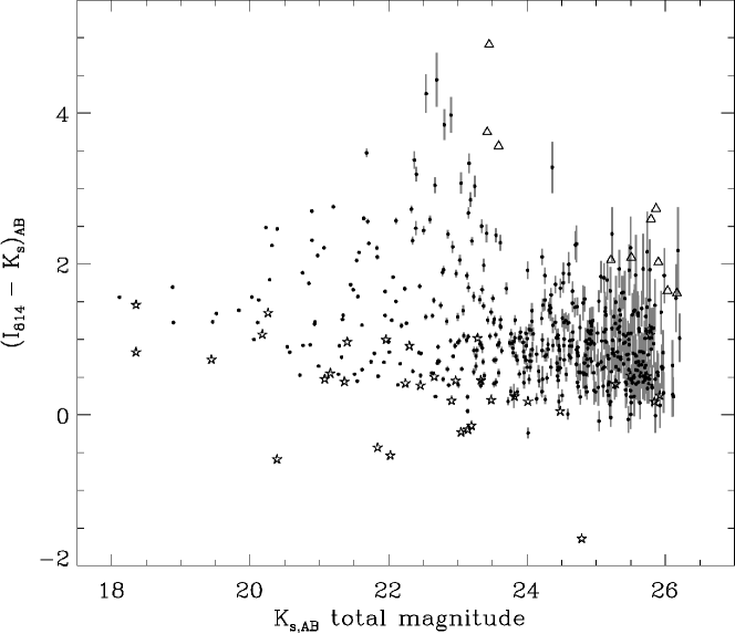
Figure 11: $I_{814}-K_{s}$ versus $K_{s}$ color-magnitude relation (on the AB system) for $K_{s}$-selected objects in the HDF-S. Only sources with a minimum of 20% of the total exposure time in all bands are included and identified stars are marked by a star symbol. Colors are plotted with $\pm 1\sigma$ error bars, and $I_{814}$ measurements with S/N $<2$ (triangles) are plotted at their $2\sigma$ confidence interval, indicating lower limits for the colors. There are more red sources with $I_{814}-K_{s}>2.6$ at $K\sim 23$ than at at $K\sim 24$ where the $I_{814}$ is still sufficiently deep to select them. The transformation of the $I_{814}-K_{s}$ color from the AB system to the Johnson magnitude system is $(I_{814}-K_{s})_{J}=(I_{814}-K_{s})_{AB}+1.43$.

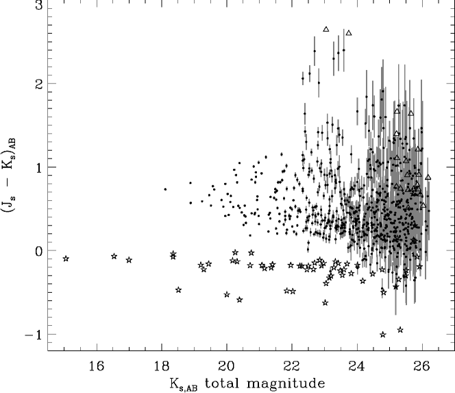
Figure 12: Same as Figure 11 for the $J_{s}-K_{s}$ color. Striking is the number the galaxies with very red NIR colors $J_{s}-K_{s}\gtrsim 1.34$ (on the AB system) or $J_{s}-K_{s}\gtrsim 2.3$ (Johnson). These systems have photometric redshifts $z>2$ and are extremely faint in the observer’s optical; as such they would not be selected with the U-dropout technique. Identified stars are well separated from redshifted galaxies and almost all have $J_{s}-K_{s}\leq 0$ colors. The transformation of the $J_{s}-K_{s}$ color from the AB system to the Johnson magnitude system is $(J_{s}-K_{s})_{J}=(J_{s}-K_{s})_{AB}+0.96$.

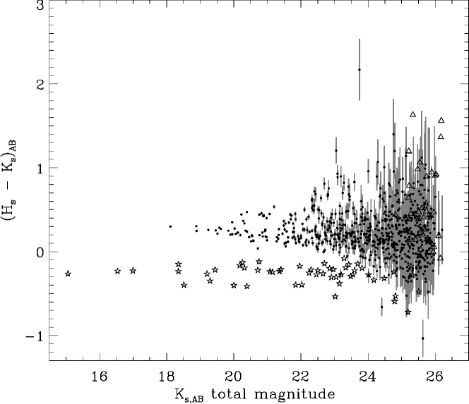
Figure 13: Same as Figure 11 for the $H-K_{s}$ color. One of the galaxies is extremely red with $H-K_{s}\approx 2.2$ and is barely visible in $J_{s}$ and $H$. The transformation of the $H-K_{s}$ color from the AB system to the Johnson magnitude system is $(H-K_{s})_{J}=(H-K_{s})_{AB}+0.48$.

8.2 Color-Magnitude Distributions

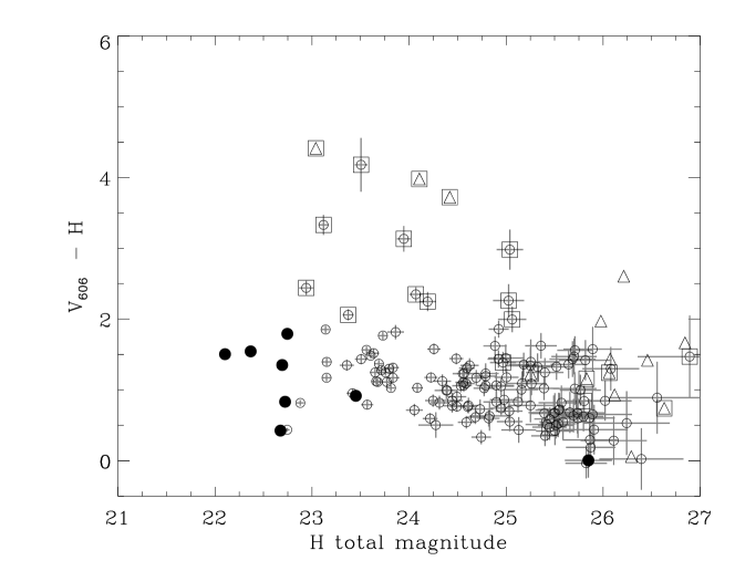
Figure 14: $V_{606}-H$ versus $H$ color-magnitude diagram (on the AB system) for galaxies in the HDF-S $K_{s}$-selected catalog with $1.95<z_{phot}<3.5$. Filled symbols indicate galaxies with spectroscopy. The number of candidates for red, evolved galaxies is much higher than in the HDF-N for a similar survey area, as shown in a identical plot in Fig. 1 of Papovich, Dickinson, & Ferguson (2001): we find 7 galaxies redder than $V_{606,AB}-H_{AB}\gtrsim 3$ and brighter than $H_{AB}\lesssim 25.5$, compared to only one in the HDF-N. Galaxies with S/N $<2$ for the $V_{606}$ measurement (triangles) are plotted at the $2\sigma$ confidence limit in $V_{606}$, indicating a lower limit on the $V_{606}-H$ color. The subsample of galaxies having red $(J_{s}-K_{s})_{J}>2.3$ colors (open squares) is also shown. The transformation of the $V_{606}-H_{s}$ color from the AB system to the Johnson magnitude system is $(V_{606}-H)_{J}=(V_{606}-H)_{AB}+1.26$.

Figures 11 – 14 show color-magnitude diagrams of $K_{s}$-selected galaxies in the HDF-S. The $I_{814}-K_{s}$ versus $K_{s}$ color-magnitude diagram in Figure 11 shows a large number of extremely red objects (EROs) with $I_{814}-K_{s}\gtrsim 2.6$ (on the AB system) or $(I_{814}-K_{s})_{J}\gtrsim 4$ (Johnson). There appears to be an excess of EROs at total magnitudes $K_{s,AB}\sim 23$ compared to magnitudes $K_{s,AB}\sim 24$. This is not caused by the insufficient signal-to-noise ratio in the $I_{814}$ measurements. In a similar diagram for the $J_{s}-K_{s}$ color shown in Figure 12, there is a striking presence at the same $K_{s}$ magnitudes of sources with very red $(J_{s}-K_{s})_{AB}\gtrsim 1.34$ or $(J_{s}-K_{s})_{J}\gtrsim 2.3$ colors. Such sources were also found by Saracco et al. (2001), using shallow NIR data, who suggested they might be dusty starbursts or ellipticals at $z>2$. Interestingly, any evolved galaxy with a prominent Balmer/4000Å discontinuity in their spectrum, like most present-day Hubble Type galaxies, would have such very red observed NIR colors if placed at redshifts $z>2$. While the $(J_{s}-K_{s})_{J}\gtrsim 2.3$ sources we find are generally morphologically compact, with exceptions, we do not expect the sources with good photometry to be faint cool L-dwarf stars because known colors of such stars are $(J_{s}-K_{s})_{J}\lesssim 2.1$ (see section 6.3). The photometric redshifts of all red NIR galaxies are $z_{phot}\gtrsim 2$, but they would be missed by ultraviolet-optical color selection techniques such as the U-dropout method, because most of them are barely detectable even in the deepest optical images. One bright NIR galaxy is completely undetected in the original WFPC2 images. The $(J_{s}-K_{s})_{J}\gtrsim 2.3$ sources are studied in more detail by Franx et al. (2002) and the relative contributions of these galaxies and U-dropouts to the rest-frame optical luminosity density will be presented in Rudnick et al. (2002b).

If we select sources with $1.95<z_{phot}<3.5$, we find clear differences in the $V_{606}-H$ versus $H$ color-magnitude diagram between our NIR-selected galaxies in the HDF-S and those of the HDF-N (compare Figure 14 to Figure 1 of Papovich, Dickinson, & Ferguson 2001). Over a similar survey area and to similar limiting depths, we find 7 galaxies redder than $(V_{606}-H)_{AB}\gtrsim 3$ and brighter than total magnitude $H_{AB}\lesssim 25.5$, compared to only one in the HDF-N.

Figure 15: The surface densities of galaxies selected by color in the 5$\sigma$ catalog of sources of HDF-S. Presented are galaxies with $(J_{s}-K_{s})_{J}>2.3$ (in Johnson magnitudes) (diamonds), extremely red objects with $(I_{814}-K_{s})_{J}>4$ (squares), and all $K_{s}$-selected galaxies (filled points) as a function total $K_{s}$-band AB magnitude. Only sources with a minimum exposure time of 40%, 40% and 90% of the total in $I_{814},J_{s}$ and $K_{s}$ are plotted, so that the selection in $K_{s}$ is uniform over the area, and the $I_{814}$ and $J_{s}$ observations are sufficiently deep to prevent a bias against objects with very red $I_{814}-K_{s}$ and $J_{s}-K_{s}$ colors. No corrections to the counts have been applied. The errorbars are poissonian and might underestimate the true uncertainty which would also contain contributions from large scale structure.

While the surface density of such galaxies is not well known, it is clear that the HDF-N contains far fewer of them than the HDF-S. It remains to be seen if this is just field-to-field variation, or that one of the two fields is atypical. The results of the second much larger FIRES field centered on MS1054-03 (Förster Schreiber et al., 2002) should provide more insight into this issue. We note that all 7 $(V_{606}-H)_{AB}\gtrsim 3$ galaxies in the HDF-S are also amongst the brightest 16 $(J_{s}-K_{s})_{J}>2.3$ sources. Figure 15 shows the surface densities of EROs and galaxies with $(J_{s}-K_{s})_{J}>2.3$ colors as function of $K_{s}$-band total magnitude. The surface density of EROs peaks around $K_{s,AB}\approx 23$ and then drops or flattens at fainter magnitudes, contrary to the number of $(J_{s}-K_{s})_{J}>2.3$ galaxies which keeps rising to the faintest $K_{s}$ total magnitudes in our catalog.

9 Summary and Conclusions

We have presented the results of the FIRES deep NIR imaging of the WFPC2-field of the HDF-S obtained with ISAAC at the VLT: the deepest ground-based NIR data available, and the deepest $K_{s}$-band of any field. We constructed a $K_{s}$-selected multicolor catalog of galaxies, consisting of 833 objects with $K_{s,AB}\lesssim 26$ and photometry in seven-bands from $0.3$ to $2.2\mu$ for 624 of them. These data are available electronically together with photometric redshifts for 567 galaxies. Our unique combination of deep optical space-based data from the HST together with deep ground-based NIR data from the VLT allows us to sample light redder than the rest-frame V-band in galaxies with $z\lesssim 3$ and to select galaxies from their rest-frame optical properties, obtaining a more complete census of the stellar mass in the high-redshift universe. We summarize our main findings below:

• The $K_{s}$-band galaxy counts in HDF-S turn over at the faintest magnitudes and flatten from $\alpha\approx 0.25$ at total AB magnitudes $22\lesssim K_{s}\lesssim 24$ to $\alpha\approx 0.15$ at $24\lesssim K_{s}\lesssim 26$; this is flatter than counts in previously published deep NIR surveys, where the FIRES HDF-S field is largest and deepest amongst these surveys. The nature of the scatter in the faint-end counts is yet unclear but field-to-field varations as well as different analysis techniques likely play a role.

• The HDF-S contains 7 sources redder than $(V_{606}-H)_{AB}\gtrsim 3$ and brighter than total magnitude $H_{AB}\lesssim 25.5$ at photometric redshifts $1.95<z_{phot}<3.5$, while such galaxies were virtually absent in the HDF-N. They are much redder than regular U-dropout galaxies in the same field and are candidates for relatively massive, evolved systems at high redshift. The difference with the HDF-N might just reflect field-to-field variance, calling for more observations to similar limits with full optical-to-infrared coverage. Results from the second and larger FIRES field centered on MS1054-03 (Förster Schreiber et al., 2002) should provide more insight into this issue.

• We find substantial numbers of red galaxies with $(J_{s}-K_{s})_{J}>2.3$ that have photometric redshifts $z_{phot}>2$. These galaxies would be missed by ultraviolet-optical color selection techniques such as the U-dropout method because most of them are barely detectable even in the deepest optical images. The surface densities of these sources in our field keeps rising down to the detection limit in $K_{s}$, in contrast to the number counts of EROs which peak at $K_{s,AB}\sim 23$ and then drop or flatten at fainter magnitudes.

The results of the HDF-S presented in this paper demonstrate the necessity of extending optical observations to near-IR wavelengths for a more complete census of the early universe. Our deep $K_{s}$-band data prove invaluable for they probe well into the rest-frame optical at $2<z<4$, where long-lived stars may dominate the light of galaxies. We are pursuing follow-up programs to obtain more spectroscopic redshifts needed to confirm the above results. Updates on the FIRES programme and access to the reduced images and catalogues can be found at our website http://www.strw.leidenuniv.nl/{̃}fires.

Table 1: Summary of the HDF-S Observations

Camera	Filter	Number of	Integration Time	Image Quality
		Exposures	(h)	(arcsec)
WFPC2	$F300W$	102	36.8	0$\farcs$16
WFPC2	$F450W$	51	28.3	0$\farcs$14
WFPC2	$F606W$	49	27.0	0$\farcs$13
WFPC2	$F814W$	56	31.2	0$\farcs$14
ISAAC	$J_{s}$	1007	33.6	0$\farcs$45
ISAAC	$H$	968	32.3	0$\farcs$48
ISAAC	$K_{s}$	2136	35.6	0$\farcs$46

Table 2: Zero Points for the HDF-S

	Zero Point
Data Set	Johnson mag	AB mag
$U_{300}$	19.43	20.77
$B_{450}$	22.01	21.93
$V_{606}$	22.90	23.02
$I_{814}$	21.66	22.09
$J_{s}$	24.70	25.60
$H$	24.60	25.98
$K_{s}$	24.12	25.98

Table 3: Background noise in the HDF-S images

Data Set	rms background variation	a	b	1$\sigma$ sky noise limit
$U_{300}$	1.34e-05	2.51	0.38	29.5
$B_{450}$	1.88e-05	2.65	0.40	30.3
$V_{606}$	3.80e-05	2.49	0.39	30.6
$I_{814}$	2.79e-05	2.59	0.39	30.0
$J_{s}$	0.0069	1.46	0.047	28.6
$H$	0.0165	1.43	0.044	28.1
$K_{s}$	0.0163	1.49	0.038	28.1

References

- Adelberger & Steidel (2000) Adelberger, K. L. & Steidel, C. C. 2000, ApJ, 544, 218
- Amico et al. (2001) P. Amico et al. eds, 2001, ISAAC-SW Data Reduction Guide (version 1.5)
- Barger et al. (2001) Barger, A. J., Cowie, L. L., Bautz, M. W., Brandt, W. N., Garmire, G. P., Hornschemeier, A. E., Ivison, R. J., & Owen, F. N. 2001, AJ, 122, 2177
- Bershady, Lowenthal, & Koo (1998) Bershady, M. A., Lowenthal, J. D., & Koo, D. C. 1998, ApJ, 505, 50
- Bertin & Arnouts (1996) Bertin, E. & Arnouts, S. 1996, A&AS, 117, 393
- Bessell & Brett (1988) Bessell, M. S. & Brett, J. M. 1988, PASP, 100, 1134 (JHKLMN photometric system)
- Bruzual & Charlot (2002) Bruzual A., G., & Charlot, S. 2001, in preparation
- Casertano et al. (2000) Casertano, S. et al. 2000, AJ, 120, 2747
- Cohen et al. (2000) Cohen, J. G., Hogg, D. W., Blandford, R., Cowie, L. L., Hu, E., Songaila, A., Shopbell, P., & Richberg, K. 2000, ApJ, 538, 29
- Coleman, Wu, & Weedman (1980) Coleman, G. D., Wu, C.-C., & Weedman, D. W. 1980, ApJS, 43, 393 (CWW80)
- Cowie et al. (2001) Cowie, L. L. et al. 2001, ApJ, 551, L9
- da Costa et al. (1998) da Costa, L et al. 1998 (astro-ph/9812105)
- Dickinson (2001a) Dickinson, M., 2001a, in preparation
- Dickinson et al. (2000) Dickinson, M. et al. 2000, ApJ, 531, 624
- Djorgovski et al. (1995) Djorgovski, S. et al. 1995, ApJ, 438, L13
- Fernández-Soto, Lanzetta, & Yahil (1999) Fernández-Soto, A., Lanzetta, K. M., & Yahil, A. 1999, ApJ, 513, 34 (FLY99)
- Förster Schreiber et al. (2002) Forster Schreiber, N.M. et al. 2002, in preparation
- Franx et al. (1989) Franx, M., Illingworth, G. D., Heckman, T. M., 1989, A.J., 98 538-576
- Franx et al. (2000) Franx, M. et al. 2000, The Messenger, 99, 20
- Franx et al. (2002) Franx, M. et al. 2002, in preparation
- Giavalisco, Steidel, & Macchetto (1996) Giavalisco, M., Steidel, C. C., & Macchetto, F. D. 1996, ApJ, 470, 189
- Giavalisco et al. (1998) Giavalisco, M., Steidel, C. C., Adelberger, K. L., Dickinson, M. E., Pettini, M., & Kellogg, M. 1998, ApJ, 503, 543
- Giavalisco & Dickinson (2001) Giavalisco, M. & Dickinson, M. 2001, ApJ, 550, 177
- Glazebrook & Bland-Hawthorn (2001) Glazebrook, K. & Bland-Hawthorn, J. 2001, PASP, 113, 197
- Guhathakurta, Tyson, & Majewski (1990) Guhathakurta, P., Tyson, J. A., & Majewski, S. R. 1990, ApJ, 357, L9
- Hauschildt et al. (1999) Hauschildt, P. H., Allard, F., Ferguson, J., Baron, E., & Alexander, D. R. 1999, ApJ, 525, 871
- Johnson (1966) Johnson, H. L. 1966, ARA&A, 4, 193
- Kauffmann & Charlot (1998) Kauffmann, G. & Charlot, S. 1998, MNRAS, 297, L23
- Kinney et al. (1996) Kinney, A. L., Calzetti, D., Bohlin, R. C., McQuade, K., Storchi-Bergmann, T., & Schmitt, H. R. 1996, ApJ, 467, 38
- Kirkpatrick et al. (2000) Kirkpatrick, J. D. et al. 2000, AJ, 120, 447
- Kron (1980) Kron, R. G. 1980, ApJS, 43, 305
- Lowenthal et al. (1997) Lowenthal, J. D. et al. 1997, ApJ, 481, 673
- Madau (1995) Madau, P. 1995, ApJ, 441, 18
- Maihara et al. (2001) Maihara, T. et al. 2001, PASJ, 53, 25
- Moorwood (1997) Moorwood, A. F. 1997, Proc. SPIE, 2871, 1146
- Moustakas et al. (1997) Moustakas, L. A., Davis, M., Graham, J. R., Silk, J., Peterson, B. A., & Yoshii, Y. 1997, ApJ, 475, 445
- Oke (1971) Oke, J. B. 1971, ApJ, 170, 193
- Papovich, Dickinson, & Ferguson (2001) Papovich, C., Dickinson, M., & Ferguson, H. C. 2001, ApJ, 559, 620 (P01)
- Persson et al. (1998) Persson et al. 1998 AJ, 116, 2475
- Pettini et al. (1998) Pettini, M., Kellogg, M., Steidel, C. C., Dickinson, M., Adelberger, K. L., & Giavalisco, M. 1998, ApJ, 508, 539
- Pettini et al. (2001) Pettini, M., Shapley, A. E., Steidel, C. C., Cuby, J., Dickinson, M., Moorwood, A. F. M., Adelberger, K. L., & Giavalisco, M. 2001, ApJ, 554, 981
- Pozzetti, Bruzual, & Zamorani (1996) Pozzetti, L., Bruzual A., G., & Zamorani, G. 1996, MNRAS, 281, 953
- Rudnick et al. (2001) Rudnick, G. et al. 2001, AJ, 122, 2205 (R01)
- Rudnick et al. (2002a) Rudnick, G. et al. 2002, in preparation (R02a)
- Rudnick et al. (2002b) Rudnick, G. et al. 2002, in preparation (R02b)
- Saracco et al. (2001) Saracco, P., Giallongo, E., Cristiani, S., D’Odorico, S., Fontana, A., Iovino, A., Poli, F., & Vanzella, E. 2001, A&A, 375, 1
- Sawicki & Yee (1998) Sawicki, M. & Yee, H. K. C. 1998, AJ, 115, 1329
- Shapley et al. (2001) Shapley, A. E., Steidel, C. C., Adelberger, K. L., Dickinson, M., Giavalisco, M., & Pettini, M. 2001, ApJ, 562, 95
- Schlegel, Finkbeiner, & Davis (1998) Schlegel, D. J., Finkbeiner, D. P., & Davis, M. 1998, ApJ, 500, 525
- Steidel et al. (1996a) Steidel, C. C., Giavalisco, M., Dickinson, M., & Adelberger, K. L. 1996, AJ, 112, 352
- Steidel et al. (1996b) Steidel, C. C., Giavalisco, M., Pettini, M., Dickinson, M., & Adelberger, K. L. 1996, ApJ, 462, L17
- Steidel, Pettini, & Hamilton (1995) Steidel, C. C., Pettini, M., & Hamilton, D. 1995, AJ, 110, 2519
- Steidel & Hamilton (1992) Steidel, C. C. & Hamilton, D. 1992, AJ, 104, 941
- Smail et al. (2000) Smail, I., Ivison, R. J., Owen, F. N., Blain, A. W., & Kneib, J.-P. 2000, ApJ, 528, 612
- Voit et al. (1997) Voit, M., ed. 1997, HST Data Handbook, Vol. 1 (version 3.1; Baltimore: STScI)
- Williams et al. (1996) Williams, R. E. et al. 1996, AJ, 112, 1335
- Williams et al. (2000) Williams, R. E. et al. 2000, AJ, 120, 2735