Improved Measurement of the Angular Power Spectrum of Temperature Anisotropy in the CMB from Two New Analyses of Boomerang Observations

Abstract

We report the most complete analysis to date of observations of the Cosmic Microwave Background (CMB) obtained during the 1998 flight of Boomerang. We use two quite different methods to determine the angular power spectrum of the CMB in 20 bands centered at $\ell=50$ to 1000, applying them to $\sim 50$% more data than has previously been analyzed. The power spectra produced by the two methods are in good agreement with each other, and constitute the most sensitive measurements to date over the range $300<\ell<1000$. The increased precision of the power spectrum yields more precise determinations of several cosmological parameters than previous analyses of Boomerang data. The results continue to support an inflationary paradigm for the origin of the universe, being well fit by a $\sim 13.5$ Gyr old, flat universe composed of approximately 5% baryonic matter, 30% cold dark matter, and 65% dark energy, with a spectral index of initial density perturbations $n_{s}\sim 1$.

1 Introduction

Measurements of anisotropies in the cosmic microwave background (CMB) radiation now tightly constrain the nature and composition of our universe. High signal-to-noise detections of primordial anisotropies have been made at angular scales ranging from the quadrupole (Bennett et al., 1996) to as small as several arcminutes (Mason et al., 2002; Pearson et al., 2002; Dawson et al., 2002). The power spectrum of temperature fluctuations shows a peak at spherical harmonic multipole $\ell\sim 200$ which has been detected with very high signal-to-noise by several teams (de Bernardis et al., 2000; Hanany et al., 2000; Halverson et al., 2001; Scott et al., 2002), and strong indications of peaks at higher $\ell$ have also been found (Halverson et al., 2001; Netterfield et al., 2002; de Bernardis et al., 2002).

Within the context of models with adiabatic initial perturbations, as are generally predicted by inflation, these measurements have been used in combination with various other cosmological constraints to estimate the values of many important cosmological parameters. Combining their CMB data with weak cosmological constraints such as a very loose prior on the Hubble constant, various teams have made robust determinations of several parameters, including the total energy density of the universe $\Omega_{total}$, the density of baryons $\Omega_{b}$, and the value of the density perturbation power spectral index, $n_{s}$  (Lange et al., 2001; Balbi et al., 2000; Pryke et al., 2001; Netterfield et al., 2002). Many other parameters are tightly constrained when stronger constraints on cosmology are assumed.

We report here new results from the 1998 Antarctic flight of the Boomerang experiment. Previous results from this flight using less data than included here were published in de Bernardis et al. (2000) (hereafter B00) and Netterfield et al. (2002) (hereafter B02). Here we use the two very different analysis methods of B00 and B02, and apply them over a larger fraction of the dataset to make an improved measurement of the CMB angular power spectrum.

2 Instrument and Observations

Boomerang is a balloon-borne instrument, designed to measure the anisotropies of the CMB at sub-degree angular scales. The instrument consists of a bolometric mm-wave receiver mounted at the focus of an off-axis telescope, borne aloft on an altitude-azimuth pointed balloon gondola. Details of the instrument as it was configured for the 1998 Antarctic flight, and its performance during that flight, are given in Crill et al. (2002).

The receiver consists of 16 bolometers, optically coupled to the telescope through a variety of cryogenic filters, feedhorns, and reimaging optics. We report here results from four of the six 150 GHz detectors in the focal plane, the same four analyzed in B02. The other two 150 GHz detectors exhibited non-stationary noise properties and are not used in the analysis.

The telescope has a 1.2 m diameter primary mirror and two cryogenic reimaging mirrors mounted to the 2K surface of the receiver cryostat. These optics produce ($9.2^{\prime}$,$9.7^{\prime}$,$9.4^{\prime}$,$9.5^{\prime}$) FWHM beams at 150 GHz in the four channels used here. The measured beams are nearly symmetric Gaussians; the beamshapes are estimated by a physical optics calculation, and calibrated by measurements on the ground prior to flight. Uncertainty in the pointing solution ($2.5^{\prime}$ rms) is estimated to smear the resolution of these physical beams to an effective resolution of ($10.9^{\prime}$,$11.4^{\prime}$,$11.1^{\prime}$,$11.2^{\prime}$) FWHM respectively. Based on the scatter of our various beam measures, and combined with our uncertainty in the smearing due to the pointing solution errors, we assign a 1-$\sigma$ uncertainty in the FWHM beamwidth of $1.4^{\prime}$ in all channels. This introduces an uncertainty in the measured amplitude of the power spectrum that grows exponentially with $\ell$ and that is correlated between all bands. This effect reaches a maximum of $\pm 40$% in our highest bin ($\ell=1000$), and is illustrated in Figure 2 of B02.

The payload was launched from McMurdo Station, Antarctica on 29 December 1998 and circumnavigated the continent in 10.5 days at an approximately constant latitude of -78 degrees. During the flight, 247 hours of data were taken, most of them on a “CMB region” that was chosen for its very low dust contrast seen in the IRAS $100\mu$ maps of this region (Moshir et al., 1992).

The field observed in CMB scan mode is shown in Figure 1. We analyze a subset of this sky coverage here, chosen to be a contiguous region that is both sufficiently far from the galactic plane and well-covered by our observations. Figure 1 shows the boundary of the region that we analyze in this paper. This region covers 2.94% of the sky, and is defined as the intersection of:

• an ellipse centered on RA = $88^{\circ}$, $\delta=-47^{\circ}$, with semiaxes $a=25^{\circ}$ and $b=19^{\circ}$, where the short axis lies along the local celestial meridian,

• the strip bounded by $-59^{\circ}<\delta<-29.5^{\circ}$,

• and the region with galactic latitude $b<-10^{\circ}$.

This contour includes the best observed area of the survey, while remaining far enough from the galactic disk to minimize galactic dust contamination. It also does not have any small scale features (such as sharp corners) that could induce excessive ringing in the power spectrum extracted using one of our two methods (FASTER) discussed below. This contour also excludes most of the scan turnarounds, where the scan speed is reduced and the low frequency noise can contaminate the angular scales of interest.

The vast majority of our observations of this region were made by fixing the elevation of the telescope and scanning azimuthally by $\pm 30^{\circ}$, typically centered roughly $30^{\circ}$ from the anti-solar azimuth. Also used were the “CMB region” portions of infrequently made ($\sim 1$ per hour) wider scans designed to traverse the Galactic plane as well.

CMB observations were made by scanning at three elevations ($45^{\circ}$, $50^{\circ}$ and $55^{\circ}$), and at two azimuthal scan speeds (1 degree/second and 2 degrees/second, hereafter 1dps and 2dps respectively). The rising, setting and rotation of the sky observed from $-78^{\circ}$ latitude causes these fixed elevation scans to fill out the coverage of a two dimensional map. The color coding in our sky coverage map (Figure 1) gives the errors per pixel after coadding the data from the four 150 GHz detectors.

The raw detector timestreams are cleaned, filtered and calibrated before being fed to the mapping and power spectrum estimation pipelines described below. The cleaning and filtering used in this analysis is identical to that described in B02 and is also described in Crill et al. (2002); we give the most relevant details here.

Bolometers are sensitive to any input that changes the detector temperature, including cosmic ray interactions in the detector itself, radiofrequency interference (RFI), and thermal fluctuations of the baseplate heatsink temperature. After deconvolving the raw bolometer data with the filter response of the detector and associated electronics, RFI, cosmic rays, and thermal events are found by a variety of pattern-matching and map-based iterative techniques. Bad data are then flagged and replaced by a constrained realization of the noise so that nearby data can be used. In the four channels used here, approximately 4.8% is flagged. The tails of thermal events are fit to an exponential and corrected, and the data are used in the subsequent analysis. Finally, a very low frequency high-pass filter is applied in the Fourier domain, with a transfer function $F(f)=0.5(1-\cos(\pi f/0.01\mbox{Hz}))$ for $f\leq 0.01$ Hz, $F(f)=1$ for $f>0.01$ Hz.

Figure 1: The sky covered by CMB observations; the color scale indicates the depth of coverage (diagonal component of the noise covariance matrix) in a $7^{\prime}$ Healpix pixel, in the map produced by the MADCAP analysis described below. The region enclosed by the solid line is that used for the power spectrum estimation. The three circles show the locations of three bright known quasars; data within a $0.5^{\circ}$ radius of the quasars is not used in the power spectrum estimation.

3 Data Analysis Methods

This paper reports our third analysis of data from the 1998 flight. In B00 we reported the angular power spectrum found by analyzing data from a single detector covering 1.0% of the sky, using roughly one detector-day of integration. In B02 we reported results from four 150 GHz detectors, using 17 detector-days of integration on 1.9% of the sky. Here we report new results using 50% more data from those same four detectors, using over 24 detector-days of integration on 2.9% of the celestial sphere.

The results reported here use the same timestream cleaning and pointing solutions described in B02. In addition to the larger sky cut, here we use two independent and very different analysis methods which derive the angular power spectrum of the CMB from those timestream inputs. One, using the MADCAP CMB analysis software suite (Borrill, 1999), creates a maximum likelihood map and pixel-pixel covariance matrix from the input detector timestreams and measured detector noise properties. The power spectrum is derived from the map and its covariance matrix; this was the method used in B00. The other method, based on the MASTER/FASTER algorithms described in Hivon et al. (2002) and Contaldi et al. (2002), relies on a spherical harmonic transform of a filtered, simply binned map created from those timestreams; the angular power spectrum in the filtered map is related to the full-sky unfiltered angular power spectrum through corrections derived from Monte-Carlos of the input detector timestream and model CMB sky signals. In the FASTER procedure, the best fit angular power spectrum is then obtained by using an iterative quadratic estimator analogous to that used in conventional maximum likelihood procedures. This method was used in B02.

A theme of this paper is the comparison of the results from these two very different analysis paths, and the stability of the cosmological results to any differences in the derived power spectra.

3.1 Detector noise estimation

Both MADCAP and FASTER require an accurate estimate of the detector noise properties in order to determine the angular power spectrum. We estimate these noise properties from the data themselves, using an iterative method to create an optimal, maximum likelihood map of the sky signal. We then remove this signal from the detector timestream prior to calculating the noise statistics. This method is described in both B02 and Prunet et al. (2001).

For bolometer $i$ and iteration $j$, ${\bf d}_{i},{\bf A}_{i}$, ${\bf n}_{i}^{(j)}$, ${\bf N}_{i}^{(j)}$, and ${\bf\Delta}^{(j)}$ are respectively the data, pointing matrix, noise timestream, noise timestream correlation matrix, and sky map. The sky map and noise timestream correlation matrices are found by iteration:

1. Given the data timestream and estimated map, solve for the noise-only timestream with ${\bf n}^{(j)}_{i}={\bf d}_{i}-{\bf A}_{i}{\bf\Delta}^{(j)}$

2. Use ${\bf n}^{(j)}_{i}$ to construct the noise timestream correlation matrix, ${\bf N}_{i}^{(j)}=\langle{\bf n}_{i}^{(j)}{\bf n}_{i}^{(j)\dagger}\rangle$

3. Solve for a new version of the map using ${\bf\Delta}^{(j+1)}=(\sum\limits_{i}{\bf A}_{i}^{\dagger}{\bf N}_{i}^{(j)-1}{\bf A}_{i})^{-1}\sum\limits_{i}{\bf A}_{i}^{\dagger}{\bf N}_{i}^{(j)-1}{\bf d}_{i}$

4. Return to step 1, using the new version of the map, and repeat. Iterate until the map ${\bf\Delta}$ and the noise correlation matrices ${\bf N}_{i}$ are stable.

For stationary noise ${\bf N}_{i}$ is diagonal in Fourier space, with the diagonal elements equal to the power spectrum of the noise. We also assume, and check in practice, that the noise correlation between channels is negligible.

The noise correlation matrix ${\bf N}_{i}$ is computed in Fourier space from the noise timestream ${\bf n}_{i}$ with a simple periodogram estimator. The maximum likelihood map of the combined bolometers, ${\bf\Delta}$, is computed using a conjugate gradient approach (Doré et al., 2001), which improves the recovery of large scale modes in the map.

Solving for all channels in a combined way takes advantage of the redundant observations of the sky, therefore offering the best possible separation between signal and noise in the time streams for each bolometer. The noise power spectrum estimation is well-converged after a few iterations, typically three or four.

In this iterative procedure, we find a single maximum-likelihood map using all the data from all detectors. In practice a separate noise covariance is solved for in each of the 78 contiguous data “chunks”, bordered by elevations moves or other timestream disturbances. Thus, very slowly varying noise properties (eg a drift in the instrument noise) will not affect the analysis. Additionally, a line is evident in the noise power spectrum of the timestream data, varying slowly between 8 and 9 Hz over the course of the flight. We remove the effects of this non-stationary source of noise by removing information in the timestream between 8 and 9 Hz. These frequencies correspond to angular scales $\ell>1000$, outside the range that we report here, for all scan speeds.

3.2 The MADCAP Analysis Path

Given a pixel-pointed time-ordered dataset $\bf d$ with piecewise stationary Gaussian random noise, the maximum likelihood pixel map ${\bf\Delta}$ and pixel-pixel noise correlation matrix ${\bf C}_{N}$ are (Wright, 1996; Tegmark, 1997; Ferreira & Jaffe, 2000)

$${\bf\Delta} = ({\bf A}^{\dagger}{\bf N}^{-1}{\bf A})^{-1}{\bf A}^{\dagger}{\bf N}^{-1}{\bf d}$$

$${\bf C}_{N} = ({\bf A}^{\dagger}{\bf N}^{-1}{\bf A})^{-1}$$ (1)

where, as before, ${\bf A}$ is the pointing matrix and ${\bf N}$ is the block-Toeplitz time-time noise correlation matrix.

Assuming that the CMB signal is Gaussian and azimuthally symmetric, the maximum likelihood angular power spectrum $C_{l}$ is that which maximizes the log-likelihood of the derived map given that spectrum (Gorski, 1994; Bond et al., 1998),

$${\cal L}({\bf d}|C_{\ell})=-\frac{1}{2}\left({\bf d}^{\dagger}\,{\bf C}^{-1}\,{\bf d}-{\rm Tr}\left[\ln{\bf C}\right]\right),$$ (2)

where ${\bf C}$ is the full pixel-pixel covariance matrix. The CMB signal and the detector noise are uncorrelated, so ${\bf C}$ is just the sum of the ${\bf C}_{N}$ found above, and the theory pixel-pixel covariance matrix ${\bf C}_{T}$ derived for a particular set of $C_{\ell}$’s.

In the MADCAP analysis path (Borrill, 1999) we solve these equations exactly, calculating the closed form solution for the map, using quasi Newton-Raphson iteration to find the set of $C_{\ell}$’s that maximizes the log-likelihood (Bond et al., 1998). Because the pixel-pixel correlation matrices are dense, the operation count scales as the cube, and the memory requirement as the square, of the number of pixels in the map. This imposes serious practical constraints on the size of the problems we can tackle; by optimizing our algorithms to minimize the scaling prefactors, and using massively parallel computers, we have been able to solve systems with up to O($10^{5}$) pixels - sufficient to analyze this dataset at $7^{\prime}$ pixelization.

There are two analyses that we want to perform on this dataset, each of which involve both map-making and power-spectrum estimation. First, we want to analyze the full dataset including all four channels at both scan speeds, to solve for the CMB angular power spectrum. Second, we want to perform a systematic test of the self-consistency of the data, differencing two halves of the data and checking that the sky signal disappears.

For the first of these, we construct a time-ordered dataset by concatenating the data from all four channels at both scan speeds, and solve for the map using the eight associated time-time noise correlation functions. This timestream consists of 163,726,965 observations of 160,805 pixels. Using 400 processors on NERSC’s 3000-processor IBM SP3, the associated map and pixel-pixel noise correlation matrix can be calculated from equation 1 in about 4 hours. Pixels not included in the cut being analyzed here are removed from the map, and the corresponding rows and columns of the pixel-pixel noise correlation matrix are excised, equivalent to marginalizing over them. The resulting map contains 92251 pixels, and the associated noise correlation matrix fills 70 Gb of memory at 8-byte precision.

For the second analysis, we construct two time-ordered datasets, each containing the data from all four channels but at only one of the two scan speeds. The 2dps time-ordered data contains 74,879,196 observations over 124,257 pixels, while at 1dps we have 88,832,768 observations over 151,654 pixels. Having made the maps and pixel-pixel noise correlation matrices from each timestream we apply our cut as above, and in addition remove any pixels within the cut that are not observed in both halves of the flight. This results in two maps (${\bf\Delta_{A}}$ and ${\bf\Delta_{B}}$) and their associated noise correlation matrices each covering an identical subset of 88,407 pixels. We then extract the power spectrum of the map ${\bf\Delta}_{J}=({\bf\Delta}_{A}-{\bf\Delta}_{B})/2$, taking the noise correlation matrix of ${\bf\Delta}_{J}$ to be the appropriately weighted sum of those for the component maps, ${\bf C}_{N}^{J}=({\bf C}_{N}^{A}+{\bf C}_{N}^{B})/4$. This assumes the 2dps and 1dps noise are uncorrelated. In the power spectrum estimation process we assume a CMB-like theory correlation matrix when calculating the $C_{\ell}$’s.

The finite extent of our maps creates finite correlation between our estimates of the power in nearby multipoles. However, we can reduce these correlations to small levels by calculating the power in tophat bins of sufficient width. We choose bins of width $\Delta\ell=50$, centered on $\ell=50,100,150,...1000$, together with additional “junk” bins below $\ell=25$ and above $\ell=1025$, which are included to prevent very low-$\ell$ and very high-$\ell$ power from being aliased into the range of interest. This binning reduces the correlations between adjacent bins to to less than $\sim 13$% between neighboring bands.

The power in a multipole bin is related to the power in the individual multipoles in that bin through a shape function: $C_{\ell}=C_{b}C_{\ell}^{shape}$. Although we are free to choose any spectral shape within each bin, experience shows that for relatively narrow bins the particular choice makes very little difference. We can explicitly account for the assumed spectral shape in our cosmological parameter extraction; here we use a flat shape function such that $\ell(\ell+1)C_{\ell}^{shape}={\rm constant}$.

The maps derived from the time-ordered data have been smoothed by both the detector beams and the common pixelization. For constant, circularly symmetric beams and pixels we can account for this exactly by incorporating the appropriate multipole window function in the pixel-pixel signal correlation matrix, ${\bf C}_{T}$.

The fact that each detector has a different beam means that ideally we should construct individual maps and noise correlation matrices for each channel and solve for the maximum likelihood power spectrum of all four maps (each convolved with its own beam) simultaneously. However, this would give a 4-fold increase in the number of pixels, and a 64-fold increase in the compute time. Instead, we analyze the single all-channel map assuming a noise-weighted average beam; this approximation is quantitatively justified by tests done with the FASTER pipeline, below.

We use the HEALPIX pixelization (Górski et al., 1998); in this scheme, the pixels have equal area but are asymmetric and have varying shapes. These slightly different shapes lead to pixel-specific window functions. Calculating all of the individual pixel window functions at our resolution is not feasible; instead, we use the all-sky average HEALPIX window function appropriate for our resolution.

By comparing individual pixel window functions at lower resolution, we can set an upper limit on the errors that may be induced by this approximation. Scaling to $27^{\prime}$ pixels (a factor of 4 larger) we find maximum deviations of 5% in temperature (ie, 10% in power) in the ratio of actual pixel window functions to the average pixel window function on the whole celestial sphere, at the correspondingly scaled $\ell$ of 1024/4 = 256. Thus, the pixel window function employed cannot be more than 5% (corresponding to an error in $C_{\ell}$ of 10%) off the true value at our highest $\ell$. In fact, since the field incorporates pixels of many geometries, averaging will make the error much smaller, realistically less than 1% in temperature.

Thus far we have assumed that the time-ordered data is comprised of CMB signal and stationary Gaussian noise only. However, we know that in our data there are systematics that lead to residual constant-declination stripes in the map. Failure to account for these residuals leads to the detection of a signal in the (1dps-2dps)/2 difference maps, which should be pure noise maps. In the MADCAP approach we account for these residuals by marginalizing over the contaminated modes when deriving the power spectrum from the map (Borrill et al., 2002). Specifically, to give zero weight to a particular pixel-template we add infinite noise in that mode to the pixel-pixel correlation matrix

$${\bf C}^{-1}\rightarrow lim_{\sigma\rightarrow\infty}\left({\bf C}+\sigma^{2}{\bf M}^{\dagger}{\bf M}\right)^{-1}$$ (3)

where ${\bf M}$ is the matrix of orthogonal templates, one of each mode to be marginalized over. Applying the Sherman-Morrison-Woodbury formula this reduces to

$${\bf C}^{-1}\rightarrow{\bf C}^{-1}-{\bf C}^{-1}{\bf M}\left({\bf M}^{\dagger}{\bf C}^{-1}{\bf M}\right)^{-1}{\bf M}^{\dagger}{\bf C}^{-1},$$ (4)

yielding a readily calculable correction - requiring computationally inexpensive matrix-vector operations only – to the inverse correlation matrix. Now whenever we multiply by ${\bf C}^{-1}$ in estimating the power spectrum we simply add the appropriate correction term. For the residual constant-declination stripes in this dataset we construct a sine and cosine template along each line of pixels of constant declination for all modes with wavelengths longer than 32 pixels (about 4 degrees).

Once the iterative power spectrum estimation has converged, the error bars on each bin are estimated from the initial (zero signal) and final bin-bin Fisher information matrices using the offset lognormal approximation (Bond et al., 1998).

3.3 The FASTER Analysis Path

The FASTER pipeline is based on the MASTER technique described in Hivon et al. (2002). MASTER allows fast and accurate determination of $C_{\ell}$ without performing the time consuming matrix-matrix manipulations that characterize exact methods such as MADCAP (Borrill, 1999).

As in MADCAP, there are two separate steps in the FASTER path; mapmaking, and power spectrum estimation from that map. In our current implementation of FASTER, we make a map from the data by naively binning the timestream into pixels on the sky. To reduce the effects of $1/f$ noise on this naively binned map, a brick-wall highpass Fourier filter is first applied to the timestream at a frequency of 0.1 Hz for the 1dps data, and 0.2 Hz for the 2dps data.

The spherical harmonic transform of this naively binned map is calculated using a fast ${\cal O}(N_{pix}^{1/2}\ell)$ method based on the Healpix tessellation of the sphere (Górski et al., 1998). The angular power in a noisy map, $\tilde{C_{\ell}}$, can be related to the true angular power spectrum on the full sky, $C_{\ell}$, by the effect of finite sky coverage ($M_{\ell\ell^{\prime}}$), time and spatial filtering of the maps ($F_{\ell}$), the finite beam size of the instrument ($B_{\ell}$), and instrument noise (${N_{\ell}}$) as

$$\left\langle\widetilde{C_{\ell}}\right\rangle=\sum_{\ell^{\prime}}M_{\ell\ell^{\prime}}F_{\ell^{\prime}}B_{\ell^{\prime}}^{2}\left\langle C_{\ell^{\prime}}\right\rangle+\left\langle\widetilde{N_{\ell}}\right\rangle.$$ (5)

The coupling matrix $M_{\ell\ell^{\prime}}$ is computed analytically. $B_{\ell}$ is determined by the measured beam and the pixel window function assuming here that the pixel has a circular symmetry. $F_{\ell}$ is determined from Monte-Carlo simulations of signal-only time streams, and $N_{\ell}$ from noise-only simulations of the time streams.

The simulated time streams are created using the actual flight pointing and transient flagging. The signal component of these time streams is generated from simulated CMB maps, while the noise component is from realizations of the measured detector noise $n(f)$. In both cases the same high pass filtering (0.1 Hz at 1dps and 0.2 Hz at 2dps) and notch filtering (between 8 and 9 Hz, to eliminate the previously mentioned non-stationary spectral line in the timestream data) is applied to the simulated TOD as to the real one. $F_{\ell}$ and $N_{\ell}$ are determined by averaging over 600 and 750 realizations respectively. Once all of these components are known the power spectrum estimation is carried out as follows.

A suitable quadratic estimator of the full sky spectrum in the cut sky variables ${\tilde{C}}_{\ell}$ together with its Fisher matrix is constructed via the coupling matrix $M_{\ell\ell^{\prime}}$ and the transfer function $F_{\ell}$ (Bond et al., 1998; Netterfield et al., 2002). The underlying power is recovered through the iterative convergence of the quadratic estimator onto the maximum likelihood value as in standard maximum likelihood techniques. A great simplification and speed-up is obtained due to the diagonality of all the quantities involved, effectively avoiding the ${\cal O}(N^{3})$ large matrix inversion problem of the general maximum likelihood method. The extension of the quadratic estimator formalism to Monte-Carlo techniques such as MASTER have the added advantage that the Fisher matrix characterizing the uncertainty in the estimator is recovered directly in the iterative solution and does not rely on any potentially biased signal+noise simulation ensembles. A detailed discussion of the FASTER extension to the MASTER procedure can be found in Contaldi et al. (2002).

A drawback of using naively binned maps in the pipeline is that the aggressive time filtering completely suppresses the power in the maps below a critical scale $\ell_{c}\approx 50$ (Hivon et al., 2002). This results in one or more bands in the power spectrum running over modes with no power and which are thus unconstrainable. In practice we deal with this by binning the power so that many of the degenerate modes lie within the first band $2<\ell\leq 25$. The power in the degenerate band can then be regularized to zero power or a level consistent with the DMR large scale results. Regularizing with a non-zero value carries the disadvantage that the second band $25<\ell\leq 75$ will be non-trivially correlated with power which carries a theoretical bias. Regularizing with zero power results in no correlations between the first two bands and is more consistent with the filtering done on the Monte-Carlo maps which sets the signal in the affected modes to zero identically below $\ell_{c}$. We adopt the latter approach in this analysis to recover a useful band which we label as $25<\ell\leq 75$. However, as the window functions will show below (Figure 12), most of the information in this band comes from $50<\ell\leq 75$.

The FASTER pipeline allows the use of non-uniform masks applied to the observed patch of sky. We have experimented with a number of such weighting schemes for our patch including total variance weighting $1/(S+N)$ and Weiner-like $S/(S+N)$ weighting where $S$ is the Monte-Carlo estimated variance of the coadded signal in the pixel (which varies from pixel to pixel because of the high pass filtering applied to the time data stream and the non-uniform scanning speed) and $N$ is the variance of the noise in the pixel. We have found the $1/(S+N)$ weighting gives optimal results for this particular patch and coverage scheme of this analysis.

In order to remove any effect of the constant-declination striping contaminant described above a further (spatial) filtering step is applied to all the maps in the pipeline. The HEALPIX map is projected to a rectangular, square-pixel map, where a spatial Fourier filter is applied that removes all modes in the map with wavelengths greater than 8.2 degrees in the RA direction. This filtered map is then projected back to the HEALPIX pixelization.

The inclusion of several channels is achieved by averaging the maps (both from the data, and from the Monte-Carlos of each channel) before power spectrum estimation. Weighting in the addition is by hits per pixel, and by receiver noise at 1Hz. Each channel has a slightly different beam size, which is taken into account in the generation of the simulated maps. The Monte-Carlo procedure employed in FASTER and MASTER ensures that the estimated power is explicitly unbiased with respect to any known systematics, thus any inaccuracy in assuming a common $B_{\ell}$ in the angular power spectrum estimation is then absorbed into $F_{\ell}$. Similarly, any inaccuracy on the effective pixel window function for the patch of sky under consideration would be absorbed into $F_{\ell}$.

The calculation of the full angular power spectrum and covariance matrix for the four good 150 GHz channels of Boomerang ($\sim 350,000$ $3.5^{\prime}$ pixels and $\approx 216,000,000$ time samples; this is different from the MADCAP numbers given above because non-CMB sections of the timestream are treated differently) takes approximately four hours running on six nodes of the NERSC IBM SP3.

3.4 Application to Data

When treating real data, each of the methods described has particular advantages. MADCAP is an “optimal” tool, in the sense that it uses the full statistical power of the data in deriving the power spectrum; no other method can use the same data and produce a power spectrum with smaller errorbars. In addition, it produces a maximum-likelihood map and pixel-pixel covariance matrix that take advantage of the full cross-linking of the scan strategy. However, the MADCAP algorithms are computationally very costly. This leads to the use of several approximations (eg the use of a single beam for the four channels, using an average pixel window function, and fitting errors as a lognormal function), and reduces our ability to use this method for wide-ranging testing of potential systematic effects. With our current computing power and sky cut, we are limited to a $7^{\prime}$ pixelization with MADCAP.

The FASTER method provides a less-optimal estimate of the power spectrum, but is computationally much more rapid. As will be shown below, in our case the FASTER results are nearly as statistically powerful as those from MADCAP. The rapid computational turnaround allows the use of finer pixelization ($3.5^{\prime}$), and extensive systematic testing and modeling of potential systematic errors. Additionally, FASTER is capable of handling independent beams, and enables the computation of a true window function for our $\ell$ bins for use in parameter extraction.

4 Signal maps

The first step in each pipeline is the production of a sky map. The fundamental differences between the two analysis paths are well illustrated by a visual comparison of the two maps, shown in Figure 2. Though there is a high correlation of the small-scale structure in these two maps, their overall appearance is strikingly different, due primarily to the time-domain filtering that suppresses large scale structure in the FASTER map. In addition, the FASTER map has had the constant declination modes removed (hereafter, “destriped”), while the MADCAP map has not. (The MADCAP destriping occurs via marginalization over contaminated modes during the power spectrum estimation). The MADCAP map should be interpreted in concert with its covariance matrix, which describes which modes in the map are well constrained and which are not. The FASTER procedure does not create a covariance matrix; the correlations in the map are accounted for in the Monte-Carlo process. Thus while it is reassuring that the two maps show similar structure on small scales, a quantitative comparison can only be made by proceeding through the estimation of the angular power spectrum with each method.

Figure 2: The maps of CMB temperature produced by MADCAP (top) and FASTER (bottom). For comparison, both maps are pixelized at $7^{\prime}$; in practice we use a $7^{\prime}$ ($3.5^{\prime}$) pixelization in the MADCAP (FASTER) analysis. The strikingly different appearance of the maps, with the MADCAP map preserving more information on large scales, illustrates some of the significant differences in the two analysis methods, as described in the text.

5 FASTER Analysis consistency tests

The MADCAP analysis is limited to $7^{\prime}$ pixelization, and assumes a common beam window function for the four channels. We have used the FASTER pipeline to check the effect of this coarser pixelization and window function assumption with respect to the baseline FASTER result, which is calculated using $3.5^{\prime}$ pixels and individual window functions for each channel. The baseline FASTER result is shown in Figure 3, which also gives results derived using $7^{\prime}$ pixels, and results derived using the same “single beam” assumption used by MADCAP. As can be seen in the figure, the single beam approximation has negligible effect. The $7^{\prime}$ pixelization does have some effect, but it is small compared with the statistical errors.

Figure 3: Angular power spectra derived from the FASTER pipeline. The solid black circles in each panel show the reference FASTER spectrum, which is derived from a $3.5^{\prime}$ pixelized map using S+N weighting, spatially filtered as described in the text to remove constant-declination stripes. In the top panel the reference spectrum is compared with a spectrum derived using a single beam window function, as in MADCAP. The second panel shows the effect of using $7^{\prime}$ pixelization. The third panel illustrates the effect of removing the constant declination stripes; the primary effect is to increase the error in the first bin. The bottom panel shows the result of using a uniformly weighted map and neglecting to remove the constant declination stripes. The top three panels show excellent agreement with the reference spectrum, while the bottom panel shows good agreement except at very high $\ell$.

We have also tested the robustness of the FASTER result to other changes in the pipeline. Figure 3 also shows the effects of destriping, and of using signal+noise weighting (rather than uniform weighting). These have some affect on the power spectrum, again smaller than the statistical errors. Note that we expect these to have some effect given that the information content of the map is modified by these procedures.

Another test of the robustness of the angular power spectrum is to change the details of the $\ell$ binning. We have used the FASTER pipeline to derive power spectra with $\Delta\ell=40$ bins, and for $\Delta\ell=50$ bins shifted by 25 from our fiducial binning. Both of these give excellent agreement with power spectrum of Figure 3.

6 Internal Consistency Tests

The analysis pipelines described above deliver an estimated CMB power spectrum along with statistical errors on that power spectrum. Below, we will show the CMB power spectra derived from the maps, and use those results to estimate cosmological parameters. Before doing so, we describe here a variety of internal consistency tests designed to check for residual systematic contamination.

Our internal consistency checks are done by splitting the dataset roughly in half, making a map with each half of the data, subtracting these two maps, and asking whether the power spectrum of the residual map is consistent with pure detector noise. Note that one only expects the two maps to be identical if they contain the same information; if the two maps have been observed or filtered differently, perfect agreement is not expected.

Our most powerful internal consistency check is to take data that was gathered while scanning the gondola azimuthally at 1dps (roughly the first half of the flight) and compare it with data taken during 2dps scans (roughly the second half of the flight). This tests for effects that vary over long timescales, position of the gondola over the Earth, position of the scan region with respect to the Sun, and instrumental effects that are modulated by scan speed. The latter include any mis-estimate of the transfer function of the detector system and any non-stationary noise in the detector system. Hereafter, this test is referred to as the (1dps-2dps)/2 consistency test. Each pipeline was used to produce and estimate the power spectrum of a (1dps-2dps)/2 map.

Figure 4 shows MADCAP and FASTER (1dps-2dps) difference maps, each pixelized at $7^{\prime}$. Many of the gross features apparent in both maps are due to the variations in S/N, as can be seen by comparison with Figure 1. The MADCAP map is not destriped, because the destriping in that pipeline is done with a constraint matrix in deriving the power spectrum. The FASTER map is destriped; and appears significantly cleaner to the eye. In practice, a $3.5^{\prime}$ pixelized map is used in the FASTER analysis; here we display a $7^{\prime}$ map so the noise level per pixel remains comparable to the MADCAP version.

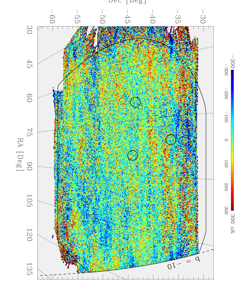
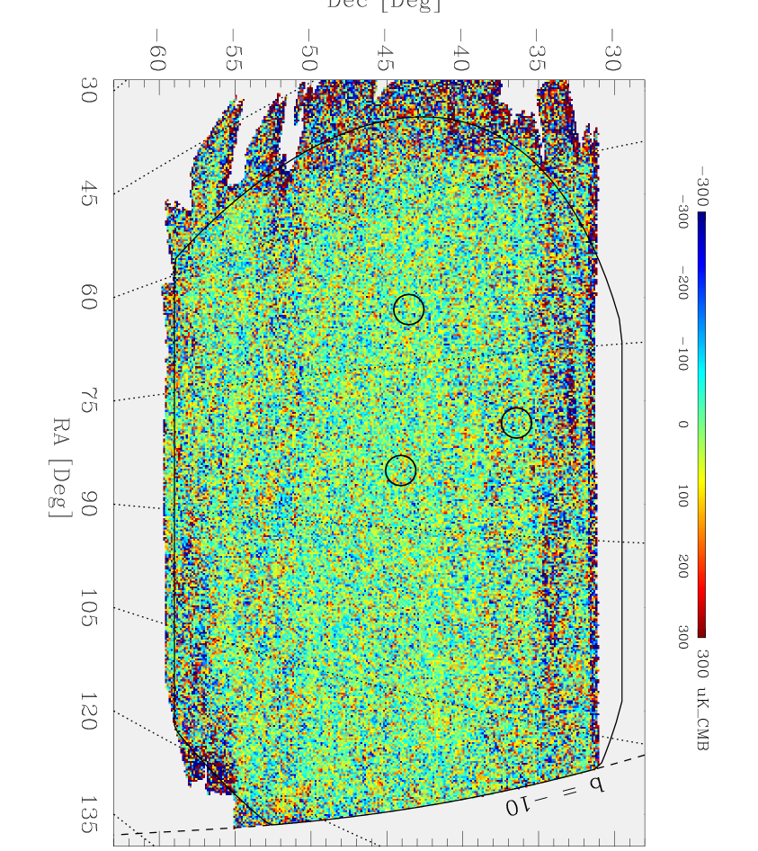
Figure 4: (1dps-2dps) difference maps, both at $7^{\prime}$ pixelization to facilitate map comparisons by eye, for the region of sky where these scans overlap. The color scale is the same as for the previous figures. Note that the consistency test power spectra are calculated on these maps divided by two, (1dps-2dps)/2. Top panel: The MADCAP difference map. This map is not destriped, since in that pipeline the constant-declination stripes are ignored (by introducing a constraint matrix) in the derivation of the angular power spectrum. Bottom panel: The destriped FASTER difference map. Note that the MADCAP input timestream contains additional low frequency information that is removed by an additional highpass filter in the FASTER pipeline.

Figure 5 shows the power spectra of the signal maps (top panel) shown in Figure 2 and of the (1dps-2dps) difference maps (bottom panel) shown in Figure 4. It is apparent that the power spectra of the signal maps are in very good agreement with one another; these are discussed in more detail below. Here we focus on the (1dps-2dps)/2 difference spectra.

The statistical error in the power spectra of the signal maps is dominated by sample variance for $\ell<500$. Because there is no signal and thus no sample variance in the power spectra of the difference maps, the difference maps are sensitive to systematic effects that are well below the (sample variance dominated) statistical noise of the signal maps at low $\ell$.

The FASTER Monte-Carlo simulations show that the different scanning and $\ell$-space filtering in the 1dps and 2dps data leads to a leakage of CMB signal into the (1dps-2dps)/2 FASTER map. The average level of this signal is expected to be at the level of $\sim 10\mu\mbox{K}^{2}$ near the first peak at $\ell\sim 200$. We correct for this effect in the FASTER pipeline consistency test by subtracting the Monte-Carlo mean residual power found in each bin from the actual (1dps-2dps)/2 power spectrum, and by adding the variance of this effect in quadrature to the errors on that power spectrum.

After these corrections to the FASTER pipeline, we find the difference map angular power spectra shown in the bottom panel of Figure 5. The $\chi^{2}$ per degree of freedom with respect to a zero-signal model is 1.34 (1.28) with a probability of exceeding this $\chi^{2}$ of $P_{>}=0.14$ (0.18) for the MADCAP (FASTER) analysis, respectively. Thus, when the entire spectrum is considered, the difference spectra of both analysis methods are reasonably consistent with zero. It is clearly apparent, however, that there is a statistically significant signal in the FASTER difference spectrum, at $\ell\leq 300$. Over this limited range of the spectrum, the FASTER spectrum has a reduced $\chi^{2}=3.7$ for 6 degrees of freedom, for a $P_{>}=0.001$. Over the same range, the MADCAP analysis gives a reduced $\chi^{2}=1.10$ for 6 degrees of freedom, for a $P_{>}=0.36$.

The residual signal in the FASTER difference map is both localized in $\ell$ and very small, with a mean of only $45\mu\mbox{K}^{2}$ in the four bins $150<\ell<300$. The CMB signal is roughly 5000 $\mu\mbox{K}^{2}$ in this $\ell$ range, and our statistical errors on the CMB signal, dominated by sample variance, are $\sim 400\mu\mbox{K}^{2}$. Thus, though the FASTER pipeline formally fails this test, our statistical errors dominate our systematic errors by an order of magnitude.

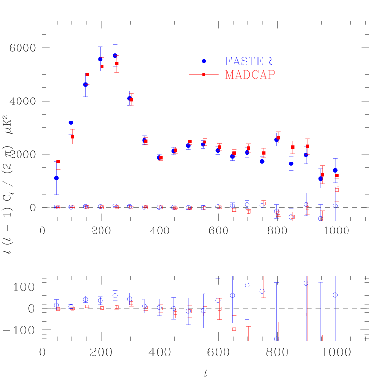
Figure 5: MADCAP and FASTER angular power spectra and (1dps-2dps)/2 difference map power spectra. Top Panel: the FASTER (filled blue circles) and MADCAP (filled red squares) angular power spectra, and their respective (1dps-2dps)/2 difference map power spectra (open symbols). The effects of constant-declination stripes have been removed in each of these analyses. Bottom panel: the difference map angular power spectra plotted on a magnified scale. There is a systematic effect near $\ell\sim 200$ in the FASTER power spectrum, which is absent in the MADCAP treatment. The level of these residuals is much smaller than the statistical errors on the full power spectrum, shown in the top panel.

Investigation of individual detector channels shows that the (1dps-2dps)/2 power spectra near $\ell\sim 200$ are of similar shape and amplitude in each. We have done a variety of other consistency tests and simulations using the FASTER pipeline on our lowest-noise channel, B150A, to try and understand potential sources for the (1dps-2dps)/2 failure. We have broken the data into four quarters (Q1 and Q2 at 1dps; Q3 and Q4 at 2dps) and found difference map power spectra for combinations that minimize effects that depend on scan speed [(Q1+Q3)-(Q2+Q4)] or a drift in time [(Q1+Q4)-(Q2+Q3)]. These combinations fail the consistency test with amplitudes and shapes similar to the (1dps-2dps)/2 failure.

Simulations were done in an attempt to recreate the (1dps-2dps)/2 difference failure by inducing various systematic effects. Changes in the gain, the pointing offset, and the filtering were modeled. Of these, only the last can explain the failure in the FASTER pipeline, given that the data pass the test in the MADCAP pipeline, since gain and pointing offsets should be treated identically by the two methods. For plausible levels of these systematic errors, none induced (1dps-2dps)/2 failures at the level seen. The systematic that created the most similar shape was a pointing offset between the two data sets. This is not a priori unlikely, as it is plausible that a differential offset might occur in the attitude reconstruction for the two scan speeds. The magnitude of the difference test failure would correspond to an $\sim 7^{\prime}$ offset between the two data sets. This is inconsistent with the measured stability of the positions of the quasars in the two maps and, more importantly, is inconsistent with the fact that the MADCAP analysis achieves equally high or higher sensitivity and passes this test. We have not been able to find the cause of the FASTER analysis failure of the (1dps-2dps)/2 consistency test.

We also used the FASTER pipeline to perform two other consistency tests on the real data. These are shown, along with the (1dps-2dps)/2 results for reference, in Figure 6. One differences maps made using rightgoing vs. leftgoing scans. Another compares maps made with two of the four channels (channels A and A2) with the other two (channels A1 and B2). Both of these power spectra appear to be consistent with zero in all $\ell$ regions, as evidenced by the statistics quoted in Table 1.

Figure 6: Difference map power spectra derived using FASTER. The top panel shows the (1dps-2dps)/2 difference map results. The middle panel shows the result found by difference maps made from leftgoing scans and rightgoing scans, (L-R)/2. The bottom panel is for a map made by differencing maps made by two channel combinations, [(A+A2)-(A1+B2)]/2. While the latter two power spectra are relatively consistent with zero contamination, near $\ell\sim 200$ the (1dps-2dps)/2 spectrum is not. This contamination is, however, much smaller than the statistical errors on the full CMB power spectrum in this $\ell$-region. The $\chi^{2}$ statistics of these spectra with respect to zero signal are given in Table 1.

Table 1: Consistency Test Results

Test	bins	Reduced $\chi^{2}$	P>
FASTER (L-R)/2	all	1.15	0.29
	1-6	0.96	0.45
FASTER [(A+A2)-(A1+B2)]/2	all	1.18	0.26
	1-6	1.25	0.28
FASTER (1dps-2dps)/2	all	1.28	0.18
	1-6	3.70	0.001
MADCAP (1dps-2dps)/2	all	1.34	0.14
	1-6	1.11	0.35

Note. — $\chi^{2}$ statistics for the consistency tests described in the text and plotted in Figures 6 and 5. Results are reported for all $\ell$ bins ($50\leq\ell\leq 1000$, 20 bins) as well as for the first six bins ($50\leq\ell\leq 350$), where the FASTER (1-2dps)/2 test failure of Figure 6 is evident.

The (1dps-2dps)/2 test failure on the FASTER pipeline leads us to the inclusion of an additional systematic error term in the region where that failure is significant, ie for $\ell\leq 400$. In our final results below, we increase the quoted FASTER errors on those bins by the amount of the failure, adding it in quadrature (in $\mu\mbox{K}^{2}$) to the likelihood derived errors. In the Fisher matrix this corresponds to adding the difference map power spectrum residuals in quadrature to the diagonal elements, while leaving the off-diagonal terms unmodified.

7 Comparison of results

The discussion above leads us to believe that the larger pixels and the single-beam approximation used by MADCAP should not have a significant effect on the power spectrum. In addition, we have learned of a small consistency test failure over a small range of $\ell$ in the FASTER power spectrum, and corrected the errors on the spectrum accordingly.

We now turn to the comparison of the CMB power spectra derived with FASTER and MADCAP, shown in the top panel of Figure 5.

Despite the fact that they were derived from the same timestream data, there are several reasons why these two power spectra are not expected to be identical. Both the crosslinked observing strategy and the lower frequency filtering cutoff in the timestream allows MADCAP to recover some modes that are missing from the FASTER map.

At the level of the errors shown, the agreement between these two estimates of the power spectrum is excellent. However, there is some indication of a systematic “tilt” between the two spectra. The level of this tilt is not large; modeling it as a difference in the beam window functions, reducing the FWHM of the beam used by MADCAP by one quarter of our systematic beam uncertainty, visually removes the apparent tilt. For this reason, and as is borne out by the discussion below, this difference will not have much effect on the cosmological parameter estimation results.

However, we have investigated any known differences that could lead to a systematic difference between these two power estimation methods. We have shown (via the FASTER consistency tests discussed above) that the larger pixelization and single-beam assumption of MADCAP should not produce such a tilt. Another potential effect is a bias in the pixel window function, which MADCAP takes to be the average HEALPIX window function on the sphere. The FASTER Monte-Carlos incorporate the effects of the real pixel geometries; any bias induced by using a single, isotropized approximation for the smoothing of the HEALPIX pixelization is corrected by Monte-Carlo estimation of the transfer function $F_{\ell}$. In effect the transfer function ensures the method is robust to any similar approximations used in describing the effective pixelization smoothing. However, the analytic arguments discussed above, based on individual pixel window functions calculated for larger pixels, indicate that any such bias caused by the MADCAP assumption should be very small.

Another potential bias could be introduced by the destriping algorithms. We have used Monte-Carlos to test for such effects in FASTER, and have found that any such bias is much smaller than the effect seen here. The marginalization method used by MADCAP is not expected to bias the power spectrum in any way, but Monte-Carlo tests to verify this are not practical given the greater computational cost of that pipeline.

In principle a tilt could also be induced by a difference in the timestream noise statistics used by one of the methods; however, the same noise power spectrum (or time-time noise correlation function) is used by the two pipelines.

It is possible that the constant declination striping is not fully removed by one of the destriping algorithms, and this leads to the difference in tilt. As can be seen in Figure 3, the FASTER destriping does affect the power spectrum slightly at high $\ell$. If this is the reason for the tilt discrepancy, residual striping that is randomly phased with respect to the CMB sky signal would increase the level of the power spectrum.

Figure 7 compares the B02 result, derived using FASTER on 1.9% of the sky at $7^{\prime}$ pixelization, with several new results. The top panel compares the B02 result with the final FASTER result discussed above, on 2.9% of the sky at $3.5^{\prime}$ resolution. The middle panel shows a new MADCAP analysis of the same region as B02, with the same resolution. Finally, in the bottom panel B02 is compared with the MADCAP analysis of the larger cut analyzed in this paper, at $7^{\prime}$ resolution. As expected, the larger dataset leads to smaller errorbars across the entire range of $\ell$. The MADCAP errors are smaller than the FASTER errors at low $\ell$, due to the preservation of lower frequencies in the timestream. The FASTER results agree very well with one another, except in the region near $\ell\sim 800$ where there are three 1-$\sigma$ and one 2-$\sigma$ deviations. In the lower panels there is some evidence for the same tilt bias between MADCAP and FASTER on the B02 cut (mentioned above), indicating this is not unique to the larger sky cut.

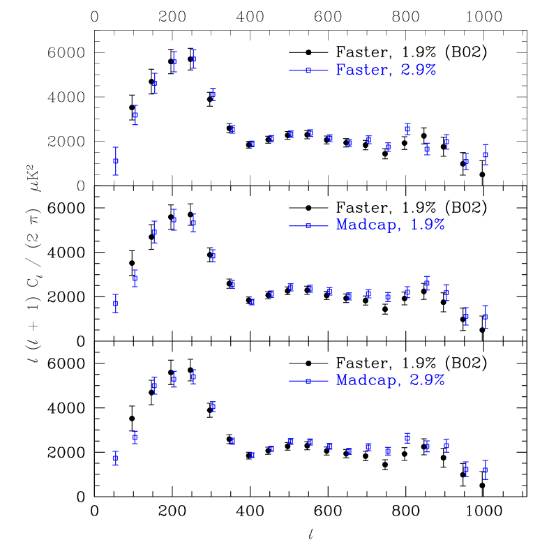
Figure 7: A comparison of the FASTER results of B02 (black filled circles) derived from 1.9% of the sky at $7^{\prime}$ pixelization, with three new analyses (open blue squares in each panel). Top panel: the FASTER results of this paper (2.9% of the sky, $3.5^{\prime}$ pixelization). Middle panel: a new MADCAP analysis of the B02 sky cut (1.9% of the sky, $7^{\prime}$ pixelization). Bottom panel: the MADCAP results of this paper (2.9% of the sky, $7^{\prime}$ pixelization). The agreement is generally very good, with the greatest variations at high $\ell$ where noise, rather than cosmic variance, dominates the errors.

8 Galactic Dust

In Masi et al. (2001) we measured the angular power spectrum of the Boomerang 410 GHz map in three circles of $9^{\circ}$ radius, centered at galactic latitudes of $b=-38^{\circ}$, $-27^{\circ}$ and $-17^{\circ}$. Correlating the lower-frequency Boomerang maps, which are dominated by CMB fluctuations, with the 3000 GHz map of Finkbeiner et al. (1999, model 8 of that paper), gave a measure of the spectral ratios between that map and the Boomerang bands; these ratios were used to scale the 410 GHz power spectra to the lower frequencies.

In the region farthest from the galactic plane, the 410 GHz map is consistent with noise and no dust power spectrum result is reported. Figure 8 shows the extracted power spectrum of dust for the $b=-27^{\circ}$ circle, taken directly from Masi et al. (2001), along with the same calculation for the $b=-17^{\circ}$ circle of that paper. These results show that the dust contribution to the total power spectrum is largest at low $\ell$, and is generally small ($<100\mu$K²).

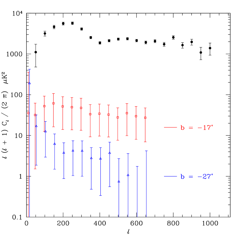
Figure 8: Angular power spectra of IRAS-correlated dust scaled to 150 GHz for two circles of radius $9^{\circ}$ centered at galactic latitudes of $b=-17^{\circ}$ (red open squares) and $b=-27^{\circ}$ (blue open triangles). Details of this analysis can be found in Masi et al. (2001). The FASTER CMB power spectrum (filled black circles) is shown for reference.

A proper estimate of the contribution of dust emission to the measured power spectrum requires the specific morphology of the dust emission be taken into account. We have done this by using the MADCAP analysis path to marginalize over templates of the galactic foregrounds. The results are shown in Figure 9. Here, we have used two templates, one of galactic synchrotron emission (Haslam et al., 1981; Jonas et al., 1998; Finkbeiner, 2002), the other of galactic dust emission (Schlegel et al., 1998; Finkbeiner, 2002). The power spectrum is very stable to this process, with no significant change for $\ell\geq 100$. There is a one sigma change in the power at $\ell=50$, consistent with the the expectation that the effects of dust contamination should be largest at lowest $\ell$, and generally small. We use the galaxy template marginalized MADCAP results in the remainder of this paper. For the FASTER results, for which the statistical errors at low $\ell$ are substantially higher than those of the MADCAP spectrum, the effects of dust emission are negligible.

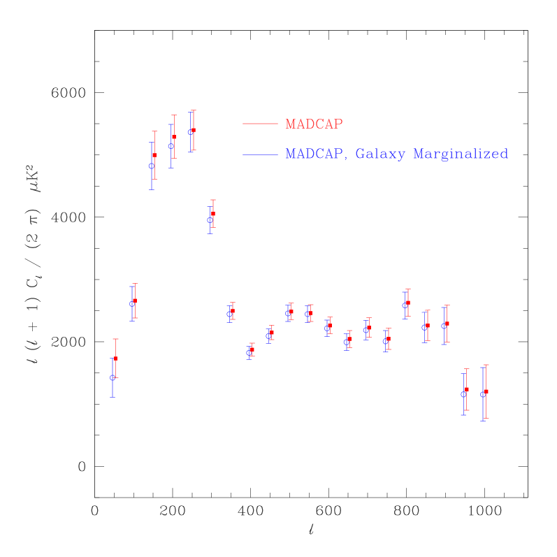
Figure 9: Galactic marginalization. The filled red squares show the results of the MADCAP analysis with marginalization over the constant-declination modes (to remove constant-declination striping). The open blue circles show the results after additional marginalization over two galactic templates, one of galactic dust and the other of galactic synchrotron emission. These lead to slight shifts in the power spectrum at low $\ell$, only significant in the first bin.

9 Final Results

We have used FASTER and MADCAP to derive two estimates of the angular power spectrum using the same input timestream, sky coverage, and noise statistics. The final FASTER results, derived from a $3.5^{\prime}$ pixel map and corrected for the small (1dps-2dps)/2 consistency test failure, appear along with the final galaxy-marginalized MADCAP results in Figure 10.

Our power spectrum results are characterized by a likelihood function for the bandpower in each band (${\cal C}_{b}$). A good approximation to this function is given by an offset lognormal function (Bond et al., 1998) $Z_{b}=\ln(\overline{{\cal C}}_{b}+x_{b})$ of the maximum likelihood values found in each band ($\overline{{\cal C}}_{b}$) and an offset parameter for each band, $x_{b}$. Given these, the likelihood is found by

$$\sigma_{b} = \Delta\overline{{\cal C}}_{b}/(\overline{{\cal C}}_{b}+x_{b})$$ (6)

$$\Delta Z_{b} = \ln({\cal C}_{b}+x_{b})-\ln(\overline{{\cal C}}_{b}+x_{b})$$ (7)

$$-2\ln L({\cal C}_{b}) = \sum_{bb^{\prime}}\Delta Z_{b}\sigma_{b}^{-1}G_{bb^{\prime}}\sigma_{b^{\prime}}^{-1}\Delta Z_{b^{\prime}}$$ (8)

where $G_{bb^{\prime}}$ is the bandpower correlation matrix, normalized to unity on the diagonal. Table 2 gives the maximum likelihood value $\overline{{\cal C}}_{b}=\ell(\ell+1)C_{\ell}/2\pi$, curvature error ($\Delta\overline{{\cal C}}_{b}$), and offset parameter $x_{b}$ for each band for both the FASTER and MADCAP results of Figure 10. The bin-bin correlation matrices for these power spectra are given in Tables 3 and 4 for FASTER and MADCAP respectively. These data, and the window functions of Figure 12, are available at http://cmb.phys.cwru.edu/boomerang/ or http://oberon.roma1.infn.it/boomerang.

One measure of the level of agreement between the FASTER and MADCAP power spectra can be made by treating the two power spectra as independent datasets (which they are not) and using the curvature errorbars to calculate a chi-square statistic. We find that $\chi^{2}=8.54$ for 20 degrees of freedom, which gives $P_{>}=0.988$. This low $\chi^{2}$ value indicates that the two analyses of the same data vary by an amount much less than is expected for two random realizations of the same measurement. That is, the “analysis variance” is very small compared to the statistical errors.

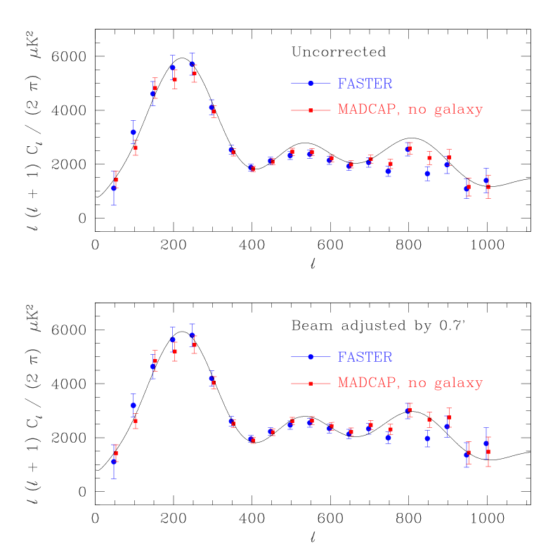
Figure 10: Final angular power spectrum results at 150 GHz, also given in Table 2. In both panels, the MADCAP results are shown as red squares, while the FASTER results are given as blue circles. The top panel shows the data of Table 2, along with the best-fit model from the weak-prior parameter estimation discussed below. In addition to the errors shown, there is a 10% uncertainty in the temperature calibration (20% in the temperature-squared units of this plot), and a beam uncertainty of $1.4^{\prime}$ rms. In the bottom panel we have rescaled the data by changing the the beam window function by 0.5$\sigma$. This gives much better visual agreement with the model.

Table 2: Angular Power Spectra.

		FASTER				MADCAP
$\ell_{low}$	$\ell_{high}$	$\overline{{\cal C}}_{b}$	$\Delta\overline{{\cal C}}_{b}$	$x_{b}$		$\overline{{\cal C}}_{b}$	$\Delta\overline{{\cal C}}_{b}$	$x_{b}$
26	75	1053	401	22		1423	313	341
76	125	3175	358	40		2609	279	34
126	175	4614	406	71		4823	384	50
176	225	5581	418	110		5139	349	81
226	275	5710	385	162		5365	321	124
276	325	4107	264	228		3953	222	180
326	375	2532	160	320		2445	137	249
376	425	1877	120	441		1822	105	337
426	475	2120	130	593		2092	116	467
476	525	2320	142	794		2456	132	638
526	575	2368	149	1054		2444	135	854
576	625	2141	147	1397		2216	133	1133
626	675	1923	149	1838		1994	136	1497
676	725	2066	170	2437		2186	157	2023
726	775	1738	184	3202		2008	172	2657
776	825	2551	239	4204		2581	217	3669
826	875	1647	252	5542		2229	245	4837
876	925	1976	312	7237		2253	296	6674
926	975	1087	352	9696		1156	334	8560
976	1025	1394	444	12878		1155	430	12324

Note. — Angular power spectra of the CMB, derived using the FASTER (columns 3-5) and MADCAP (columns 6-8) methods. The FASTER power spectrum has been corrected for the (1-2dps)/2 failure by the addition of a systematic errorbar in quadrature with the statistical one in the relevant $\ell$ bins. The MADCAP power spectrum has been marginalized over two galactic templates as discussed in the text. The FASTER power spectrum is calculated for shaped bins, while the MADCAP power spectrum is calculated for tophat bins.

Table 3: FASTER Bandpower Correlation Matrix

1	2	3	4	5	6	7	8	9	10	11	12	13	14	15	16	17	18	19	20
1.000	-0.140	0.005	-0.002	0	0	0	0	0	0	0	0	0	0	0	0	0	0	0	0
-	1.000	-0.089	0	-0.004	-0.004	-0.005	-0.007	-0.006	-0.005	-0.006	-0.006	-0.007	-0.007	-0.007	-0.006	-0.006	-0.005	-0.005	-0.004
-	-	1.000	-0.088	-0.001	-0.006	-0.006	-0.007	-0.007	-0.006	-0.005	-0.006	-0.006	-0.006	-0.007	-0.005	-0.006	-0.005	-0.005	-0.004
-	-	-	1.000	-0.087	-0.003	-0.008	-0.008	-0.006	-0.006	-0.005	-0.005	-0.006	-0.005	-0.005	-0.005	-0.005	-0.004	-0.004	-0.004
-	-	-	-	1.000	-0.088	-0.005	-0.009	-0.006	-0.004	-0.004	-0.004	-0.004	-0.004	-0.004	-0.003	-0.004	-0.003	-0.003	-0.003
-	-	-	-	-	1.000	-0.090	-0.004	-0.005	-0.003	-0.003	-0.003	-0.002	-0.002	-0.002	-0.002	-0.002	-0.002	-0.002	-0.002
-	-	-	-	-	-	1.000	-0.088	0	-0.003	-0.002	-0.001	-0.001	-0.001	-0.001	0	0	0	0	0
-	-	-	-	-	-	-	1.000	-0.085	0	-0.003	-0.002	-0.001	0	0	0	0	0	0	0
-	-	-	-	-	-	-	-	1.000	-0.088	0	-0.003	-0.002	-0.001	-0.001	0	0	0	0	0
-	-	-	-	-	-	-	-	-	1.000	-0.089	0	-0.003	-0.002	-0.001	0	0	0	0	0
-	-	-	-	-	-	-	-	-	-	1.000	-0.089	0	-0.003	-0.002	0	0	0	0	0
-	-	-	-	-	-	-	-	-	-	-	1.000	-0.087	0	-0.003	-0.001	0	0	0	0
-	-	-	-	-	-	-	-	-	-	-	-	1.000	-0.084	0	-0.003	-0.001	0	0	0
-	-	-	-	-	-	-	-	-	-	-	-	-	1.000	-0.086	0	-0.003	-0.001	0	0
-	-	-	-	-	-	-	-	-	-	-	-	-	-	1.000	-0.088	0.001	-0.003	-0.001	0
-	-	-	-	-	-	-	-	-	-	-	-	-	-	-	1.000	-0.091	0	-0.003	-0.001
-	-	-	-	-	-	-	-	-	-	-	-	-	-	-	-	1.000	-0.088	0	-0.003
-	-	-	-	-	-	-	-	-	-	-	-	-	-	-	-	-	1.000	-0.087	0
-	-	-	-	-	-	-	-	-	-	-	-	-	-	-	-	-	-	1.000	-0.081
-	-	-	-	-	-	-	-	-	-	-	-	-	-	-	-	-	-	-	1.000

Note. — The FASTER CMB power spectrum band-band correlation matrix, $G_{bb^{\prime}}$ of equation 8. This matrix is symmetric; values below the diagonal, not printed, are symmetric with those above. Values with magnitude $0.0005$ and lower have been truncated to zero. Bands are labelled 1-20 in consecutive order from low to high $\ell$, as given in Table 2.

Table 4: MADCAP Bandpower Correlation Matrix

1	2	3	4	5	6	7	8	9	10	11	12	13	14	15	16	17	18	19	20
1.000	-0.080	-0.001	-0.002	0	0	0	0	0	0	0	0	0	0	0	0	0	0	0	0
-	1.000	-0.058	-0.001	-0.001	0	0	0	0	0	0	0	0	0	0	0	0	0	0	0
-	-	1.000	-0.057	-0.001	-0.001	0	0	0	0	0	0	0	0	0	0	0	0	0	0
-	-	-	1.000	-0.056	0	-0.001	0	0	0	0	0	0	0	0	0	0	0	0	0
-	-	-	-	1.000	-0.055	0	-0.001	0	0	0	0	0	0	0	0	0	0	0	0
-	-	-	-	-	1.000	-0.055	0	-0.001	0	0	0	0	0	0	0	0	0	0	0
-	-	-	-	-	-	1.000	-0.056	0	-0.001	0	0	0	0	0	0	0	0	0	0
-	-	-	-	-	-	-	1.000	-0.055	0	-0.002	0	0	0	0	0	0	0	0	0
-	-	-	-	-	-	-	-	1.000	-0.054	0	-0.002	0	0	0	0	0	0	0	0
-	-	-	-	-	-	-	-	-	1.000	-0.054	0	-0.002	0	0	0	0	0	0	0
-	-	-	-	-	-	-	-	-	-	1.000	-0.054	-0.001	-0.002	0	0	0	0	0	0
-	-	-	-	-	-	-	-	-	-	-	1.000	-0.055	-0.001	-0.002	0	0	0	0	0
-	-	-	-	-	-	-	-	-	-	-	-	1.000	-0.055	-0.002	-0.002	-0.001	0	0	0
-	-	-	-	-	-	-	-	-	-	-	-	-	1.000	-0.056	-0.002	-0.002	-0.001	0	0
-	-	-	-	-	-	-	-	-	-	-	-	-	-	1.000	-0.056	-0.002	-0.002	-0.001	0
-	-	-	-	-	-	-	-	-	-	-	-	-	-	-	1.000	-0.057	-0.002	-0.002	-0.001
-	-	-	-	-	-	-	-	-	-	-	-	-	-	-	-	1.000	-0.058	-0.002	-0.002
-	-	-	-	-	-	-	-	-	-	-	-	-	-	-	-	-	1.000	-0.060	-0.003
-	-	-	-	-	-	-	-	-	-	-	-	-	-	-	-	-	-	1.000	-0.061
-	-	-	-	-	-	-	-	-	-	-	-	-	-	-	-	-	-	-	1.000

Note. — The MADCAP CMB power spectrum band-band correlation matrix, $G_{bb^{\prime}}$ of equation 8. This matrix is symmetric; values below the diagonal, not printed, are symmetric with those above. Values with magnitude $0.0005$ and lower have been truncated to zero. Bands are labelled 1-20 in consecutive order from low to high $\ell$, as given in Table 2.

10 Features in the Power Spectrum

The cosmological parameter estimation procedure we follow below is done in the context of inflation-motivated models with adiabatic initial density perturbations. Thus, it is both interesting and important to assess the evidence in favor of these models. One of their generic predictions is that there will be a series of peaks in the CMB power spectrum, the exact positions and amplitudes of which depend on the cosmological parameters. It is thus interesting to search for such features in our power spectrum and evaluate the statistical significance with which they are detected.

To detect such features, we use the method applied to the B02 power spectrum in de Bernardis et al. (2002), based on parabolic fits to the CMB power spectrum over a fixed number of bands. We fit the spectrum to the polynomial

$${\cal C}_{\ell}={\cal C}_{A}(\ell-\ell_{p})^{2}+{\cal C}_{B},$$ (9)

where $\ell_{p}$ is the peak position. In order to fit the measured bandpowers $\overline{\cal C}_{b}$ we average the model ${\cal C}_{\ell}$ over the bands reported in Table 2, thus obtaining the theoretical bandpowers ${\cal C}_{b}^{T}$. Using the covariance matrix $G^{-1}_{bb^{{}^{\prime}}}$ of the measured bandpowers we compute

$$\chi^{2}=(\overline{{\cal C}}_{b}-{\cal C}_{b}^{T})G^{-1}_{bb^{\prime}}(\overline{{\cal C}}_{b^{\prime}}-{\cal C}_{b^{\prime}}^{T}),$$ (10)

which we minimize by varying ${\cal C}_{A}$, ${\cal C}_{B}$ and $\ell_{p}$. Errors on the fit $\ell_{p}$ and ${\cal C}_{B}$ are found by marginalization of the full likelihood over ${\cal C}_{A}$. In order to evaluate the significance of the detection of a feature we study the likelihood of the curvature ${\cal C}_{A}$ marginalizing over the other two parameters.

When we compare different models, i.e. different values of the two parameters $\ell_{p}$ and ${\cal C}_{B}$, the $\chi^{2}$ has 2 degrees of freedom. In order to show how other models compare to the best-fit one, we plot in Figure 11 the contours corresponding to $\Delta\chi^{2}=2.3,6.17,11.8$, i.e. $68.3\%,95.4\%$ and $99.7\%$ confidence.

Table 5 shows the results of this analysis for both the MADCAP and the FASTER power spectra of Table 2. The significance of the detections depends somewhat on the range of bands over which the fit is done; the results in the table are those that give the most significant detections. Comparing the results to de Bernardis et al. (2002) we find a general improvement in the precision with which the peaks and valleys are located, particularly for the first and second peaks, and for the first valley. We obtain very similar results in a variation of this method where a three-parameter quadratic is fit over a sliding five-band window, also described in de Bernardis et al. (2002). The results are also very similar when applied to a FASTER power spectrum derived for bands of the same width ($\Delta\ell=50$) with band centers shifted by $\ell=25$.

In order to investigate the level at which the detections of different peaks are correlated, we have performed a simultaneous fit of all the spectral bins using a linear combination of four Gaussians

$${\cal C}_{\ell}=\sum_{i=1}^{4}A_{i}^{2}\exp(-(\ell-\ell_{i})^{2}/2\sigma_{i}^{2}),$$ (11)

which is sufficiently flexible to provide a good fit to any standard theoretical spectrum. We proceed using a Monte-Carlo Markov Chain method, as in Christensen et al. (2001), Lewis & Bridle (2002), and Odman et al. (2002), accounting for calibration and beam uncertainties as in Bridle et al. (2002). We find best fit values for $A_{i}$ and $\ell_{i}$ that are in good agreement with the results obtained above, and point clearly towards the presence of features in the power spectrum.

Using this simultaneous fit to all of the power spectrum bins with a single phenomenological function allows us to study the correlation between the different parameters. These are not negligible between the amplitudes of the peaks that are near to each other (for example $R(A_{1},A_{2})=0.19$; $R(A_{1},A_{3})=0.07$, $R(A_{2},A_{3})=0.27$), and between amplitudes and widths ($R(A_{1},\sigma_{1})=0.20$), but the detections are all confirmed.

As the table and figure show, we clearly detect multiple features in the power spectrum. The next question is whether the adiabatic perturbation, inflationary model set can produce models with similar features.

Using the same methods discussed below for cosmological parameter estimation, we use the data and our theoretically motivated database of ${\cal C}_{\ell}$ models to make Bayesian estimates of the positions and amplitudes of peaks in the power spectrum, for comparison with our model-independent fits. The last two columns of Table 5 show the results of this process (using the “weak prior” described below), and give results that agree very well with the phenomenologically measured parameters of the various features. This bolsters our confidence in the model set we use in the next section, to estimate cosmological parameters.

Table 5: Peaks and Valleys in the CMB

			MADCAP				FASTER				Adiabatic CDM
Feature	$\ell$ range		$\ell_{\rm p}$	${\cal C}_{\rm p}$ ($\mu K^{2}$)	level		$\ell_{\rm p}$	${\cal C}_{\rm p}$ ($\mu K^{2}$)	level		$\ell_{\rm p}$	${\cal C}_{\rm p}$ ($\mu K^{2}$)
Peak 1	$100-300$		$216^{+6}_{-5}$	$5480^{+1130}_{-1130}$	$6.7\sigma$		$215^{+5}_{-6}$	$5690^{+1200}_{-1200}$	$4.8\sigma$		$223^{+4}_{-4}$	$6022^{+394}_{-370}$
Valley 1	$300-500$		$425^{+4}_{-5}$	$1820^{+420}_{-410}$	$6.3\sigma$		$430^{+7}_{-5}$	$1870^{+420}_{-410}$	$4.3\sigma$		$411^{+17}_{-17}$	$1881^{+152}_{-141}$
Peak 2	$400-650$		$536^{+10}_{-10}$	$2420^{+620}_{-570}$	$4.0\sigma$		$528^{+14}_{-10}$	$2330^{+600}_{-550}$	$3.1\sigma$		$539^{+19}_{-19}$	$2902^{+248}_{-229}$
Valley 2	$550-800$		$673^{+18}_{-13}$	$2030^{+670}_{-560}$	$2.6\sigma$		$681^{+21}_{-21}$	$1910^{+630}_{-530}$	$2.5\sigma$		$667^{+28}_{-27}$	$2122^{+302}_{-265}$
Peak 3	$750-950$		$825^{+10}_{-13}$	$2500^{+1100}_{-840}$	$3.2\sigma$		$820^{+15}_{-22}$	$2150^{+1000}_{-720}$	$2.2\sigma$		$812^{+26}_{-25}$	$3121^{+497}_{-429}$

Note. — Locations and amplitudes of peaks and valleys in the power spectrum of the CMB, obtained with polynomial fits. The locations, amplitudes, and confidence levels of detection are listed for MADCAP (columns 3-5) and FASTER (columns 6-8). The $\ell$ range used in the parabolic analysis is reported in column 2. Columns 9 and 10 gives the result of cosmological “peak parameter” extraction (using the MADCAP data, COBE-DMR data, and the “weak cosmological prior” discussed below) from the set of adiabatic perturbation, cold dark matter models used in our cosmological parameter estimation. All the errors include the effects of gain and beam calibration uncertainties.

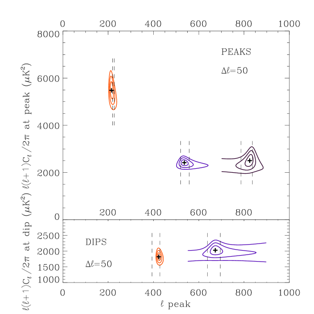
Figure 11: $\Delta\chi^{2}$ contours for the position and amplitude of peaks and valleys in the Boomerang MADCAP power spectrum. The contours are at $\Delta\chi^{2}=2.3,6.17,11.8$, i.e. 68.3%, 95.4% and 99.7% confidence. The vertical dashed lines give the feature positions found using the cosmological database, and as given in Table 5. Similar results are obtained using the FASTER results.

11 Cosmological Parameters

Our measurement of the CMB angular power spectrum can be used in conjunction with other cosmological information to constrain several cosmological parameters. Our method, described in detail in Lange et al. (2001), compares the measured angular power spectrum with the predicted power spectra from a family of theoretical models. We choose to compare our measurements with inflation-motivated adiabatic cold dark matter models, with the 7 cosmological parameters given in Table 6.

We take a Bayesian approach, calculating a likelihood of each model given the data, in the discrete parameter database of Table 6. We then marginalize over the continuous parameters such as theory normalization ($\ln{\cal C}_{10}$), calibration, and beam uncertainty for each model. To find confidence intervals on any given parameter, we marginalize over the other parameters by integrating through the database, collapsing the n-dimensional likelihood to a one-dimensional likelihood curve for that parameter.

In the comparison of the theoretical and measured power spectra, one must convolve the predicted theory power spectrum with the window function for each $\ell$ bin of the measurement. The flat band average of a target model ${\cal C}^{T}_{\ell}=\ell(\ell+1)C^{T}_{\ell}/2\pi$, can be defined with respect to a window function $W^{b}_{\ell}$ for that band as

$${\cal C}^{T}_{b}=\frac{{\cal I}[W^{b}_{\ell}{\cal C}^{T}_{\ell}]}{{\cal I}[W^{b}_{\ell}]}$$ (12)

with

$${\cal I}[f_{\ell}]=\sum_{\ell}\frac{(\ell+\frac{1}{2})}{\ell(\ell+1)}f_{\ell}.$$ (13)

In the power spectrum estimation pipelines discussed above, we can choose to use shaped bands rather than flat. This will change the details of the window function, but the prescription for calculating theoretical band averages remains the same.

We have calculated the window functions for the FASTER power spectrum bins, using S+N weighting on the map. In Figure 12 we show the flat-band window functions, to illustrate their $\ell$-space shapes and the level of correlations between bands. Details on their derivation are given in Contaldi et al. (2002). For the MADCAP comparison with theory, we use tophat window functions.

Figure 12: Window functions derived from the FASTER analysis. These window functions are used to relate a continuous theoretical model to the expected experimental band powers, a crucial step in parameter extraction. The functions are orthogonal, as a result of the top-hat binning assumed in the theory. The window for the first band shows how all the information is coming from the $50<\ell<76$ region due to the sharp filtering applied (in the FASTER pipeline) to the timestream.

Table 6: Cosmological Parameters Database

Parameter	Values
$\Omega_{k}$	-0.5, -0.3, -0.2, -0.15, -0.1, -0.05, 0, 0.05, 0.1, 0.15, 0.2, 0.3, 0.5, 0.7, 0.9
$\Omega_{\Lambda}$	0, 0.1, 0.2, 0.3, 0.4, 0.5, 0.6, 0.7, 0.8, 0.9, 1.0, 1.1
$\omega_{c}$	0.03, 0.06, 0.08, 0.10, 0.12, 0.14, 0.17, 0.22, 0.27, 0.33, 0.40, 0.55, 0.8
$\omega_{b}$	0.003125, 0.00625, 0.0125, 0.0175, 0.020, 0.0225, 0.025, 0.030, 0.035,
	0.04, 0.05, 0.075, 0.10, 0.15, 0.2
$n_{s}$	0.5, 0.55, 0.6, 0.65, 0.7, 0.725, 0.75, 0.775, 0.8, 0.825, 0.85, 0.875, 0.9,
	0.925, 0.95, 0.975, 1.0, 1.025, 1.05, 1.075, 1.1, 1.125, 1.15, 1.175, 1.2,
	1.25, 1.3, 1.35, 1.4, 1.45, 1.5
$\tau_{c}$	0, 0.025, 0.05, 0.075, 0.1, 0.15, 0.2, 0.3, 0.4, 0.5, 0.7
$\ln{{\cal}C_{10}}$	Continuous

Note. — The values of the cosmological parameters in our model space; while $\ln{C_{10}}$ is marginalized as a continuous variable, the rest are calculated on a grid with the discrete parameter values given. The curvature $\Omega_{k}$ is related to the overall density by $\Omega_{k}=1-\Omega_{total}$. The cold dark matter and baryon physical densities $\omega_{c}$ and $\omega_{b}$ are given by $\omega_{x}=\Omega_{x}h^{2}$, where $h$ is the Hubble parameter in units of 100 km/s/MPc. The database is restricted to models for which $\Omega_{M}$ = $\Omega_{c}+\Omega_{b}>$ 0.1. $n_{s}$ is the spectral index for primordial density fluctuations, where a value of 1.0 indicates scale invariance. Reionization is parameterized by $\tau_{c}$, the Thompson depth to the epoch when the universe reionized after photon decoupling. In addition to these cosmological parameters, there are instrumental parameters describing the systematic gain and beam uncertainties. These are accounted for, by marginalization, in all cosmological parameter estimates reported in this paper.

We can also apply a series of “priors”, or prior probabilities, to each model in the database, modifying the likelihood of that model before marginalization. The priors we choose include a “weak prior” which sets the likelihood to zero if, for that model, the Hubble parameter ($H_{o}=100h$km/s/MPc) has a value outside the range $0.45<h<0.90$, the current age of the universe is less than 10 Gyr, or the total matter content $\Omega_{M}<0.1$. We also investigate the effect of narrowing the prior on the Hubble constant to $h=0.72\pm 0.08$, as measured by the Hubble Key Project (Freedman et al., 2001).

We also examine the effect of a large-scale structure (LSS) prior. This is a joint constraint on $\sigma_{8}^{2}$, the bandpower of (linear) density fluctuations on a scale corresponding to rich clusters of galaxies ($8h^{-1}$MPc), and on a shape parameter $\Gamma_{\rm eff}$ characterizing the (linear) density power spectrum. The LSS prior probability distribution, described in detail in Bond et al. (2002), is slightly modified over that used in Lange et al. (2001) to agree better with weak lensing and clustering data. $\sigma_{8}\Omega_{m}^{0.56}$ = $0.47^{+.02,+.11}_{-.02,-.08}$, is distributed as a Gaussian (first error) convolved with a uniform (top-hat) distribution (second error), centered about 0.47; $\Gamma_{\rm eff}$ = $0.21^{+.03,+.08}_{-.03,-.08}$ is a broad distribution over the 0.1 to 0.3 range. Here $\Gamma_{\rm eff}$ = $\Gamma+(n_{s}-1)/2$, where $\Gamma\approx\Omega_{m}h\,\exp[-\Omega_{B}(1+\Omega_{m}^{-1}(2{h})^{1/2})]$ is a function of our basic cosmological parameters.

Our final set of priors combines the weak and LSS priors with the supernova data of Riess et al. (1998) and Perlmutter et al. (1999), and the assumption that the geometry of space is flat. In all cases, we use the COBE-DMR measurements (Bennett et al., 1996) to provide a valuable low-$\ell$ anchor for the power spectrum.

We are interested in the robustness of our parameter extraction to the details of the input power spectrum. Specifically, we would like to know if the small differences between different variations of the FASTER analysis, or between the final FASTER and MADCAP power spectra, lead to significant differences in cosmological results. In Figure 13 we show likelihood curves for six cosmological parameters derived using only the weak prior case, for several input versions of our angular power spectrum results. In all cases the likelihood curves are very similar, indicating the cosmological results are not very sensitive to the details of our analysis.

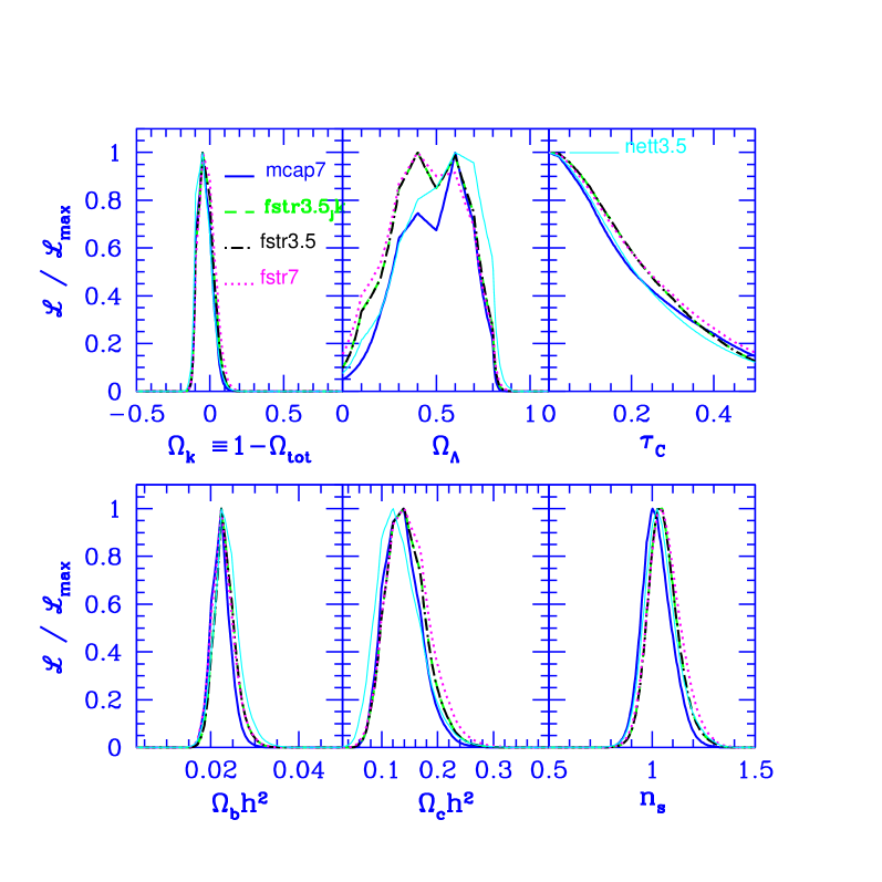
Figure 13: Parameters extracted from our data plus the COBE-DMR results (Bennett et al., 1996), using two “weak” priors, $0.4<h<0.9$ and age $>10$ Gyr. These likelihood curves are quite insensitive to variations in the method or details of the analysis, and show that our analysis methods are quite robust. The green dashed curve shows the FASTER results of Table 2, while the solid blue shows the MADCAP results of that same table. The black dot-dash curve shows the FASTER result with no correction for the (1dps-2dps)/2 consistency test failure. The magenta dotted curve shows the results upon degrading the FASTER analysis to $7^{\prime}$ resolution. The cyan solid curve shows the (FASTER derived) B02 results, using less timestream data and sky coverage as discussed in the text.

Having demonstrated the stability of our results, we now turn to extracting cosmological parameters from our angular power spectrum with the series of applied priors discussed above. Figures 14 and Figures 15 show a set of one dimensional likelihood curves for six parameters, derived from the data of Table 2, COBE-DMR, and the priors described above. Inspection of these figures shows that the parameter likelihoods derived from the FASTER and MADCAP results are very similar for each set of priors. This again demonstrates the stability of the cosmological results to the chosen analysis path. Numerical estimates of parameters derived from these curves are given in Table 6, where a similar comparison can be made.

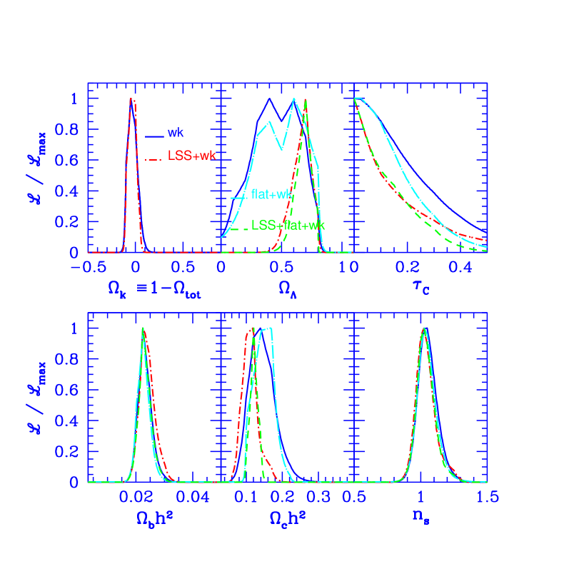
Figure 14: Likelihood curves for six cosmological parameters, derived from the FASTER power spectrum of Table 2 and COBE-DMR, for a series of applied priors described in the text. The solid blue curve is for the “weak prior” case. The dot-dash red line adds the LSS prior to the weak prior. The cyan dot-dash curve is for the “weak prior” case with the added assumption that the geometry is flat. The green dashed curve adds to this the LSS prior. Three parameters, $\Omega_{k}$, $\Omega_{b}h^{2}$, and $n_{s}$ are very well determined and unaffected by the choice of prior. $\Omega_{c}h^{2}$ is fairly well localized by the weak and weak+flat cases, but much better determined when an LSS prior is applied. Similarly, the limits on $\tau_{c}$ improve with the use of the LSS prior. The data favor a non-zero $\Omega_{\Lambda}$ in the weak and weak+flat cases; the use of an LSS prior leads to a very solid detection. In all cases, the observed parameters are consistent with a flat, $\Lambda$-CDM cosmology.

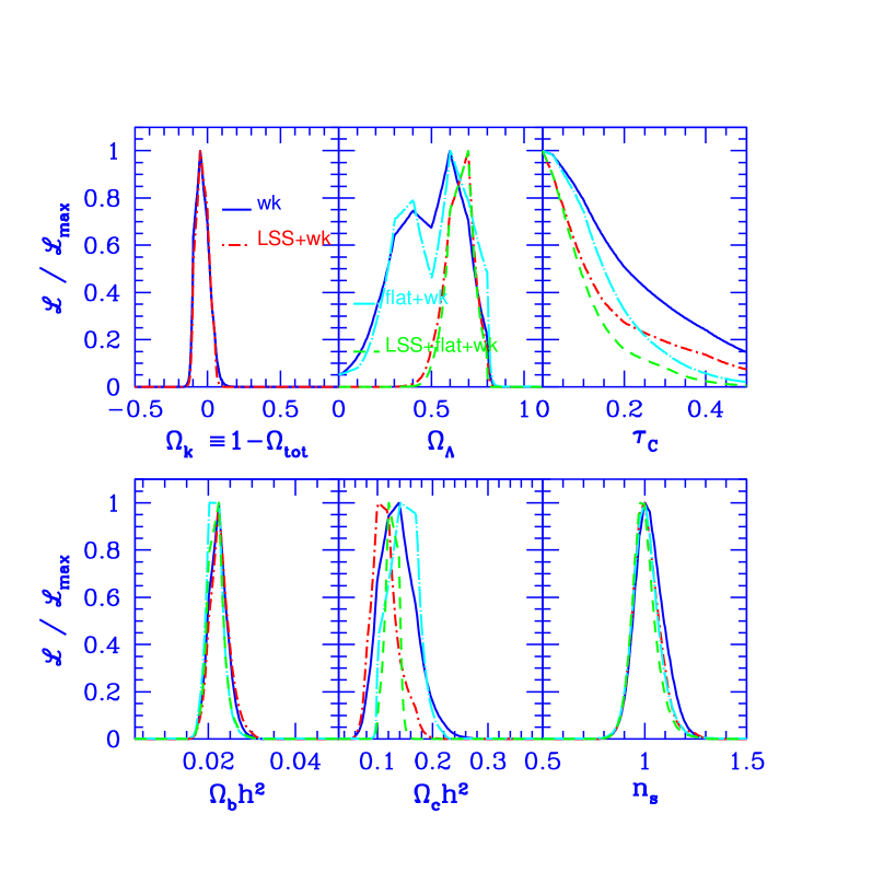
Figure 15: Likelihood curves for six cosmological parameters, derived from the MADCAP power spectrum of Table 2 and COBE-DMR, for a series of applied priors described in the text. The curves are as in Figure 14, and lead to the same conclusions. The agreement of the curves in this figure with those in Figure 14 demonstrates the insensitivity of our analysis to the details of the CMB angular power spectrum estimation pipeline.

Table 7: Parameter Estimates

Priors	Analysis Path	$\Omega_{tot}$	$n_{s}$	$\Omega_{b}h^{2}$	$\Omega_{cdm}h^{2}$	$\Omega_{\Lambda}$	$\Omega_{m}$	$\Omega_{b}$	$h$	Age	$\tau_{c}$
Weak $h$ + age
	MADCAP	$1.04^{0.05}_{0.06}$	$1.02^{0.08}_{0.07}$	$0.023^{0.003}_{0.003}$	$0.14^{0.04}_{0.04}$	$0.50^{0.18}_{0.21}$	$0.55^{0.19}_{0.19}$	$0.077^{0.023}_{0.023}$	$0.56^{0.10}_{0.10}$	$14.8^{1.4}_{1.4}$	$<0.52$
	FASTER	$1.03^{0.05}_{0.06}$	$1.05^{0.08}_{0.07}$	$0.023^{0.003}_{0.003}$	$0.14^{0.04}_{0.04}$	$0.46^{0.21}_{0.21}$	$0.58^{0.21}_{0.21}$	$0.080^{0.025}_{0.025}$	$0.56^{0.11}_{0.11}$	$14.5^{1.5}_{1.5}$	$<0.51$
Weak $h$ + age + LSS
	MADCAP	$1.03^{0.05}_{0.05}$	$1.01^{0.07}_{0.06}$	$0.023^{0.003}_{0.003}$	$0.11^{0.03}_{0.02}$	$0.66^{0.07}_{0.09}$	$0.38^{0.10}_{0.10}$	$0.065^{0.020}_{0.020}$	$0.61^{0.11}_{0.11}$	$14.9^{1.7}_{1.7}$	$<0.50$
	FASTER	$1.03^{0.05}_{0.05}$	$1.03^{0.08}_{0.07}$	$0.024^{0.004}_{0.003}$	$0.11^{0.03}_{0.03}$	$0.68^{0.07}_{0.10}$	$0.36^{0.11}_{0.11}$	$0.066^{0.022}_{0.022}$	$0.63^{0.11}_{0.11}$	$14.8^{1.7}_{1.7}$	$<0.53$
($h=0.72\pm 0.08$) + age
	MADCAP	$1.00^{0.04}_{0.04}$	$1.02^{0.08}_{0.07}$	$0.023^{0.003}_{0.003}$	$0.13^{0.04}_{0.03}$	$0.64^{0.11}_{0.14}$	$0.38^{0.13}_{0.13}$	$0.053^{0.016}_{0.016}$	$0.66^{0.09}_{0.09}$	$13.7^{1.3}_{1.3}$	$<0.49$
	FASTER	$0.99^{0.04}_{0.05}$	$1.06^{0.09}_{0.07}$	$0.023^{0.003}_{0.003}$	$0.14^{0.05}_{0.04}$	$0.62^{0.12}_{0.17}$	$0.39^{0.14}_{0.14}$	$0.055^{0.016}_{0.016}$	$0.67^{0.09}_{0.09}$	$13.4^{1.3}_{1.3}$	$<0.49$
Flat+ Weak $h$ + LSS + SN
	MADCAP	(1.00)	$1.01^{0.06}_{0.05}$	$0.022^{0.002}_{0.002}$	$0.12^{0.02}_{0.01}$	$0.69^{0.04}_{0.06}$	$0.31^{0.05}_{0.05}$	$0.047^{0.005}_{0.005}$	$0.69^{0.04}_{0.04}$	$13.6^{0.4}_{0.4}$	$<0.30$
	FASTER	(1.00)	$1.04^{0.06}_{0.06}$	$0.024^{0.003}_{0.002}$	$0.12^{0.01}_{0.01}$	$0.70^{0.05}_{0.05}$	$0.30^{0.05}_{0.05}$	$0.048^{0.005}_{0.005}$	$0.70^{0.05}_{0.05}$	$13.6^{0.4}_{0.4}$	$<0.31$

Note. — Cosmological parameter estimates for the FASTER and MADCAP results, derived using a series of more restrictive applied priors. The results show remarkable consistency between the two analysis paths, for all priors. The least stable parameter is $n_{s}$, with fairly consistent 1/2 $\sigma$ variations between the two results.

12 Conclusions

In this paper we have presented an analysis of 50% more data from the 1998 Antarctic flight of Boomerang than previously treated. Our analysis is the most thorough to date, using two very different power spectrum estimation pipelines to derive the angular power spectrum of the cosmic microwave background radiation. The two methods show good agreement and, with the greater amount of data used, an increase in the precision of measured power spectrum. In particular, features in the power spectrum beyond the first peak (at $\ell\sim 200$) are detected with greater confidence. Given that such features are a natural consequence of standard cold dark matter dominated cosmological models with adiabatic initial density perturbations, their presence gives us greater confidence in the validity of that model set.

Within the context of these models we have estimated the the values of cosmological parameters using the results from both of our analysis methods. The resulting parameter values are insensitive to the small differences between the two results. At the increased precision with which we determine the cosmological parameters, we find that our results remain completely consistent with a flat $\Lambda$-CDM cosmology.

References

- Balbi et al. (2000) Balbi, A., et al. 2000, ApJ, 545, L1
- Bennett et al. (1996) Bennett, C. L., et al. 1996, ApJ, 464, L1
- Bond et al. (1998) Bond, J. R., Jaffe, A. H., & Knox, L. 1998, Phys. Rev. D, 57, 2117
- Bond et al. (2002) Bond, J. R., et al. 2002, ApJ, in press (astro-ph/0205386)
- Borrill (1999) Borrill, J. 1999, in Proceedings of the 5th European SGI/Cray MPP Workshop, Bologna, Italy, preprint astro-ph/9911389
- Borrill et al. (2002) Borrill, J., Ferreira, P. G., Jaffe, A. H., & Stompor, R. 2002, in preparation
- Bridle et al. (2002) Bridle, S. L., Crittenden, R., A. Melchiorri, M. P. H., Kneissl, R., & Lasenby, A. N. 2002, MNRAS, 335, 1193
- Christensen et al. (2001) Christensen, N., Meyer, R., Knox, L., & Luey, B. 2001, Classical and Quantum Gravity, 18, 2677, preprint astro-ph/0103134
- Contaldi et al. (2002) Contaldi, C., et al. 2002, in preparation
- Crill et al. (2002) Crill, B. P., et al. 2002, astro-ph/0206254, submitted to ApJ
- Dawson et al. (2002) Dawson, K. S., Holzapfel, W. L., Carlstrom, J. E., LaRoque, S. J., Miller, A. D., Nagai, D., & Joy, M. 2002, American Astronomical Society Meeting, 200
- de Bernardis et al. (2000) de Bernardis, P., et al. 2000, Nature, 404, 955
- de Bernardis et al. (2002) de Bernardis, P., et al. 2002, ApJ, 564, 559
- Doré et al. (2001) Doré, O., Teyssier, R., Bouchet, F. R., Vibert, D., & Prunet, S. 2001, A&A, preprint astro-ph/0101112
- Ferreira & Jaffe (2000) Ferreira, P. G., & Jaffe, A. H. 2000, MNRAS, 312, 89
- Finkbeiner (2002) Finkbeiner, D. 2002, private communication, code available at http://astro.berkeley.edu/dust
- Finkbeiner et al. (1999) Finkbeiner, D. P., Davis, M., & Schlegel, D. J. 1999, ApJ, 524, 867
- Freedman et al. (2001) Freedman, W. L., et al. 2001, ApJ, 553, 47
- Gorski (1994) Gorski, K. M. 1994, ApJ, 430, L85
- Górski et al. (1998) Górski, K. M., Hivon, E., & Wandelt, B. 1998, in Analysis Issues for Large CMB Data Sets, ed. R. K. S. A. J. Banday & L. D. Costa (Ipskamp, NL: ESO, PrintPartners), 37–42, see also http://www.eso.org/science/healpix/
- Halverson et al. (2001) Halverson, N. W., et al. 2001, ApJ, preprint astro-ph/0104489
- Hanany et al. (2000) Hanany, S., et al. 2000, ApJ, 545, L5
- Haslam et al. (1981) Haslam, C. G. T., Klein, U., Salter, C. J., Stoffel, H., Wilson, W. E., Cleary, M. N., Cooke, D. J., & Thomasson, P. 1981, A&A, 100, 209
- Hivon et al. (2002) Hivon, E., Górski, K. M., Netterfield, C. B., Crill, B. P., Prunet, S., & Hansen, F. 2002, ApJ, 567, 2
- Jonas et al. (1998) Jonas, J. L., Baart, E. E., & Nicolson, G. D. 1998, MNRAS, 297, 977
- Lange et al. (2001) Lange, A. E., et al. 2001, Phys. Rev. D, 63, 042001
- Lewis & Bridle (2002) Lewis, A., & Bridle, S. 2002, preprint astro-ph/0205436
- Masi et al. (2001) Masi, S., et al. 2001, ApJ, 553, L93
- Mason et al. (2002) Mason, B. S., et al. 2002, astro-ph/0205384
- Moshir et al. (1992) Moshir, M., et al. 1992, IRAS Faint Source Survey: Explanatory Supplement, 2nd edn., JPL D-10015 8/92 (Pasadena, CA.: JPL)
- Netterfield et al. (2002) Netterfield, C. B., et al. 2002, ApJ, 571, 604
- Odman et al. (2002) Odman, C. J., Melchiorri, A., Hobson, M. P., & Lasenby, A. N. 2002, astro-ph/0207286
- Pearson et al. (2002) Pearson, T. J., et al. 2002, astro-ph/0205388
- Perlmutter et al. (1999) Perlmutter, S., et al. 1999, ApJ, 517, 565
- Prunet et al. (2001) Prunet, S., et al. 2001, in Mining the Sky, 421
- Pryke et al. (2001) Pryke, C., Halverson, N. W., Leitch, E. M., Kovac, J., & Carlstrom, J. E. 2001, ApJ, preprint astro-ph/0104490
- Riess et al. (1998) Riess, A., et al. 1998, AJ, 116, 1009
- Schlegel et al. (1998) Schlegel, D. J., Finkbeiner, D. P., & Davis, M. 1998, ApJ, 500, 525
- Scott et al. (2002) Scott, P. F., et al. 2002, astro-ph/0205380, submitted to MNRAS
- Tegmark (1997) Tegmark, M. 1997, ApJ, 480, L87
- Wright (1996) Wright, E. L. 1996, astro-ph/9612006