Magnetic Fields in Massive Stars.
II. The Buoyant Rise of Magnetic Flux Tubes
Through the Radiative Interior

Abstract

We present results from an investigation of the dynamical behavior of buoyant magnetic flux rings in the radiative interior of a uniformly rotating early-type star. Our physical model describes a thin, axisymmetric, toroidal flux tube that is released from the outer boundary of the convective core, and is acted upon by buoyant, centrifugal, Coriolis, magnetic tension, and aerodynamic drag forces. We find that rings emitted in the equatorial plane can attain a stationary equilibrium state that is stable with respect to small displacements in radius, but is unstable when perturbed in the meridional direction. Rings emitted at other latitudes travel toward the surface along trajectories that largely parallel the rotation axis of the star. Over much of the ascent, the instantaneous rise speed is determined by the rate of heating by the absorption of radiation that diffuses into the tube from the external medium. Since the time scale for this heating varies like the square of the tube cross-sectional radius, for the same field strength, thin rings rise more rapidly than do thick rings. For a reasonable range of assumed ring sizes and field strengths, our results suggest that buoyancy is a viable mechanism for bringing magnetic flux from the core to the surface, being capable of accomplishing this transport in a time that is generally much less than the stellar main sequence lifetime.

1 Introduction

Although magnetic fields and related activity are believed to be nearly ubiquitous among stars of solar and lower mass, it is less certain that magnetism is a common characteristic of stars more massive than the Sun. To date, definitive detections of fields in stars with masses $\mathrel{\hbox to0.0pt{\lower 3.0pt\hbox{$\mathchar 536\relax$}\hss}\raise 2.0pt\hbox{$\mathchar 318\relax$}}1.5\ M_{\odot}$ have, for the most part, been made for objects having anomalous chemical abundances (e.g., the chemically peculiar A and B stars; Landstreet 1992; Donati 1998). Recently, however, observations of cyclic variability in the properties of winds from luminous OB stars have been interpreted as evidence for the presence of large-scale magnetic fields in the surface layers and atmospheres of these objects (see, e.g., Kaper & Henrichs 1994; Kaper et al. 1997; Prinja 1998). These inferences have been bolstered by the unambiguous measurement of a weak ($\sim 360$ G) field in the chemically normal B1 IIIe star $\beta$ Cephei (Donati et al. 2001). These results suggest that magnetic fields of moderate strength might be more prevalent among hot stars than had previously been thought (see Charbonneau & MacGregor 2001, hereafter Paper I, for a more complete discussion).

At the present time, the origin of magnetism in massive stars is not well understood. It is unclear whether the inferred fields are fossil in nature, or are instead the product of dynamo activity in the stellar interior (see, e.g., Parker 1979). The latter explanation, if appropriate, raises additional interesting questions concerning the site of magnetic field generation inside hot stars. For stars having spectral types O and B, convection occurs in the innermost portion of the core, not in the outer envelope as in low-mass stars. Because convection is thought to be necessary in order that field regeneration via the so-called $\alpha$-effect take place, it follows that a hot star dynamo should be located deep within the stellar interior. Within the context of mean-field electrodynamics, the properties of kinematic core dynamo models for early-type stars have been investigated by Levy & Rose (1974) and Schüssler & Pähler (1978), and, more recently, in Paper I.

If the magnetic field of a hot star is produced by dynamo action in the convective core, then a mechanism for transporting the field to the stellar surface must be identified. The finite electrical conductivity of the envelope leads to the outward diffusion of any fields contained therein, but only over an extended period of time. Estimates indicate that for stars more massive than a few solar masses, the resistive diffusion time across the radiative interior exceeds the main sequence lifetime $t_{MS}$ (Schüssler & Pähler 1978). Another possibility is that dynamo fields are advected from the core to the surface by rotation-induced meridional circulation (see Paper I). For a star of mass $M_{*}$ and equatorial rotation speed $v_{rot}$, a rough estimate for the circulation time $t_{c}$ as a fraction of $t_{MS}$ is $(t_{c}/t_{MS})\approx 9\times 10^{2}\ (M_{*}/M_{\odot})^{0.8}\ (v_{rot}/1\ {\rm km\ s}^{-1})^{-2}$ (Kippenhahn & Weigert 1994). In the case of a star with $M_{*}=10\ M_{\odot}$ and $v_{rot}=150$ km s^-1, $(t_{c}/t_{MS})\approx 0.25$, indicating that even for relatively rapidly rotating stars, a time $\sim t_{MS}$ is required to bring the field produced by the dynamo to the surface by this mechanism. In addition, the results of Paper I suggest that the circulatory flow generated by extremely rapid rotation is capable of interfering with the operation of a core dynamo.

Alternatively, in the Sun, magnetic flux emerges at the photosphere in the form of fibrils or flux tubes. The field is thought to assume this form in or near the dynamo domain at the bottom of the convective zone. The subsequent rise of a flux tube to the solar surface is driven by buoyancy, a consequence of the reduced density inside a tube that is in mechanical and thermal equilibrium with the surrounding, adiabatically stratified, field-free gas. If the formation of flux tubes is a process that is not specific to fields in the Sun, then a dynamo-generated field at the base of the extended radiative envelope of a hot star might also develop fibril structure. In this case, the buoyant force might likewise enable flux from deep in the interior to reach the surface in a time that is shorter than evolutionary time scales. An important distinction, however, is that unlike the the solar convection zone, the stratification within the radiative interior of a hot star is sub-adiabatic. The motion of buoyant magnetic elements in a thermodynamic environment like that in the envelope of an upper main sequence star has been studied by Gurm & Wentzel (1967) and Moss (1989).

In the present paper, we adopt the premise that hydromagnetic dynamo activity takes place inside the convective core of a rotating massive star, in a manner similar to that described in Paper I. We furthermore presume that the fields so-produced naturally form into discrete, toroidal flux tubes that remain in total pressure equilibrium with the external, unmagnetized stellar interior at all times. Using this conceptual framework in concert with the physical model described in §2, we determine the time-dependent position, velocity, and thermodynamic properties of a buoyant flux ring that begins its outward motion from a specified location on the core boundary. Results pertaining to the dynamics and rise times of rings with a variety of initial field strengths and cross-sectional radii are presented in §3. Our findings regarding the dynamical behavior of magnetic rings in a radiative environment and the efficacy of buoyancy as a flux transport mechanism in hot stars are summarized in §4.

2 Model

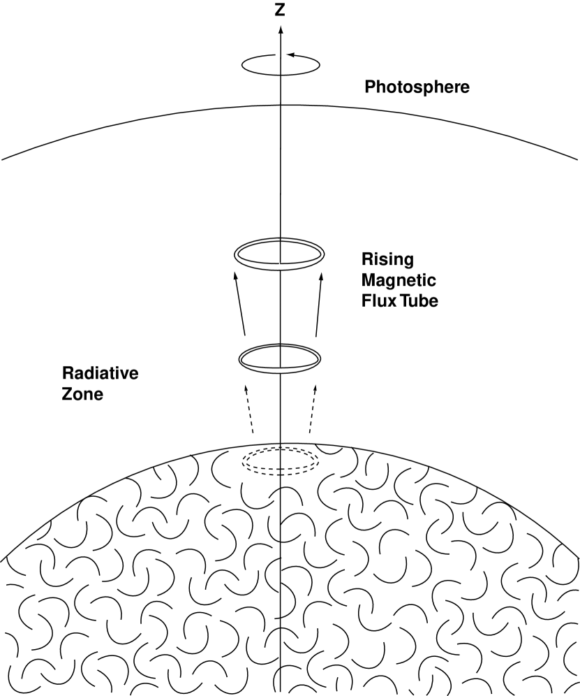
To investigate the buoyant transport of magnetic flux through the radiative interior of a hot star, we consider a spherical star of mass $M_{*}$ and radius $R_{*}$ that contains a central, convective core of mass $M_{c}\ (<M_{*})$ and radius $R_{c}\ (<R_{*})$. The star is assumed to rotate uniformly with angular velocity $\Omega$ around an axis that coincides with the polar axis of a spherical coordinate system $(r,\theta,\phi)$. In the radiative region external to the core, we study the dynamics of an isolated concentration of azimuthally directed magnetic field (i.e., a flux tube) that at any given time takes the form of a circular ring, symmetric about the stellar rotation axis. A similar configuration has been utilized by Choudhuri & Gilman (1987) to examine the influence of rotation on the rise of flux tubes in the solar convection zone. We assume that the cross-sectional profile of the tube is a circle whose radius $a$ is much smaller than either the radius of curvature of the ring or the local scale height of the surrounding, unmagnetized, radiative envelope. The assumed geometry for the rising flux tube is illustrated in Figure 1. These approximations are here used to study the dynamics for the rise of magnetic flux to the stellar surface, and for comparisons of rise times with the main sequence lifetime of the star.

As it is described above, the magnetic ring satisfies the criteria for applicability of the thin flux tube approximation (e.g., Defouw 1976; Spruit 1981), and its internal properties can be reasonably taken to be uniform throughout. The ring is assumed to contain material with mass density $\rho$, so that its total mass is $m=\rho V$, where $V=2\pi r\ {\rm sin}\ \theta\cdot\pi a^{2}$ is the ring volume. It follows from conservation of mass that if a ring with cross-sectional radius $a_{0}$ is released from position $(r_{0},\theta_{0})$ at time $t=0$, its density at some $t\ (>0)$ is

$$\rho=\rho_{0}\left({a_{0}\over a}\right)^{2}\left({r_{0}\ {\rm sin}\ \theta_{0}\over r\ {\rm sin}\ \theta}\right),$$ (1)

where $a$ and $(r,\theta)$ are the tube radius and position at the later time. Likewise, the flux ring is presumed to be untwisted and to contain a toroidal magnetic field of the form ${\bf B}=B\ {\bf e}_{\phi}$ with $B$ a constant. Conservation of magnetic flux then implies that $B$ is related to its initial value $B_{0}$ through the relation

$$B=B_{0}\left({a_{0}\over a}\right)^{2}.$$ (2)

A further consequence of the thin flux tube approximation is that because the time required for a fast magnetosonic wave to transit the tube cross section is short, the total pressure inside the ring can be assumed to instantaneously equilibrate with that of the surrounding stellar material. The quantitative expression of this lateral mechanical equilibrium condition is

$$p_{e}=p+{B^{2}\over 8\pi},$$ (3)

where $p=\rho kT/\mu$ is the gas pressure and the subscript $e$ refers to conditions in the external, field-free medium on the periphery of the tube. Note that by using the ideal gas law for $p$ and $p_{e}$, we are neglecting the radiative component of the total pressure. This omission restricts our analysis to stars less massive than about $10\ M_{\odot}$, for which radiation pressure is a minor contributor to the support of the deep stellar interior. In addition, we assume that the mean molecular weight $\mu$ has the same constant value throughout the star. Our model thus describes conditions within a young, chemically homogeneous, main sequence star; it does not apply at later evolutionary stages when a flux tube that originates in the vicinity of the core-envelope interface may contain chemically processed material.

In a frame of reference that rotates with the stellar angular velocity, the uniform flux ring moves coherently in response to the axisymmetric forces applied to it; that is, each mass element within it has the same velocity

$${\bf u}=u_{r}\ {\bf e}_{r}+u_{\theta}\ {\bf e}_{\theta}+u_{\phi}\ {\bf e}_{\phi}={{\rm d}r\over{\rm d}t}\ {\bf e}_{r}+r\ {{\rm d}\theta\over{\rm d}t}\ {\bf e}_{\theta}+r\ {\rm sin}\ \theta\ {{\rm d}\phi\over{\rm d}t}\ {\bf e}_{\phi}.$$ (4)

The velocity components $(u_{r},u_{\theta},u_{\phi})$ and ring position $(r,\theta)$ can be obtained as functions of time by integration of the ring equation of motion,

$${{\rm d}{\bf u}\over{\rm d}t}+2\ {\bf\Omega}\times{\bf u}=\left({\rho_{e}-\rho\over\rho_{e}+\rho}\right)\left[{GM(r)\over r^{2}}\ {\bf e}_{r}-\Omega^{2}\ r\ ({\rm sin}^{2}\ \theta\ {\bf e}_{r}+{\rm sin}\ \theta\ {\rm cos}\ \theta\ {\bf e}_{\theta})\right]$$

$$\hskip 113.81102pt-{B^{2}\over 4\pi r\ (\rho_{e}+\rho)}\ ({\bf e}_{r}+{\rm cot}~{}\theta\ {\bf e}_{\theta})-C_{D}\left({\rho_{e}\over\rho_{e}+\rho}\right){|{\bf u}_{\bot}|\ {\bf u}_{\bot}\over\pi a},$$ (5)

where $M(r)$ is the internal mass distribution of the star, $C_{D}$ is the drag coefficient, and ${\bf u}_{\bot}\equiv u_{r}\ {\bf e}_{r}+u_{\theta}\ {\bf e}_{\theta}$ is the transverse velocity. The individual components of the inertial and Coriolis terms on the left-hand side of equation (5) have the explicit forms

$$\left({{\rm d}{\bf u}\over{\rm d}t}+2\ {\bf\Omega}\times{\bf u}\right)_{r}={{\rm d}u_{r}\over{\rm d}t}-{(u_{\theta}^{2}+u_{\phi}^{2})\over r}-2\ \Omega\ u_{\phi}\ {\rm sin}\ \theta,\\$$ ()

$$\left({{\rm d}{\bf u}\over{\rm d}t}+2\ {\bf\Omega}\times{\bf u}\right)_{\theta}={{\rm d}u_{\theta}\over{\rm d}t}+{u_{r}u_{\theta}\over r}-{u_{\phi}^{2}\over r}\ {\rm cot}\ \theta-2\ \Omega\ u_{\phi}\ {\rm cos}\ \theta,\\$$ ()

$$\left({{\rm d}{\bf u}\over{\rm d}t}+2\ {\bf\Omega}\times{\bf u}\right)_{\phi}={{\rm d}u_{\phi}\over{\rm d}t}+{u_{r}u_{\phi}\over r}+{u_{\theta}u_{\phi}\over r}\ {\rm cot}\ \theta+2\ \Omega\ (u_{r}\ {\rm sin}\ \theta+u_{\theta}\ {\rm cos}\ \theta).$$ ()

The equation of motion (5) and its many variations have been used to treat the dynamics of buoyant flux tubes in the Sun’s convective envelope by numerous authors, including Choudhuri & Gilman (1987), Choudhuri (1989), Moreno-Insertis, Schüssler, & Ferriz-Mas (1992), Cheng (1992), Fan, Fisher, & DeLuca (1993), Ferriz-Mas & Schüssler (1993, 1994), Fan, Fisher, & McClymont (1994), Caligari, Moreno-Insertis, & Schüssler (1995), and Fan & Fisher (1996), among others. The three terms on the right-hand side of equation (5) describe, respectively, the accelerations produced by: ($i$) the buoyant force, including the effect of the centrifugal reduction of the local gravitational acceleration; ($ii$) the magnetic tension force, arising in response to outward, stretching motion of the ring in the plane perpendicular to the rotation axis of the star; and ($iii$), the aerodynamic drag force, derived from that exerted on a straight, circular cylinder immersed in a steady flow with upstream velocity directed perpendicular to the axis of symmetry (Goldstein 1938). The appearance of the factor $(\rho_{e}+\rho)^{-1}$ rather than $\rho^{-1}$ in the expressions for each of the accelerations reflects the fact that we have made provision for the so-called virtual (or enhanced) inertia of the ring, the hydrodynamical resistance to acceleration experienced by a rigid body that moves through a fluid (see, e.g., Batchelor 1967). Considerable discussion has been devoted to the reasons for including (or not including) this effect in the equation describing the balance of forces acting on a flux tube (see, e.g., Moreno-Insertis, Schüssler, & Ferriz-Mas, 1996; Fan & Fisher 1996, and references therein). As will become clear in subsequent sections, the overall picture of flux ring dynamics that emerges from solutions of equation (5) depends little on the presence or absence of virtual inertia in any of the terms.

The difference between the nature of the energy balance that prevails within the envelope of a massive star and that within the convection zone of the Sun leads to significant differences between the dynamics of flux tubes located in the two regions. The outer portion of the solar interior is adiabatically stratified, a consequence of efficient convective energy transport therein. Because of this, an adiabatic flux tube that is initially buoyant will remain so during the course of its rise toward the surface. Alternatively, the envelope of a hot star is sub-adiabatically stratified, a consequence of the radiative equilibrium conditions that exist throughout it. As a result, the density deficit of an initially buoyant, adiabatic tube will diminish as it rises, causing the upward buoyant acceleration to decrease as well. When adiabatic cooling causes the temperature contrast of the tube relative to its surroundings to attain the value $(T_{e}-T)/T_{e}=(1+\beta)^{-1}$ where $\beta=(8\pi p/B^{2})$, $\rho=\rho_{e}$, and the buoyancy of the tube is reduced to zero.

The discussion of the preceding paragraph indicates that within the envelope of a massive star, the non-adiabatic, radiative interaction between a flux ring and its environment will play an important role in determining the magnitude of the buoyant acceleration the ring experiences, and thus, the time required for it to emerge at the surface of the star (see, e.g., Parker 1975; Moreno-Insertis 1983; Fan & Fisher 1996). In the present model, the heating associated with the diffusion of radiation from the external medium into the tube is described by the thermal energy equation (see Appendix A),

$${{\rm d}S\over{\rm d}t}={32\over 3}\ {(\gamma-1)\ \sigma\ T_{e}^{4}\over\kappa_{e}\ \rho_{e}\ p\ a^{2}}\ {\Delta T\over T_{e}}\equiv q,$$ (7)

where $\Delta T=(T_{e}-T)$, and $S$ is the entropy-like quantity

$$S={\rm ln}\left[\left({p\over p_{0}}\right)\left({\rho_{0}\over\rho}\right)^{\gamma}\right].$$ (8)

In equations (7) and (8), $\gamma$ is the ratio of specific heats, $\sigma$ is the Stefan-Boltzmann constant, and $\kappa_{e}$ is the Rosseland mean opacity in the material surrounding the tube. In the absence of radiative heating (i.e., when $q=0$), equation (7) indicates that $S$ is constant, and the tube behaves adiabatically.

A general question concerning the flux tube approach is how far we can consider the flux tube to be thin in the thermal sense. We assume the heating that arises from the inward diffusion of radiation affects the tube interior uniformly. In reality, the fact that the heating time scale and the tube radius are both finite implies a differential response by the tube to the heat input. In particular, if the time scale for the dynamical adjustment of the tube ($\sim$ the sound crossing time) is much shorter than the diffusion heating time scale, then the temperature in the outermost portion of the tube can become elevated relative to the center, and the resultant enhancement of the buoyant acceleration can cause a deformation of the tube. Unless checked by some additional confining influence (e.g., twisted flux tube fields), this tendency might ultimately lead to the destruction of the flux concentration. While quantitative treatment of this effect is beyond the scope of the present exploratory model calculations, its potential occurence underscores the desirability of performing 2D MHD simulations of flux tubes in a radiative enviroment.

We use the model consisting of equations (1)-(8) to determine the motion of an initially buoyant flux ring in the radiative envelope of a hot star. The distributions of pressure ($p_{e}$), density ($\rho_{e}$), and temperature ($T_{e}$) are taken from a spherical, non-rotating stellar interior model for $M_{*}=9\ M_{\odot}$, kindly calculated for us by S. Jackson. As described in Appendix B, in order to facilitate numerical computations, we have derived an approximate, analytic representation of this model by assuming that $p_{e}$, $\rho_{e}$, and $T_{e}$ are related polytropically. For the purpose of these simulations, the star is assumed to rotate rigidly with a prescribed angular velocity $\Omega$ that is sufficiently slow that departures from sphericity can be neglected.

At time $t=0$, a toroidal flux ring with specified values of the cross-sectional radius $a_{0}$ and plasma beta $\beta_{0}\ (=8\pi p_{0}/B_{0}^{2})$ is released from the outer boundary of the convective core ($r_{0}=R_{c}$) at co-latitude $\theta_{0}$ (latitude $\lambda_{0}$). We suppose that the ring is initially in thermal equilibrium with the ambient stellar material, $T_{0}=T_{e0}$. Application of the mechanical equilibrium condition (3) then yields $p_{0}=p_{e0}\ \beta_{0}/(1+\beta_{0})$ and $\rho_{0}=\rho_{e0}\ \beta_{0}/(1+\beta_{0})$, so that $(\rho_{e0}-\rho_{0})>0$ and the ring is buoyant. The initial field strength $B_{0}$ and Alfvén speed $u_{A0}$ in the ring are given in terms of $\beta_{0}$ and the external properties at the starting position according to $B_{0}=[8\pi p_{e0}/(1+\beta_{0})]^{1/2}$ and $u_{A0}=[2p_{e0}/(\beta_{0}\rho_{e0})]^{1/2}$.

The velocity components ($u_{r},u_{\theta},u_{\phi}$) are obtained as functions of $t$ by numerical integration of the three components of equation (5); the position ($r,\theta$) of the axisymmetric ring follows by integrating the relations ${\rm d}r/{\rm d}t=u_{r}$, ${\rm d}\theta/{\rm d}t=u_{\theta}/r$ given in equation (4). In addition, we simultaneously integrate the thermal energy equation (7) to obtain $S$, which enables us to update the tube properties at each time step. In particular, from the definition given in equation (8), the pressure $p$ within the tube can be expressed as

$$p=p_{0}\ e^{S}\ \left({\rho\over\rho_{0}}\right)^{\gamma}.$$ (9)

Similarly, if equation (1) is rewritten in the form

$$\left({a\over a_{0}}\right)^{2}=\left({\rho_{0}\over\rho}\right)\left({r_{0}\ {\rm sin}\ \theta_{0}\over r\ {\rm sin}\ \theta}\right),$$ (10)

then substitution in equation (2) yields

$$B=B_{0}\left({\rho\over\rho_{0}}\right)\left({r\ {\rm sin}\ \theta\over r_{0}\ {\rm sin}\ \theta_{0}}\right).$$ (11)

This result, together with equation (9), permits the pressure equilibrium condition (3) to be recast as

$$e^{S}\left({\rho\over\rho_{0}}\right)^{\gamma}+{1\over\beta_{0}}\left({r\ {\rm sin}\ \theta\over r_{0}\ {\rm sin}\ \theta_{0}}\right)^{2}\left({\rho\over\rho_{0}}\right)^{2}-\left(1+{1\over\beta_{0}}\right)\left({p_{e}\over p_{e0}}\right)=0,$$ (12)

which is solved to obtain $\rho/\rho_{0}$, given the values of $S$ and $p_{e}$ that prevail at a particular time $t$ and location $(r,\theta)$. Equations (9), (10), and (11) are then used to derive $p$, $a$, and $B$, and $T$ is determined via the relation $T/T_{0}=(p/p_{0})(\rho_{0}/\rho)$.

3 Results

We have used the thin flux tube physical model and solution method outlined in the preceding section to investigate the dynamical behavior of magnetic flux rings with $10^{4}\leq\beta_{0}\leq 10^{7}$ and $10^{-4}\leq(a_{0}/h_{e0})\leq 10^{-2}$, where $h_{e0}$ ($=2.65\times 10^{10}$ cm; see Appendix B) is the pressure scale height in the stellar interior at the starting radius $r_{0}=R_{c}$. The maximum and minimum values adopted for the quantity $\beta_{0}$ correspond to toroidal fields with strengths $B_{0}=1.82\times 10^{5}$ G and $5.77\times 10^{6}$ G, respectively. In the computational results described below, the parameters $\gamma$, $C_{D}$, and $\Omega$ were assigned the values, $\gamma=5/3$, $C_{D}=1$, and $\Omega=5.88\times 10^{-5}$ s^-1, the latter value representing a surface equatorial rotation speed of about 150 km s^-1. We have examined the motion of buoyant flux rings following release from the core boundary at initial latitudes in the range $0^{\circ}\leq\lambda_{0}\leq 45^{\circ}$ (i.e., $\pi/4\leq\theta_{0}\leq\pi/2$). Because the dynamics of rings in the equatorial plane ($\lambda_{0}=0^{\circ}$) differ from those of rings with $\lambda_{0}>0^{\circ}$, we treat the two cases separately in the ensuing discussion.

3.1 Flux Rings in the Equatorial Plane

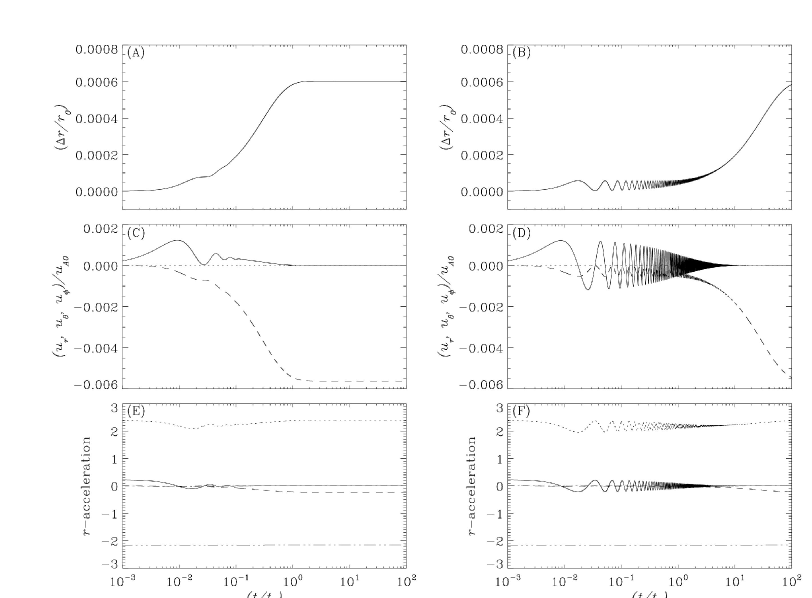
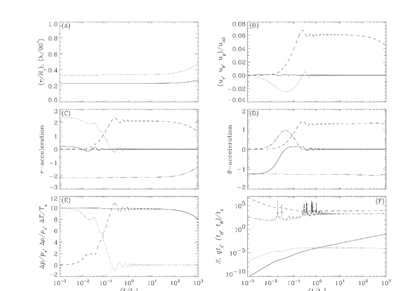
Inspection of the equation of motion (5) reveals that the meridional component of each force acting on a flux ring that is initially at rest (${\bf u}=0$) in the equatorial plane ($\theta=\pi/2$) vanishes identically. The subsequent motion of such a ring therefore remains in this plane, and is governed by just the $r$- and $\phi$-components of equation (5). Some of the properties of configurations of this kind are illustrated in Figures 2 and 3, which contain results pertaining to rings with $\beta_{0}=10^{4}$. The pairs of panels that make up the three rows of Figure 2 show, respectively, the time evolution of: ($i$) the radial position of the ring, $(\Delta r/r_{0})=(r-r_{0})/r_{0}$; ($ii$) the velocity components $(u_{r},u_{\theta},u_{\phi})$ in units of the Alfvén speed $u_{A0}\ (=7.49\times 10^{5}$ cm s^-1) in the ring at $t=0$; and ($iii$), the accelerations produced by each of the forces acting on the ring, in units of $u_{A0}^{2}/R_{*}$. In each panel, time is measured in units of the Alfvén time $t_{A}$, defined as $t_{A}\equiv R_{*}/u_{A0}\ (=3.42\times 10^{5}$ s $\approx 4$ days).

The dynamical evolution of a flux ring with initial cross-sectional radius $a_{0}=10^{-4}\ h_{e0}$ is shown in panels (A), (C), and (E) of Figure 2. Note that in this case, the outward expansion of the ring ceases after $t\approx t_{A}$, its radial position remaining fixed at later times. In the course of evolving toward this apparent equilibrium configuration, the ring experiences a brief, initial period of accelerated motion in the $+{\bf e}_{r}$-direction, followed by radial deceleration to a state of rest in which $u_{r}=0$ but $u_{\phi}\neq 0$. Examination of the ring force balance indicates that the initial expansion is driven (as expected) by buoyancy, while being opposed by the slightly smaller, inward-directed, magnetic tension force. The aerodynamic drag force, although small in magnitude, contributes to the damping of the oscillatory motions that are induced by the interplay between the larger buoyant and magnetic forces.

The flux ring is assumed to corotate with the stellar interior at $t=0$, so that its initial azimuthal velocity is $u_{\phi 0}=0$ in the reference frame that rotates with angular velocity $\Omega$. For $t>0$, the azimuthal motion of the ring is such that the angular momentum of the material contained within it is conserved. The buoyancy-driven increase in the radial position of the ring is therefore accompanied by a decrease in the rotation rate of the ring material. Hence, in the frame of reference that corotates with the star, the azimuthal velocity of the ring is in the $-{\bf e}_{\phi}$-direction, as can be seen in panel (C). According to equation (6$a$), this azimuthal motion produces an inward-directed Coriolis force that grows with increasing $\Delta r$ until its magnitude, combined with that of the magnetic tension force, is sufficient to balance the buoyant force and prevent further radial expansion of the ring. A similar behavior has been observed in connection with models of equatorial magnetic flux rings located in the radiative layers just below the base of the solar convection zone (Moreno-Insertis, Schüssler, and Ferriz-Mas 1992; Ferriz-Mas 1996).

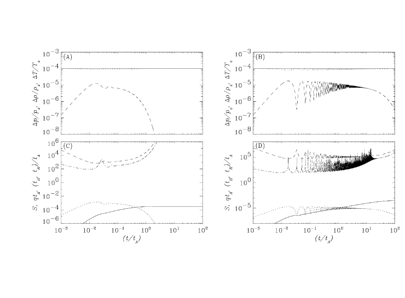
In panels (A) and (C) of Figure 3, we show how the thermodynamic state of a ring with $\beta_{0}=10^{4}$ and $a_{0}=10^{-4}\ h_{e0}$ evolves over time. Panel (A) shows the normalized differences between the pressure, density, and temperature in the tube and in the material surrounding it (i.e., $\Delta p/p_{e}$, $\Delta\rho/\rho_{e}$, and $\Delta T/T_{e}$, respectively, where for any quantity $Q$, $\Delta Q\equiv Q_{e}-Q$) as functions of time. Beginning from a state in which $T_{0}=T_{e0}$, the ring cools slightly relative to its surroundings during the earliest and most rapid portion of its limited buoyant ascent. As its outward progress stalls, radiative heating acts to restore the condition of thermal equilibrium between the ring and its external environment. In panel (C), we display the time evolution of the quantities $S$ and $q$ (see equations [7] and [8]), along with the corresponding histories of the instantaneous heating and rise times, defined as $t_{H}\equiv q^{-1}$ (see Appendix A) and $t_{R}\equiv|h_{e}/u_{r}|$, respectively. Note that $S$ increases as the tube is radiatively heated, and approaches a constant value as $u_{r}\rightarrow 0$, $T\rightarrow T_{e}$, and both $t_{H}$ and $t_{R}$ become large.

To further explore the nature of the equilibrium seen in Figures 2 and 3 for flux rings in the equatorial plane, we write the $\phi$-component of the equation of motion (5) in the form

$$r{{\rm d}u_{\phi}\over{\rm d}t}+u_{r}u_{\phi}+2u_{r}\Omega r={{\rm d}\over{\rm d}t}\left(ru_{\phi}+\Omega r^{2}\right)=0,$$ (13)

where we have assumed $u_{\theta}=0$ for $\theta=\pi/2$, and have used the fact that $u_{r}={\rm d}r/{\rm d}t$. Equation (13) implies that the specific angular momentum $(ru_{\phi}+\Omega r^{2})$ has a constant value which, after recalling the initial condition $u_{\phi 0}=0$, is readily established to be $\Omega r_{0}^{2}$. This quantity can then be used to evaluate the azimuthal velocity component of the ring, yielding the result

$$u_{\phi}=\left({\Omega r_{0}^{2}\over r}\right)-\Omega r.$$ (14)

Similar considerations applied to the $r$-component of equation (5) lead to the equilibrium condition

$$\left({\rho_{e}-\rho\over\rho_{e}+\rho}\right)\left[{GM(r)\over r^{2}}-\Omega^{2}\ r\right]+{u_{\phi}^{2}\over r}+2\ \Omega\ u_{\phi}-{B^{2}\over 4\pi r\ (\rho_{e}+\rho)}=0,$$ (15)

where we have set $u_{r}=({\rm d}u_{r}/{\rm d}t)=0$. Equation (15) expresses the fact that the radial equilibrium is characterized by a balance between the outward-directed buoyancy and centrifugal forces and the inward-directed Coriolis and magnetic tension forces. Making the substitution $(r/r_{0})=1+(\Delta r/r_{0})$ and retaining only the lowest order terms in $(\Delta r/r_{0})$ ($\ll 1$), we obtain

$${\Delta r\over r_{0}}\approx{1\over 8(\Omega r_{0})^{2}}\left({GM_{c}\over\beta_{0}r_{0}}-u_{A0}^{2}\right)={1\over 8\beta_{0}(\Omega r_{0})^{2}}\left({GM_{c}\over r_{0}}-{2p_{e0}\over\rho_{e0}}\right),$$ (16)

where equation (14) and the approximation $\rho_{e}\approx\rho\ [1+(1/\beta_{0})]$ have been used in simplifying equation (15).

As is evident from equation (16), for a given stellar model, the equilibrium position of an equatorial flux ring depends only on the value of the parameter $\beta_{0}$; in the case of the present model, $(\Delta r/r_{0})\approx 6\times 10^{-4}\ (\beta_{0}/10^{4})^{-1}$. This dependence has been confirmed by examination of solutions corresponding to a variety of input parameter values, including the particular example shown in panels (B), (D), and (F) of Figure 2, and in panels (B) and (D) of Figure 3. For this solution, $\beta_{0}=10^{4}$ as in the case of the ring considered above, but $a_{0}=10^{-3}\ h_{e0}$. Because this initial cross-sectional radius is a factor of 10 larger than the previous value, the radiative heating rate $q$ and the acceleration produced by the aerodynamic drag force are smaller by factors of 100 and 10, respectively (see equations [5] and [7]). As can be seen in the relevant portions of Figures 2 and 3, a consequence of these reductions is that the ring is subject to vigorous buoyancy oscillations in the radial direction. Oscillations of a similar kind in toroidal flux tubes inside non-rotating stars have been studied by Spruit & van Ballegooijen (1982), and inside rotating stars by van Ballegooijen (1983), Moreno-Insertis, Schüssler, & Ferriz-Mas (1992), and Ferriz-Mas & Schüssler (1993). In the present example, the enhanced tendency toward oscillatory motion is directly attributable to modifications in the buoyant acceleration of the ring; these changes are themselves a result of the altered thermodynamic state of the ring material, produced by the diminished rate of radiative heating. The build-up in the magnitude of the Coriolis force, together with the action of the drag force, cause the amplitude of these oscillations to decrease over time, leaving the ring in the same equilibrium configuration that obtained in the case of the $a_{0}=10^{-4}\ h_{e0}$ ring studied above.

These results suggest that the equilibrium of a flux ring located in the equatorial plane is stable with respect to small amplitude, radial displacements from the position given by equation (16). This conjecture has been verified by a series of numerical experiments in which an additional, radially directed force of specified amplitude is applied to the ring for a brief time interval after it has assumed its equilibrium position. In all cases, the ring is initially displaced in radius, but is quickly restored to its original location following cessation of the imposed forcing. Such behavior is not observed in response to the application of latitudinal forcing of the same type. In all of these cases, a small displacement out of the equatorial plane is accompanied by the development of a $\theta$-component of the magnetic tension force that accelerates the ring toward the pole. This is similar to the dynamical evolution of the so-called poleward-slip instability of equatorial flux rings in the radiative layers beneath the solar convection zone (see, e.g., Moreno-Insertis, Schüssler, & Ferriz-Mas 1992, and references therein). For the conditions considered in the present paper, the perturbed force balance is such that a ring initially contained within the equatorial plane moves over time to higher latitudes and larger radii. Once out of the equatorial plane, the dynamics of such a ring is found to be identical to that of one with $\theta_{0}<\pi/2$, and is discussed in §3.2 below.

3.2 Flux Rings Outside of the Equatorial Plane

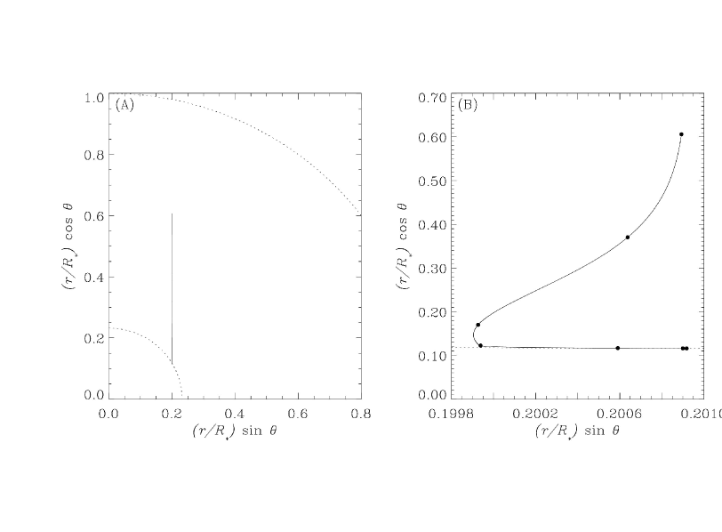
We now consider the motion of toroidal magnetic flux tubes having initial positions $r_{0}=R_{c}$ with $0<\theta_{0}<\pi/2$. We focus on the properties of rings with $\theta_{0}=\pi/3$ (i.e., initial latitude $\lambda_{0}=30^{\circ}$) since the behavior in this case is representative of that displayed by all rings having starting locations along the core-envelope interface, out of the equatorial plane. In Figure 4, we show the trajectory that a ring with $\beta_{0}=10^{4}$ and $a_{0}=10^{-4}\ h_{e0}$ follows during the time interval between its release and $t=10^{3}\ t_{A}\approx 10.85$ years. As can be seen in panel (A), the edge of the ring traces a path that is nearly parallel to the stellar rotation axis over this period, extending from $r_{0}=0.232\ R_{*}$ and $\lambda_{0}=30^{\circ}$ to $r=0.64\ R_{*}$ and $\lambda=72^{\circ}$. In panel (B), we have magnified the horizontal scale in order to make the meridional motion of the ring more apparent. There it can be seen that for a time $t\approx 5\ t_{A}$ after the start of the calculation, the distance $r\ {\rm sin}\ \theta$ of the ring from the stellar rotation axis decreases as the ring moves toward higher latitudes along the periphery of the convective core. At later times, this moment arm length approaches its initial size, while the height $r\ {\rm cos}\ \theta$ of the ring above the equatorial plane steadily increases.

Additional information pertaining to the evolving dynamical and thermodynamical properties of the flux ring under consideration is presented in Figure 5. Inspection of panels (A) and (B) reveals that after a brief, initial period of dynamical readjustment, the ring moves continuously in the direction of higher latitudes (i.e., the $-{\bf e}_{\theta}$-direction) and larger radii. This is unlike the behavior of rings with $\lambda_{0}=0^{\circ}$ which, in the absence of suitable perturbations, do not depart from the equatorial plane as they evolve toward a final equilibrium state with $u_{r}=u_{\theta}=0$ (see §3.1). In the present case, although its upward progress slows considerably at later times, the ring never attains an equilibrium in which the forces acting in the ${\bf e}_{r}$- and ${\bf e}_{\theta}$-directions balance to produce a state of rest.

Details concerning the radial and meridional dynamics of the flux ring are provided in panels (C) and (D) of Figure 5. When the ring is released at $t=0$, it experiences a net radial acceleration that is $>0$, resulting from the fact that the outward, buoyant force is larger than the inward, radial component of the tension force. In the ${\bf e}_{\theta}$-direction, the tension force is initially unopposed by any other force components, leading to a net meridional acceleration that is $<0$. The ring is therefore pulled toward the pole, and the horizontal distance $r\ {\rm sin}\ \theta$ between it and the rotation axis decreases (see Figure 4). This change in position has an important consequence for the subsequent motion of the ring. In order to conserve angular momentum, the azimuthal velocity $u_{\phi}$ increases as the moment arm of the ring material becomes smaller (see panel [B]). Associated with this spin-up are substantial increases in the magnitudes of the $r$- and $\theta$-components of the Coriolis force, both of which exert considerable influence over the dynamical evolution of the ring.

Using a procedure similar to that adopted in the case of an equatorial flux ring, the azimuthal component of the equation of motion (5) for a ring at higher latitudes can, after some manipulation, be written as

$${{\rm d}\over{\rm d}t}\left(r\ {\rm sin}\ \theta\ u_{\phi}+\Omega r^{2}\ {\rm sin}^{2}\ \theta\right)=0,$$ (17)

from which it immediately follows that

$$u_{\phi}=\left({\Omega r_{0}^{2}\ {\rm sin}^{2}\ \theta_{0}\over r\ {\rm sin}\ \theta}\right)-\Omega r\ {\rm sin}\ \theta.$$ (18)

Note that in this case, because the initial radial and meridional motion of the ring corresponds to decreasing $r\ {\rm sin}\ \theta$, the sense of the azimuthal motion is such that $u_{\phi}>0$. Hence, the accelerations produced by the Coriolis force in the ${\bf e}_{r}$- and ${\bf e}_{\theta}$-directions, $2\ \Omega\ u_{\phi}\ {\rm sin}\ \theta$ and $2\ \Omega\ u_{\phi}\ {\rm cos}\ \theta$, respectively, are both $>0$. As a result, the tension-induced, poleward movement of the ring at early times begins to slow when the sum of the $\theta$-components of the Coriolis and drag forces becomes large enough to change the sign of the net meridional acceleration, making it $>0$. Likewise, the acceleration supplied by buoyancy and the radial Coriolis force component causes $u_{r}$ to grow until $u_{r}=-u_{\theta}\ {\rm cot}\ \theta$, at which point contraction of the ring toward the rotation axis ceases; at later times, $u_{r}>-u_{\theta}\ {\rm cot}\ \theta$, and the ring expands. The resulting increase in $r\ {\rm sin}\ \theta$ leads to a gradual reduction in $u_{\phi}$, and leaves the ring in a state of near balance between the Coriolis and tension forces in both the ${\bf e}_{r}$- and ${\bf e}_{\theta}$-directions.

The lack of equilibria for flux rings that originate at latitudes $\lambda_{0}>0^{\circ}$ can be understood by examining the $r$- and $\theta$-components of the equation of motion (5). Assuming that a stationary state with $u_{r}=u_{\theta}=0$ exists, the $r$-component can be written in a form reminiscent of the equilibrium condition (15) for flux rings in the equatorial plane,

$$\left({\rho_{e}-\rho\over\rho_{e}+\rho}\right)\left[{GM(r)\over r^{2}}-\Omega^{2}\ r\ {\rm sin}^{2}\ \theta\right]+{u_{\phi}^{2}\over r}+2\ \Omega\ u_{\phi}\ {\rm sin}\ \theta-{B^{2}\over 4\pi r\ (\rho_{e}+\rho)}=0,$$ (19)

while the $\theta$-component becomes

$$-\left({\rho_{e}-\rho\over\rho_{e}+\rho}\right)\ \Omega^{2}\ r\ {\rm sin}^{2}\ \theta+{u_{\phi}^{2}\over r}+2\ \Omega\ u_{\phi}\ {\rm sin}\ \theta+{B^{2}\over 4\pi r\ (\rho_{e}+\rho)}=0.$$ (20)

Note that were it not for the appearance of the gravitational acceleration in the radial component, equations (19) and (20) would be identical. This correspondence implies that the conditions for force balance in the ${\bf e}_{r}$- and ${\bf e}_{\theta}$-directions can be simultaneously satisfied only if $\rho=\rho_{e}$. However, as can be seen in panel (E) of Figure 5, $\rho<\rho_{e}$ throughout the time interval covered by the calculation, indicating that a stationary equilibrium is not possible in this particular case.

In general, all magnetic flux rings with $\lambda_{0}>0^{\circ}$ remain slightly cooler and less dense than the surrounding material during most of their ascent, a consequence (in part) of the total pressure balance condition given by equation (3). On the basis of equations (19) and (20) then, stationary equilibria are ruled out for toroidal flux tubes of this kind. Because $T<T_{e}$ (see panel [E] of Figure 5), a given tube is heated by the radiation that diffuses into it from the external medium. In response to this heating and in order to comply with the pressure equilibrium condition, the tube expands, becoming less dense as it does so. Buoyancy then carries the tube outward to a somewhat larger radius. Hence, apart from a brief period at the start of the motion when the buoyant acceleration is established by the initial conditions, the rate of rise of the tube is controlled by the rate at which it is radiatively heated. This behavior is evident in panel (F) of Figure 5, wherein it can be seen that for much of the time interval depicted, the heating and rise times vary in concert. Such a situation is in contrast to the dynamical and thermodynamical evolution observed previously for flux rings in the equatorial plane. The stationary equilibrium of an equatorial flux ring is characterized by $T=T_{e}$, a vanishing radiative heating rate, and a balance between buoyancy and the sum of the Coriolis and tension forces (see Figures [2] and [3]).

The considerations of the preceding paragraph can be used to derive an approximate expression for the radial rise speed of a buoyant flux ring. Interpreting the derivative on the left-hand side of equation (7) as $({\rm d}S/{\rm d}t)=u_{r}({\rm d}S/{\rm d}r)$, the sought-after component of the tube velocity is

$$u_{r}={q\over({\rm d}S/{\rm d}r)},$$ (21)

where $q$ and $S$ are defined in equations (7) and (8). To evaluate $({\rm d}S/{\rm d}r)$, we assume that since $\beta\gg 1$, $p\approx p_{e}$ and $\rho\approx\rho_{e}$; then,

$$S\approx{\rm ln}\left[{p_{e0}\over p_{0}}\left({\rho_{0}\over\rho_{e0}}\right)^{\gamma}\right]+\left({\alpha-\gamma\over\alpha}\right){\rm ln}\left({p_{e}\over p_{e0}}\right),$$ (22)

where we have made use of the polytrope relation in the form $(\rho_{e}/\rho_{e0})=(p_{e}/p_{e0})^{1/\alpha}$. Thus,

$${{\rm d}S\over{\rm d}r}\approx\left({\alpha-\gamma\over\alpha}\right){{\rm d\ ln}\ p_{e}\over{\rm d}r}=\left({\gamma-\alpha\over\alpha}\right){1\over h_{e}},$$ (23)

and

$$u_{r}\approx\left({\alpha\over\gamma-\alpha}\right)q\ h_{e},$$ (24)

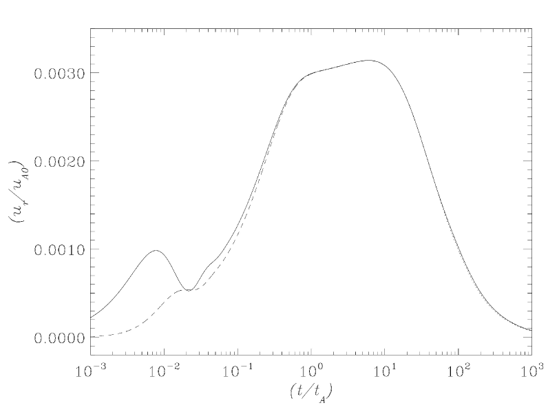
where $h_{e}=p_{e}/(\rho_{e}g)$ is the pressure scale height. In Figure 6, we compare the approximation given in equation (24) with the radial velocity component obtained by numerical solution of the full equation of motion for $\beta_{0}=10^{4}$, $a_{0}=10^{-4}\ h_{e0}$, and $\lambda_{0}=30^{\circ}$. At times later than $t\approx t_{A}$, the two results are indistinguishable, indicating that the rate of ascent is indeed regulated by the radiative heating of the ring. In fact, using the definitions of the heating and rise time scales, equation (24) implies that $t_{R}\propto t_{H}$, in accordance with the behavior seen in panel (F) of Figure 5.

Figures 7 and 8 contain a summary of results from the simulated rise of a toroidal magnetic flux tube released at latitude $\lambda_{0}=30^{\circ}$ with $\beta_{0}=10^{4}$ and $a_{0}=10^{-3}\ h_{e0}$. As was discussed in §3.1, the larger cross-sectional radius of this tube implies that the deceleration due to aerodynamic drag ($\propto a^{-1}$) and the radiative heating rate ($\propto a^{-2}$) are both reduced from the magnitudes these quantities have when $a_{0}=10^{-4}\ h_{e0}$. Similar to the equatorial flux rings that were the subject of that section, in the present case, these reductions are responsible for engendering oscillatory motion of the tube during the early stages of its ascent toward the surface. Such behavior can be seen in Figure 7, in which (as in Figure 4) two views of the path taken by the rising tube are given. In panel (A), it is apparent that the larger tube is less buoyant; during the time interval $\Delta t=10^{3}\ t_{A}$ between the first and last points on the trajectory, the radial position of the ring only increases from $r_{0}=0.232\ R_{*}$ to $r=0.275\ R_{*}$. On the expanded scale of panel (B), it is seen that for a time $\approx 0.25\ t_{A}$ following the start of the calculation, the ring moves steadily toward the pole, and thereafter executes latitudinal oscillations that decrease in amplitude as the distance of the ring from the equatorial plane increases.

Inspection of the relevant panels of Figure 8 indicates that as in the case of the $a_{0}=10^{-4}\ h_{e0}$ tube considered earlier in this section, the initial poleward motion is driven by the magnetic tension force. However, in the present case, the tube acquires a higher meridional velocity and approaches closer to the rotation axis during this movement, a consequence of the fact that the deceleration due to drag is smaller. Also, the change in volume arising from the decrease in $r\ {\rm sin}\ \theta$, together with the diminshed efficiency of radiative heating, are sufficient to ultimately make $\Delta\rho<0$, and to thereby change the sign of the buoyant acceleration (see panels [C] and [E]). Note that the the spin-up associated with the overall contraction of the ring causes both components of the Coriolis acceleration to increase substantially; the oscillatory behavior seen in Figure 7 results from the interplay between this acceleration and that produced by the magnetic tension force.

3.3 Rise Times

A primary focus of the present investigation is the buoyant transport of magnetic flux from the assumed site of its generation in the convective core to the stellar surface. Of particular interest is an estimate of the time required for this transport to take place. From the definition of $u_{r}$ given in equation (4), it follows that

$$t_{r}(r)=\int\limits^{r}_{r_{0}}{{\rm d}r\over u_{r}},$$ (25)

is the time it takes a flux ring to travel outward from $r_{0}$ to any radius $r>r_{0}$.

We have computed $t_{r}(r)$ for toroidal flux tubes having the properties listed in Table 1. For each case, the radial component of the tube velocity was determined by numerical integration of the full equation of motion (5) for a time interval $0\leq t\leq t_{1}$, where the value of $t_{1}$ for a given solution was chosen to be between $10^{3}\ t_{A}$ and $3\times 10^{4}\ t_{A}$, depending upon the magnitude of $u_{r}$ for that solution. For $t>t_{1}$, $u_{r}$ was evaluated using an analytic approximation to equation (24), derived in the following way.

Table 1: Properties of Magnetic Flux Ring Solutions

Number	$\beta_{0}$	$a_{0}/h_{e0}$	$C_{D}$	$B_{0}$	$t_{r}(0.96\ R_{*})$
				(G)	(years)
1	$10^{4}$	$10^{-4.0}$	1	$5.77\times 10^{6}$	$1.3010\times 10^{5}$
2	$10^{4}$	$10^{-3.0}$	1	$5.77\times 10^{6}$	$1.3225\times 10^{7}$
3	$10^{4}$	$10^{-4.0}$	0	$5.77\times 10^{6}$	$1.3009\times 10^{5}$
4	$10^{4}$	$10^{-4.0}$	1	$5.77\times 10^{6}$	$1.3020\times 10^{5}$
5	$10^{5}$	$10^{-4.0}$	1	$1.82\times 10^{6}$	$1.3011\times 10^{6}$
6	$10^{5}$	$10^{-3.5}$	1	$1.82\times 10^{6}$	$1.3024\times 10^{7}$
7	$10^{5}$	$10^{-3.0}$	1	$1.82\times 10^{6}$	$1.3037\times 10^{8}$
8	$10^{6}$	$10^{-4.0}$	1	$5.77\times 10^{5}$	$1.3011\times 10^{7}$
9	$10^{6}$	$10^{-3.0}$	0	$5.77\times 10^{5}$	$1.3013\times 10^{9}$
10	$10^{7}$	$10^{-4.0}$	1	$1.82\times 10^{5}$	$1.3011\times 10^{8}$

According to equation (24), $u_{r}\propto q\ h_{e}$ at times late enough that any transient behavior stemming from the adjustment of the tube to the imposed initial conditions has disappeared. The heating rate $q$ depends directly on the temperature difference $\Delta T$ between the tube and its surroundings; using the pressure equilibrium condition (3), it can be shown that $(\Delta T/T_{e})\approx B^{2}/(8\pi p_{e})$, assuming $\rho\approx\rho_{e}$. Inserting this result in the definition of $q$ (see Appendix A), we find that the dependence of $u_{r}$ on the physical properties of the tube and the external medium is given by (see also Gurm & Wentzel 1967; Parker 1975)

$$u_{r}\approx{32\over 3}\left[{\alpha\ (\gamma-1)\over\gamma-\alpha}\right]\left({\sigma\ T_{e}^{4}\over\kappa_{e}\ \rho_{e}^{2}\ g}\right)\left({B^{2}\over 8\pi\ p\ a^{2}}\right).$$ (26)

To further simplify this expression, note that as evidenced by Figures 4 and 7, much of the ascent toward the surface takes place with $r\ {\rm sin}\ \theta\approx$ constant (i.e., $u_{r}\approx-u_{\theta}\ {\rm cot}\ \theta$). Therefore, from equations (1) and (2), $\rho\ (\approx\rho_{e})\ \propto a^{-2}$ and $B\propto a^{-2}\propto\rho_{e}$, so that $u_{r}$ varies as

$$u_{r}\propto{T_{e}^{3}\over\kappa_{e}\ g},$$ (27)

where we have approximated $p\ a^{2}\propto T\approx T_{e}$. To illustrate the validity of equation (27), we have evaluated the constant of proportionality using the properties of solution 1 (see Table 1) at the time $t=50\ t_{A}$. The rise speed so-derived is shown as a function of time for $t\geq 50\ t_{A}$ by the dotted line in Figure 6.

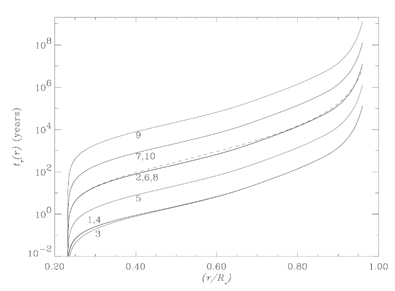
The results of our rise time computations are depicted in graphical form in Figure 9. There we show the time $t_{r}(r)$ required to reach a given radius $r$ within the interval $0.232\ R_{*}\leq r\leq 0.960\ R_{*}$, for each of the solutions listed in Table 1. It is apparent that rings with smaller values of $\beta_{0}$ and $a_{0}$ generally traverse the radiative envelope in less time than do rings that are less strongly magnetized and have larger cross-sectional radii (see also Moss 1989). Based on the discussion of the preceding subsection, rings having smaller values of $\beta_{0}$ and $a_{0}$ are initially more buoyant, and are more likely to remain so because of the comparatively shorter time it takes to heat them by inward diffusion of radiation. With the exception of the rings corresponding to solutions 7, 9, and 10, the time needed to arrive at the stellar surface is less than the estimated main sequence lifetime of the 9 $M_{\odot}$ model, $t_{MS}\approx 10^{10}\ (M_{*}/M_{\odot})(L_{\odot}/L_{*})\approx 2.4\times 10^{7}$ years. However, note that even the more slowly rising tubes of solutions 7, 9, and 10 attain radii in the range (0.92-0.95) $R_{*}$ within a time $<t_{MS}$. In fact, all of the solutions shown in Figure 9 spend more time crossing the outer 10% of the stellar radius than they do traveling from $r=r_{0}$ to $r=0.9\ R_{*}$. From equation (27), it can be seen that since $T_{e}$ decreases and $\kappa_{e}$ increases as $r$ approaches $R_{*}$ in the outer envelope, $u_{r}$ becomes small and the rise time increases accordingly.

Examination of Table 1 and Figure 9 also reveals that the omission of virtual inertia and aerodynamic drag from the equation of motion has little impact on ring dynamics and rise times (see solutions 1, 3, and 4). This is because the flux rings considered herein do not experience significant, impulsive accelerations, and never achieve large rise speeds for prolonged periods of time. Instead, most of the ascent takes place at the slow, quasi-steady rate given by equation (24) (or the approximation [25]). This behavior accounts for another notable characteristic of the results shown in Figure 9, namely, that the rise time profiles of several solutions are nearly identical to one another. From equation (26), it is readily seen that the dependence of the rise speed on the intrinsic properties of a given flux ring is $u_{r}\propto(a^{2}\ \beta)^{-1}$. Consideration of the entries in Table 1 indicates that, as expected, solutions having a common profile of $t_{r}(r)$ in Figure 9 are characterized by the same value of the parameter combination $(a_{0}^{2}\ \beta_{0})^{-1}$.

Finally, we note that with the preceding developments, it is possible to derive an approximate expression for the rise time $t_{r}(r)$. To do this, we first use the equation of hydrostatic equilibrium in the form ${\rm d}\rho_{e}/{\rm d}r=-(g\ \rho_{e})/c_{e}^{2}$, where $c_{e}$ is the external sound speed, to convert the integration variable in equation (25) from $r$ to $\rho_{e}$; this procedure yields

$$t_{r}(r)=-\int\limits^{\rho_{e}}_{\rho_{e0}}{\rm d}\rho_{e}\ \left({c_{e}^{2}\over\rho_{e}\ g\ u_{r}}\right)\approx-\left({c_{e0}^{2}\over\rho_{e0}\ g_{0}\ u_{r0}}\right)\int\limits^{\rho_{e}}_{\rho_{e0}}{\rm d}\rho_{e}\ \left({\rho_{e}\over\rho_{e0}}\right)^{(\alpha-2)}\left({T_{e0}\over T_{e}}\right)^{3}\left({\kappa_{e}\over\kappa_{e0}}\right).$$ (28)

To obtain the second, approximate equality in equation (26), we have replaced $u_{r}$ by the scaling relation (27) and used the fact that $c_{e}^{2}=c_{e0}^{2}\ (\rho_{e}/\rho_{e0})^{(\alpha-1)}$ where $c_{e0}^{2}=(\alpha\ p_{e0}/\rho_{e0})$. The integrand in equation (26) can be simplified by assuming that the opacity follows Kramer’s law, $\kappa_{e}\propto\rho_{e}T_{e}^{-3.5}$. This assumption, together with the polytrope relation $T_{e}\propto\rho_{e}^{(\alpha-1)}$ (see Appendix B), allows us to express the integrand as a function of $\rho_{e}$ only; performing the integration we obtain

$$t_{r}(r)=\left({2\over 11\ \alpha-13}\right)\ \left({c_{e0}^{2}\over g_{0}\ u_{r0}}\right)\ \left[\left({\rho_{e}\over\rho_{e0}}\right)^{-{(11\alpha-13)\over 2}}-1\right].$$ (29)

If $u_{r0}$ is determined by evaluating equation (26) at $r_{0}$, the rise time estimate (27) becomes

$$t_{r}(r)=3.0835\times 10^{3}\ \left[\left({a_{0}\over h_{e0}}\right)^{2}\ \beta_{0}\right]\ \left[\left({\rho_{e}\over\rho_{e0}}\right)^{0.9349}-1\right]\ {\rm years},$$ (30)

where the interior model of Appendix B has been used to fix the values of all physical quantities at the core-envelope interface. As an example, the  dashed line in Figure 9 represents the rise time profile obtained from equation (30) for $[(a_{0}/h_{e0})^{2}\ \beta_{0}]=10^{-2}$

4 Conclusions and Discussion

The foregoing examination of the physics of magnetic flux rings in the radiative envelope of a uniformly rotating hot star has revealed a range of possible dynamical behaviors, and has enabled us to estimate the efficiency of buoyancy as a means of transporting dynamo-generated fields from the core to the surface. Rings located in the equatorial plane can attain a stationary equilibrium in which $u_{r}=0,\ u_{\phi}\neq 0$, and the combined Coriolis and tension forces balance buoyancy. This state is stable against infinitesimal displacements of the ring in the radial direction, but unstable when the perturbations are meridionally directed, causing the ring position to shift from latitude $0^{\circ}$. Apart from transient episodes of oscillatory behavior at the outset of their motion, rings released from latitudes other than $0^{\circ}$ move to larger radii along paths that are very nearly parallel to the stellar rotation axis. During most of the ascent, the rate of rise of such a ring is controlled by the rate at which it is radiatively heated, with a near balance prevailing between the accelerations produced by the Coriolis and magnetic tension forces in the $r$- and $\theta$-directions.

Strongly magnetized rings with smaller cross-sectional radii experience larger initial buoyant accelerations and have shorter radiative heating time scales. As a result, they attain higher rise speeds and require less time to traverse the envelope than do rings with weaker fields and/or larger cross-sectional radii (see also Moss 1989). A majority of the ring models enumerated in Table 1 reach the stellar surface in a time that is less than the main sequence lifetime of the 9 $M_{\odot}$ star, the only exceptions being solutions with large values of $\beta_{0}$ and/or $a_{0}$. If the field strengths and flux tube sizes considered herein are realistic, this result suggests that the field produced by a core dynamo could manifest itself in the surface layers of a hot star at a relatively early stage of main sequence evolution. In light of the discussion of §3, the strength of the field in a buoyant flux ring that reaches the photosphere of the 9 $M_{\odot}$ stellar model is estimated to be $B_{*}\approx B_{0}\ (\rho_{e*}/\rho_{e0})\approx 9.44\ (\beta_{0}/10^{4})^{-1/2}$ G.

The preceding conclusions are drawn from results obtained using a simple model for a thin, isolated, untwisted flux ring immersed in a non-evolving, rigidly rotating stellar interior. Given the exploratory character of this investigation, a more detailed treatment of flux tube structure and dynamics is neither warranted nor practical. However, several potentially important effects that have been neglected in the present analysis can be included within the context of the basic model of §2. Among these are large-scale internal circulatory flows, the development (over time) of gradients in composition and angular velocity, the influence of radiation pressure on tubes inside more massive stars, mass loss, and the consequences of magnetic interference with radiative energy transport (e.g., thermal shadows and small-scale flows; Parker 1984).

Of the effects noted above, rotationally driven, meridional circulation may have the most significant impact on the results described in §3. As noted in that section, each of the ring models listed in Table 1 spends considerably more time traveling through the thin shell $0.90\ R_{*}\leq r\leq 0.96\ R_{*}$ than in ascending from the starting radius to $r=0.90\ R_{*}$ (see Figure 9). In solution 1, for example, the former displacement requires approximately $1.29\times 10^{5}$ years, while the latter occurs in only $1.38\times 10^{3}$ years, a difference in travel time of nearly a factor of 100. We point out that the inclusion of meridional circulation may decrease the time needed to transport magnetic flux through the layers just below the photosphere. Estimates of the circulation speed inside upper main sequence stars suggest that while such flows proceed quite slowly at great depth, they can become fast in the lower-density region near the surface (see, e.g., Kippenhahn & Weigert 1994). Hence, flux tube advection by a circulatory flow may act to supplement buoyant transport in the outermost portion of the stellar interior, thereby shortening the time between the production of fields in the core and their emergence in the atmosphere. The combined effects of buoyancy and advection will be investigated in the next paper of this series.

Appendix A Derivation of the Ring Energy Equation

To derive the energy equation for a thin, axisymmetric magnetic flux ring, we begin with the first law of thermodynamics, written in the form,

$${{\rm d}{\cal E}\over{\rm d}t}+p\ {{\rm d}\over{\rm d}t}\left({1\over\rho}\right)={{\rm d}{\cal Q}\over{\rm d}t},$$ (A1)

where ${\cal E}=(p/\rho)/(\gamma-1)$ is the specific internal energy of the gas, and $({\rm d}{\cal Q}/{\rm d}t)$ is the rate at which heat is input, per unit mass of ring material. Let $F_{e}$ be the radiative flux at the surface of the ring; in the case of interest to us here, $T<T_{e}$, and this flux is directed into the ring from the external medium. We assume that the ring is sufficiently opaque that all of the flux incident upon it is thermalized within it. For a ring of mass $M$, the specific radiative heating rate is then

$${{\rm d}{\cal Q}\over{\rm d}t}={A\ F_{e}\over M}={2\ F_{e}\over\rho\ a},$$ (A2)

where $A=2\pi a\cdot 2\pi r\ {\rm sin}\ \theta$ is the surface area of the ring. If ${\bf\nabla}T_{e}$ is the local temperature gradient in the surrounding stellar material and ${\bf n}$ is a unit vector normal to the ring surface, the diffusive flux of radiation into the ring is approximately

$$F_{e}=-{16\over 3}\ {\sigma\ T_{e}^{3}\over\kappa_{e}\ \rho_{e}}\ ({\bf n}\cdot{\bf\nabla}T_{e})\approx{16\over 3}\ {\sigma\ T_{e}^{3}\over\kappa_{e}\ \rho_{e}}\ {\Delta T\over a},$$ (A3)

where $\Delta T=(T_{e}-T)$, and we have estimated $|\nabla T_{e}|\approx(\Delta T/a)$.

Explicit calculation of the derivatives appearing on the left-hand side of equation (A1) leads to

$${{\rm d}{\cal E}\over{\rm d}t}+p\ {{\rm d}\over{\rm d}t}\left({1\over\rho}\right)={p\over(\gamma-1)\rho}\ {{\rm d}S\over{\rm d}t},$$ (A4)

where the quantity

$$S={\rm ln}\left[\left({p\over p_{0}}\right)\left({\rho_{0}\over\rho}\right)^{\gamma}\right],$$ (A5)

has been referenced to the initial thermodynamic conditions in the ring. Substitution of the results given in equations (A2), (A3), and (A4) into equation (A1) yields the ring energy equation in the form used herein,

$${{\rm d}S\over{\rm d}t}={32\over 3}\ {(\gamma-1)\ \sigma\ T_{e}^{4}\over\kappa_{e}\ \rho_{e}\ p\ a^{2}}\ {\Delta T\over T_{e}}\equiv q.$$ (A6)

The time scale $t_{H}$ for radiative heating of the ring can be expressed in terms of the rate $q$ as $t_{H}\equiv[{\cal E}/({\rm d}{\cal Q}/{\rm d}t)]=q^{-1}$.

Appendix B Approximate Stellar Structure

The distributions of $p_{e}$, $\rho_{e}$, and $T_{e}$ used in the calculations described in §3 are derived from a model for a spherical, non-rotating star with mass $M_{*}=9\ M_{\odot}$ and radius $R_{*}=3.678\ R_{\odot}$. The star is chemically homogeneous with composition $X=0.7131,\ Z=0.0169$, and contains a central, convective core of mass $M_{c}=0.308\ M_{*}$ and radius $R_{c}=0.232\ R_{*}$. The ambient physical conditions at the initial radial position $r_{0}\ (=R_{c})$ of the flux ring are $p_{e0}=1.3250\times 10^{16}$ dyne cm^-2, $\rho_{e0}=4.7239$ g cm^-3, and $T_{e0}=1.9976\times 10^{7}$ K. In order to enhance the precision of computations involving ring properties that differ from those of the external medium by very small amounts, it is helpful to use an analytic approximation to the background stellar model. We discuss the derivation of one such representation in this appendix.

Unlike the convective envelope of the Sun, the radiative envelope of the adopted stellar model contains a significant fraction of the mass of the star, $1-(M_{c}/M_{*})\approx 0.70$. Consequently, the gravitational acceleration $g(r)$ in the inner portion of the envelope does not vary simply as $r^{-2}$, but instead depends on the detailed distribution of mass. We approximate $g(r)$ within the region between the convective core and the stellar surface by using the following piecewise continuous fit to the computed interior model:

$$\begin{array}[]{cccc}g(z)&=&g_{1}\ {\rm exp}\left[\displaystyle-\left({z-\xi_{1}\over\Delta_{1}}\right)^{2}\right],&z_{0}\leq z\leq z_{1},\\[14.22636pt] &=&g_{2}\ {\rm exp}\left[\displaystyle-\left({z-\xi_{2}\over\Delta_{2}}\right)\right],&z_{1}\leq z\leq z_{2},\\[14.22636pt] &=&{{\displaystyle g_{3}}\over{\displaystyle z^{2}}},&z_{2}\leq z\leq 1,\\ \end{array}$$ (B1)

where $z\equiv r/R_{*}$ and

$$g_{1}=1.06\times 10^{5}\ {\rm cm}\ {\rm s}^{-2},\ g_{2}=8.90\times 10^{4}\ {\rm cm}\ {\rm s}^{-2},\ g_{3}=1.80\times 10^{4}\ {\rm cm}\ {\rm s}^{-2},$$

$$\xi_{1}=0.27,\ \Delta_{1}=0.31,\ \xi_{2}=0.40,\ \Delta_{2}=0.34,$$

$$z_{0}=0.232,\ z_{1}=0.422,\ z_{2}=0.641.$$

We assume that $p_{e}$ and $\rho_{e}$ satisfy a polytrope relation of the form $p_{e}\propto\rho_{e}^{\alpha}$ where the index $\alpha$ has a constant value. This assumption, together with the approximation for $g$ given in equation ($B1$), enables us to integrate the equation of hydrostatic equilibrium in order to obtain the structural properties of the stellar radiative interior. The results of this procedure are:

$${\rho_{e}\over\rho_{e0}}=\left\{1-\left({\alpha-1\over\alpha}\right)\left({\rho_{e0}\ g_{1}\ R_{*}\over p_{e0}}\right)\left({\sqrt{\pi}\ \Delta_{1}\over 2}\right)\left[\Phi\left({z-\xi_{1}\over\Delta_{1}}\right)-\Phi\left({z_{0}-\xi_{1}\over\Delta_{1}}\right)\right]\right\}^{{1\over(\alpha-1)}},$$ (B2)

in $z_{0}\leq z\leq z_{1}$, where $\Phi(x)=(2/\sqrt{\pi})\int\limits_{0}^{x}{\rm d}t\ e^{\displaystyle-t^{2}}$ is the error function;

$${\rho_{e}\over\rho_{e1}}=\left\{1-\left({\alpha-1\over\alpha}\right)\left({\rho_{e1}\ g_{2}\ R_{*}\over p_{e1}}\right)\left[{\rm exp}\left({\xi_{2}-z_{1}\over\Delta_{2}}\right)-{\rm exp}\left({\xi_{2}-z\over\Delta_{2}}\right)\right]\right\}^{{1\over(\alpha-1)}},$$ (B3)

in $z_{1}\leq z\leq z_{2}$, where $\rho_{e1}=\rho_{e}(z_{1})$ and $p_{e1}=p_{e}(z_{1})$; and,

$${\rho_{e}\over\rho_{e2}}=\left[1-\left({\alpha-1\over\alpha}\right)\left({\rho_{e2}\ g_{3}\ R_{*}\over p_{e2}}\right)\left({1\over z_{2}}-{1\over z}\right)\right]^{{1\over(\alpha-1)}},$$ (B4)

in $z_{2}\leq z\leq 1$, where $\rho_{e2}=\rho_{e}(z_{2})$ and $p_{e2}=p_{e}(z_{2})$. By virtue of the polytrope relation, the pressure and temperature in each of the three intervals are given by

$${p_{e}\over p_{ei}}=\left({\rho_{e}\over\rho_{ei}}\right)^{\alpha},\ {T_{e}\over T_{ei}}=\left({\rho_{e}\over\rho_{ei}}\right)^{\alpha-1},$$ (B5)

where $i=0,\ 1,\ 2$.

A polytrope with $\alpha=1.3518$ yields a reasonable fit to the properties of the computed stellar interior model. Note that a polytropic representation of this kind is not completely consistent with the detailed model, a consequence of the fact that the simple assumed relation between $p_{e}$ and $\rho_{e}$ provides only an average description of the entire stellar envelope. A more accurate fit can be obtained if the index $\alpha$ is allowed to have a distinct value in each of the three intervals delineated above (e.g., $\alpha_{1}=1.400$, $\alpha_{2}=1.330$, and $\alpha_{3}=1.277$). However, the single index description is adequate for the purpose of the present computations.

Figure 1: An illustration of a flux tube rising through the radiative envelope of a massive star. The tube is assumed to be a geometrically thin circular ring with its symmetry axis along the rotational axis of the star. The field in the toroidal tube is assumed to be generated by a dynamo process acting at the interface of the convective core and radiative envelope zones. The tube is assumed to maintain the enclosed field and the initial mass of the tube.

Figure 2: The time evolution of selected properties of magnetic flux rings with $\beta_{0}=10^{4}$ located in the stellar equatorial plane ($\theta=\pi/2,\ \lambda=0^{\circ}$). The panels on the left-hand side of the Figure contain results for a ring with initial cross-sectional radius $a_{0}=10^{-4}\ h_{e0}$, while those on the right-hand side pertain to a ring with $a_{0}=10^{-3}\ h_{e0}$. Panels (A) and (B) show the normalized radial displacement $(\Delta r/r_{0})$ of the ring from its initial position $r_{0}$. Panels (C) and (D) show the velocity components $u_{r}$ (solid line), $u_{\theta}$ (dotted line), and $u_{\phi}$ (dashed line) in units of the initial Alfvén speed $u_{A0}$ in the ring. Panels (E) and (F) show the radial accelerations (in units of $u_{A0}^{2}/R_{*}$) produced by the buoyant (dotted line), inertial/Coriolis (dashed line), drag (dashed-dotted line), and magnetic tension (dashed-double dotted line) forces. The net radial acceleration is represented by the solid line.

Figure 3: The thermodynamic evolution of the magnetic flux rings depicted in Figure 2. On the left-hand side of the Figure, $\beta_{0}=10^{4}$, $a_{0}=10^{-4}\ h_{e0}$, while on the right-hand side, $\beta_{0}=10^{4}$, $a_{0}=10^{-3}\ h_{e0}$. Panels (A) and (B) show the normalized pressure (solid line), density (dotted line), and temperature (dashed line) deficits ($\Delta p$, $\Delta\rho$, and $\Delta T$, respectively) of the ring material relative to the external medium. Panels (C) and (D) show the entropy-like quantity $S$ (solid line), the radiative heating rate $q$ (dotted line), the heating time-scale $t_{H}$ (dashed line), and the local rise time $t_{R}$ (dashed-dotted line).

Figure 4: The trajectory of a buoyant magnetic flux ring in the radiative envelope of a 9 $M_{\odot}$ star, as described in §3.2 of the text. Panel (A) shows the path followed by a ring with $\beta_{0}=10^{4}$ and $a_{0}=10^{-4}\ h_{e0}$, starting from a position at latitude $\lambda_{0}=30^{\circ}$ ($\theta_{0}=\pi/3$) on the core-envelope interface. The inner and outer dotted lines denote the core and photospheric radii, respectively, and the duration of the time interval between the first and last points on the path is $10^{3}\ t_{A}$. The same trajectory is also shown in panel (B), but with an expanded horizontal scale to accentuate changes in the distance of the ring from the rotation axis of the star. Beginning in the lower right-hand portion of the panel, the dots along the path correspond to the times $(t/t_{A})=10^{-3},\ 10^{-2},\ 10^{-1},\ 1,\ 10,\ 10^{2}$, and $10^{3}$.

Figure 5: The dynamical and thermodynamical evolution of a magnetic flux ring with $\beta_{0}=10^{4}$, $a_{0}=10^{-4}\ h_{e0}$, and $\lambda_{0}=30^{\circ}$. All quantities are shown as functions of time, measured in units of the Alfvén time $t_{A}$. Panel (A) shows the normalized radial coordinate $(r/R_{*})$ (solid line) and latitude $(\lambda/90^{\circ})$ (dotted line) of the ring. Panel (B) shows the velocity components of the toroidal flux tube, using the same format as in Figure 2. Panels (C) and (D) show, respectively, the accelerations produced by the $r-$ and $\theta-$components of the forces acting on the ring. Individual forces are identified according to the line types used in the acceleration panels of Figure 2. Panel (E) shows the contrasts in pressure, density and temperature between the tube and its surroundings, while panel (F) shows $S$ and the radiative heating rate, together with the local heating and rise times. The formats adopted for these panels are identical to those used in Figure 3.

Figure 6: The time evolution of the radial velocity component $u_{r}$ for a magnetic flux ring with $\beta_{0}=10^{4}$, $a_{0}=10^{-4}\ h_{e0}$ and $\lambda_{0}=30^{\circ}$. The solid line corresponds to the radial rise speed derived from numerical integration of the equation of motion (5), while the dashed line represents the approximate rise speed given by equation (24). The dotted line for $t\geq 50\ t_{A}$ represents the rise speed given by equation (27), with the constant of proportionality evaluated using the properties of the numerical solution at $t=50\ t_{A}$.

Figure 7: The trajectory of a magnetic flux ring with $\beta_{0}=10^{4}$, $a_{0}=10^{-3}\ h_{e0}$, and $\lambda_{0}=30^{\circ}$, as in Figure 3. The dots on the path in the lower and upper portions of panel (B) indicate the positions of the ring at times $t=t_{A}$ and $10\ t_{A}$, respectively.

Figure 8: The dynamical and thermodynamical evolution of a magnetic flux ring with $\beta_{0}=10^{4}$, $a_{0}=10^{-3}\ h_{e0}$, and $\lambda_{0}=30^{\circ}$. The format of the figure is the same as that of Figure 5, with the exception that panel (E) depicts $10^{5}$ times the pressure, density, and temperature contrasts, plotted on a linear scale to accommodate the changes in sign that $\Delta\rho$ undergoes.

Figure 9: The time required for a magnetic flux ring to travel from $r_{0}=0.232\ R_{*}$ to a given radius $r$ in the interval $r_{0}\leq r\leq 0.960\ R_{*}$. The numbers labelling each curve correspond to the models listed in Table 1. The dashed line represents the rise time estimate (30), evaluated for flux rings having $[(a_{0}/h_{e0})^{2}\ \beta_{0}]=10^{-2}$.

References

- (1)
- (2) Batchelor, G.K. 1967, An Introduction to Fluid Dynamics (Cambridge: Cambridge Univ. Press), 404
- (3) Caligari, P., Moreno-Insertis, F., & Schüssler, M. 1995 ApJ, 441, 886
- (4) Charbonneau, P., & MacGregor, K.B. 2001, ApJ, 559, 1094
- (5) Cheng, J. 1992, A&A, 264, 243
- (6) Choudhuri, A.R. 1989, Sol. Phys., 123, 217
- (7) Choudhuri, A.R., & Gilman, P.A. 1987, ApJ, 316, 788
- (8) Defouw, R.J. 1976, ApJ, 209, 266
- (9) Donati, J.-F. 1998, in Cyclical Variability in Stellar Winds, ed. L. Kaper & A.W. Fullerton (Berlin: Springer), 212
- (10) Donati, J.-F., Wade, G. A., Babel, J., Henrichs, H.F., de Jong, J.A., and Harries T. J., 2001, A&A, 326, 1265
- (11) Fan, Y., & Fisher, G.H. 1996, Sol. Phys., 166, 17
- (12) Fan, Y., Fisher, G.H., & DeLuca, E.E. 1993, ApJ, 405, 390
- (13) Fan, Y., Fisher, G.H., & McClymont, A.N. 1994, ApJ, 436, 907
- (14) Ferriz-Mas, A., & Schüssler, M. 1993, Geophys. Astrophys. Fluid Dyn., 72, 209
- (15) Ferriz-Mas, A., & Schüssler, M. 1994, ApJ, 433, 852
- (16) Ferriz-Mas, A. 1996, ApJ, 458, 802
- (17) Goldstein, S. 1938, Modern Developments in Fluid Dynamics (Oxford: Clarendon Press), 418
- (18) Gurm, H.S., & Wentzel, D.G. 1967, ApJ, 149, 139
- (19) Kaper, L., & Henrichs, H.F. 1994, Ap&SS, 221, 115
- (20) Kaper, L., Henrichs, H.F., Fullerton, A.W., Ando, H., Bjorkman, K.S., Gies, D.R., Hirata, R., Kambe, E., McDavid, D., & Nichols, J.S. 1997, A&A, 327, 281
- (21) Kippenhahn, R., & Weigert, A. 1994, Stellar Structure and Evolution (Berlin: Springer), 441
- (22) Landstreet, J.D. 1992, A&A Rev., 4, 35
- (23) Levy, E.H., & Rose, W.K. 1974, ApJ, 193, 419
- (24) Moreno-Insertis, F. 1983, A&A, 122, 241
- (25) Moreno-Insertis, F., Schüssler, M, & Ferriz-Mas, A. 1992, A&A, 264, 686
- (26) Moreno-Insertis, F., Schüssler, M. & Ferriz-Mas, A., 1996, A&A, 312, 317
- (27) Moss, D. 1989 MNRAS, 236, 629
- (28) Parker, E.N., 1975, ApJ, 198, 205
- (29) Parker, E.N. 1979, Cosmical Magnetic Fields (Oxford: Clarendon Press), 766
- (30) Parker, E.N. 1984, ApJ, 286, 666
- (31) Prinja, R.K. 1998, in Cyclical Variability in Stellar Winds, ed. L. Kaper & A.W. Fullerton (Berlin: Springer), 92
- (32) Schüssler, M., & Pähler, A. 1978, A&A, 68, 57
- (33) Spruit, H.C. 1981, A&A, 98, 155
- (34) Spruit, H.C., & van Ballegooijen, A.A. 1982, A&A, 106, 58
- (35) van Ballegooijen, A.A. 1983, A&A, 118, 275