Simulating Cosmic Microwave Background maps in multi-connected spaces

Abstract

This article describes the computation of cosmic microwave background anisotropies in a universe with multi-connected spatial sections and focuses on the implementation of the topology in standard CMB computer codes. The key ingredient is the computation of the eigenmodes of the Laplacian with boundary conditions compatible with multi-connected space topology. The correlators of the coefficients of the decomposition of the temperature fluctuation in spherical harmonics are computed and examples are given for spatially flat spaces and one family of spherical spaces, namely the lens spaces. Under the hypothesis of Gaussian initial conditions, these correlators encode all the topological information of the CMB and suffice to simulate CMB maps.

Preprint numbers: SPhT-T02/182, LPT-02/123, astro-ph/0212223

I Introduction

Future cosmic microwave background (CMB) experiments such as the MAP [1] and later the Planck satellites [2] will provide full sky maps of CMB anisotropies (up to the galactic cut). These datasets offer the opportunity to probe the topological properties of our universe. A series of tests to detect the topology, including the use of the angular power spectrum [3, 4, 5, 6], the distribution of matched patterns such as circles [7], correlation of antipodal points [8] and non Gaussianity [9] have been proposed (see Refs. [10, 11, 12] for reviews of CMB methods to search for the topology). The study of the detectability of the topology by any of these methods first requires simulating maps with the topological signature for a large set of topologies. These maps will allow one to test the detection methods, estimate their run time, and, once all sources of noise are added, determine to what extent a given method detects the topological signal (in the same spirit as the investigation of the “crystallographic” methods based on galaxy catalogs [13]).

In a simply connected, spatially homogeneous and isotropic universe, the angular correlation function depends only on the angle between the two directions and the coefficients $a_{{\ell}\,{m}}$ of the decomposition of the temperature fluctuation in spherical harmonics, which are uncorrelated for different sets of $\ell$ and $m$. Multi-connectedness breaks the global isotropy and sometimes the global homogeneity of the universe, except in projective space (see, e.g., Ref. [14]). Consequently, the CMB temperature angular correlation function will depend on the two directions of observation, not only on their relative angle, and possibly on the position of the observer. This induces correlations between the $a_{{\ell}\,{m}}$ of different $\ell$ and $m$. Such correlations are hidden when one considers only the angular correlation function and its coefficients, the so-called $C_{\ell}$, in a Legendre polynomial decomposition, because they pick up only the isotropic part of the information and are therefore a poor indicator of the topology. This work aims to detail the whole computation of the correlation matrix

$$C_{{\ell}\,{m}}^{{\ell^{\prime}}\,{m^{\prime}}}\equiv\left<a_{{\ell}\,{m}}a_{{\ell^{\prime}}\,{m^{\prime}}}^{*}\right>,$$ (1)

which encodes all the topological properties of the CMB, and from which one can compute the usual $C_{\ell}$, simulate maps, and so on.

The study of the detectability of a topological signal (if it exists) in forthcoming CMB datasets requires simulating high quality maps containing the topological signature for a wide class of topologies. Up to now, most CMB studies considered only compact Euclidean spaces [3, 4, 5, 6, 15, 16] and some compact hyperbolic spaces [17, 18, 19, 20, 21, 22], and focused mainly on the $C_{\ell}$. The approach developed in this article, and first introduced in Ref. [14], is well suited to simulate the required CMB maps in any topology once the eigenmodes of the Laplacian have been determined. It paves the way to the simulation of maps for a wide range of topologies, particularly spherical ones.

Recent measurements of the density parameter $\Omega$ imply that the observable universe is “approximately flat”, perhaps with a slight curvature. The exact constraint on the total density parameter obtained from CMB experiments depends on the priors used during the data analysis. For example with a prior on the nature of the initial conditions, the Hubble parameter and the age of the universe, recent analysis of the DASI, BOOMERanG, MAXIMA and DMR data [23, 24, 25] lead to $\Omega=0.99\pm 0.12$ at $1\sigma$ level, and to $\Omega=1.04\pm 0.05$ at $1\sigma$ level if one takes into account only the DASI, BOOMERanG and CBI data. Including stronger priors can indeed sharpen the bound. For instance, including information respectively on large scale structure and on supernovae data leads to $\Omega=1.01_{-0.06}^{+0.09}$ and $\Omega=1.02_{-0.08}^{+0.09}$ at $1\sigma$ level while including both finally leads to $\Omega=1.00_{-0.06}^{+0.10}$. This has been recently improved by the Archeops balloon experiments [25, 26] which get, with a prior on the Hubble constant, $\Omega=1.00_{-0.02}^{+0.03}$. In conclusion, it is fair to assert that current cosmological observations set a reliable bound $0.9<\Omega<1.1$. These results are consistent with Friedmann-Lemaître universe models with spherical, flat or hyperbolic spatial sections. In the spherical and hyperbolic cases, $\Omega\simeq 1$ implies that the curvature radius must be larger than the horizon radius. In all three cases — spherical, flat, and hyperbolic — the universe may be simply connected or multiply connected.

The possibility of detecting the topology of a nearly flat universe was discussed in Ref. [27]. It was noted that the chances of detecting a multiply connected topology are worst in a large hyperbolic universe. The reason is that the typical translation distance between a cosmic source and its nearest topological image seems to be on the order of the curvature radius, and that when $\Omega\simeq 1$ the distance to the last scattering surface is less than the half of that distance. See Refs. [28, 29, 30, 31, 32] for some studies on detectability of nearly flat hyperbolic universes. In a multiply connected flat universe the topology scale is completely independent of the horizon radius, because Euclidean geometry — unlike spherical and hyperbolic geometry — has no preferred scale and admits similarities. Note that in the Euclidean case, there are only ten compact topologies, which reduces and simplifies the analysis (in particular regarding the computation of the eigenmodes of the Laplacian). In a spherical universe the topology scale depends on the curvature radius, but, in contrast to the hyperbolic case, as the topology of a spherical manifold gets more complicated, the typical distance between two images of a single cosmic source decreases. No matter how close $\Omega$ is to $1$, only a finite number of spherical topologies are excluded from detection. The particular case of the detectability of lens spaces was studied in Ref. [33], which also considers the detectability of hyperbolic topologies.

At present, the status of the constraints on the topology of the universe is still very preliminary. Regarding locally Euclidean spaces, it was shown on the basis of the COBE data that in the case of a vanishing cosmological constant the size of the fundamental domain of a 3-torus has to be larger than $L\geq 4800\,h^{-1}\,{\mbox{Mpc}}$ [3, 4, 5, 6], where the length $L$ is related to the smallest wavenumber $2\pi/L$ of the fundamental domain, which induces a suppression of fluctuations on scales beyond the size $L$ of the fundamental domain. This constraint does not exclude a toroidal universe since there can be up to eight copies of the fundamental cell within our horizon. This constraint relies mainly on the fact that the smallest wavenumber is $2\pi/L$, which induces a suppression of fluctuations on scales beyond the size of the fundamental domain. This result was generalized to all Euclidean manifolds in Ref. [15]. A non-vanishing cosmological constant induces more power on large scales, via the integrated Sachs-Wolfe effect. For instance if $\Omega_{\Lambda}=0.9$ and $\Omega_{\rm m}=0.1$, the constraint is relaxed to allow for 49 copies of the fundamental cell within our horizon. The constraint is also milder in the case of compact hyperbolic manifolds and it was shown [17, 18, 19] that the angular power spectrum was consistent with the COBE data on multipoles ranging from 2 to 20 for the Weeks and Thurston manifolds. Another approach, based on the method of images, was developed in [20, 21, 22]. Only one spherical space using this method of images was considered in the literature, namely projective space [34]. The tools developed in this article, as well as in our preceding works [14, 35, 36], will let us fill the gap regarding the simulation of CMB maps in spherical universes.

Technically, in standard relativistic cosmology, the universe is described by a Friedmann-Lemaître spacetime with locally isotropic and homogeneous spatial sections. These spatial sections can be defined as constant density or time hypersurfaces. With such a splitting, the equations of evolution of the cosmological perturbations, which give birth to the large scale structures of the universe, reduce to a set of coupled differential equations involving the Laplacian. This system is conveniently solved in Fourier space. In the case of a multiply connected universe, we visualize space as the quotient $X/\Gamma$ of a simply connected space $X$ (which is just a $3$-sphere ${\bf S}^{3}$, a Euclidean space ${\bf R}^{3}$, or a hyperbolic space ${\bf H}^{3}$, depending on the curvature) by a group $\Gamma$ of symmetries of $X$ that is discrete and fixed point free. The group $\Gamma$ is called the holonomy group. To solve the evolution equations we must first determine the eigenmodes $\Upsilon^{[{\Gamma}]}_{{k}\,{}}$ and eigenvalues $-\kappa_{k}^{2}$ of the Laplacian on $X/\Gamma$ through the generalized Helmholtz equation

$$\Delta\Upsilon^{[{\Gamma}]}_{{k}\,{}}=-\kappa_{k}^{2}\Upsilon^{[{\Gamma}]}_{{k}\,{}},$$ (2)

with

$$\kappa_{k}^{2}=k^{2}-K,$$ (3)

where $k$ indexes the set of eigenmodes, the constant $K$ is positive, zero or negative according to whether the space is spherical, flat or hyperbolic, respectively, and the boundary conditions are compatible with the given topology. The Laplacian in Eq. (2) is defined as $\Delta\equiv D^{i}D_{i}$, $D_{i}$ being the covariant derivative associated with the metric $\gamma_{ij}$ of the spatial sections ($i$, $j=1$, $2$, $3$). The eigenmodes of $X/\Gamma$, on which any function on $X/\Gamma$ can be developed, respect the boundary conditions imposed by the topology. That is, the eigenmodes of $X/\Gamma$ correspond precisely to those eigenmodes of $X$ that are invariant under the action of the holonomy group $\Gamma$. Thus any linear combination of such eigenmodes will satisfy, by construction, the required boundary conditions. In this way we visualize the space of eigenmodes of $X/\Gamma$ as a subspace of the space of eigenmodes of $X$, namely the subspace that is invariant under the action of $\Gamma$. The computational challenge is to find this $\Gamma$-invariant subspace and construct an orthonormal basis for it. In the case of flat manifolds the eigenmodes of $X/\Gamma={\bf R}^{3}/\Gamma$ can be found analytically. In the case of hyperbolic manifolds, many numerical investigations of the eigenmodes of $X/\Gamma={\bf H}^{3}/\Gamma$ have been performed [18, 37, 38, 39, 40, 41]. In the case of spherical manifolds, the eigenmodes of $X/\Gamma={\bf S}^{3}/\Gamma$ have been found analytically for lens and prism spaces [36] and otherwise can be found numerically [14].

In the following, we will develop the eigenmodes of $X/\Gamma$ on the basis ${\cal Y}^{[{X}]}_{{k}\,{\ell}\,{m}}$ of the eigenmodes of the universal covering space as

$$\Upsilon^{[{\Gamma}]}_{{k}\,{s}}=\sum_{\ell=0}^{\infty}\sum_{m=-\ell}^{\ell}\xi^{[{\Gamma}]\,{s}}_{{k}\,{\ell}\,{m}}{\cal Y}^{[{X}]}_{{k}\,{\ell}\,{m}},$$ (4)

so that all the topological information is encoded in the coefficients $\xi^{[{\Gamma}]\,{s}}_{{k}\,{\ell}\,{m}}$, where $s$ labels the various eigenmodes sharing the same eigenvalue $-\kappa_{k}^{2}$, both of which are discrete numbers. The sum over $\ell$ runs from $0$ to infinity if the universal covering space is non-compact (i.e., hyperbolic or Euclidean). The $\xi^{[{\Gamma}]\,{s}}_{{k}\,{\ell}\,{m}}$ coefficients can be determined analytically for Euclidean manifolds. In the case of a spherical manifold, the modes are discrete,

$$k=(\nu+1)\sqrt{K}$$ (5)

where $\nu$ is a nonnegative integer (the cases $\nu=0$ and $\nu=1$ correspond to pure gauge modes [52]), so that $\kappa_{k}^{2}=\nu(\nu+2)K$, and the sum over $\ell$ is finite and runs from 0 to $\nu$ since the multiplicity of a mode $k$ is at most its multiplicity in the universal cover, which is $(\nu+1)^{2}$. Among spherical spaces, the case of prism and lens spaces are the simplest since one can determine these coefficients analytically [36]. The worst situation is that of compact hyperbolic manifolds, which is analogous to the Euclidean case since the universal covering ${\bf R}^{3}$ is not compact but for which no analytical forms are known for the eigenmodes. One then needs to rely on numerical computations (see, e.g., Refs. [41, 35]).

Our preceding works provided a full classification of spherical manifolds [35] and developed methods to compute the eigenmodes of the Laplacian in them [14]. Among all spherical manifolds, we were able to obtain analytically the spectrum of the Laplacian for lens and prism spaces [36] which form two countable families of spherical manifolds. The goal of the present article is to simulate CMB maps for these two families of spherical topologies, as well as for the Euclidean topologies.

We first review briefly the physics of CMB anisotropies (Sec. II) mainly to explain how to take into account the topology (Sec. II.2) once the coefficients $\xi^{[{\Gamma}]\,{s}}_{{k}\,{\ell}\,{m}}$ are determined. We then detail the computation of these coefficients, focusing on the cases where it can be performed analytically, that is for flat spaces and lens and prism spaces. We then present results of numerical simulations (Sec. IV) as well as simulated maps. We discuss these maps qualitatively and confirm that the expected topological correlations (namely matching circles [7]) are indeed present. The effects of the integrated Sachs-Wolfe and Doppler terms, as well as the thickness of the last scattering surface, are discussed in order to give some insight into the possible detectability of these correlations. Figure 1 summarizes the different independent steps of the computation as well as their interplay.

Notations

The local geometry of the universe is described by a Friedmann-Lemaître metric

$${\rm d}s^{2}=-c^{2}{\rm d}t^{2}+a^{2}(t)\left[{\rm d}\chi^{2}+\mbox{s}_{K}^{2}(\chi){\rm d}\Omega^{2}\right],$$ (6)

where $a(t)$ is the scale factor, $t$ the cosmic time, ${\rm d}\Omega^{2}\equiv{\rm d}\theta^{2}+\sin^{2}\theta\,{\rm d}\varphi^{2}$ the infinitesimal solid angle, $\chi$ is the comoving radial distance, and where

$$\mbox{s}_{K}(\chi)=\left\{\begin{array}[]{ll}\sinh(\sqrt{|K|}\;\chi)/\sqrt{|K|}&\quad{\rm(hyperbolic\,case)}\\ \chi&\quad{\rm(flat\,case)}\\ \sin(\sqrt{K}\;\chi)/\sqrt{K}&\quad{\rm(spherical\,case)}\end{array}\right.$$ (7)

In the case of spherical and hyperbolic spatial sections, we also introduce the dimensionless coordinate

$$\bar{\chi}=\sqrt{|K|}\chi,$$ (8)

which expresses radial distances in units of the curvature radius.

Figure 1: The computation of CMB anisotropies in multi-connected spaces follows a series of independent steps. From the knowledge of the spatial curvature $K$, one determines the universal covering space, $X$, as well as the eigenmodes of the Laplacian in this simply-connected space (upper left box); these functions are well-known and frequently used in standard cosmology computations, and are recalled in Appendix A [we have introduced $\omega=k/\sqrt{|K|}$ for the hyperbolic case and $\nu=k/\sqrt{K}-1$ for the spherical case [recall Eq. (5)], and used $\bar{\chi}$ defined by Eq. (8)]. Once some cosmological parameters and a scenario of structure formation has been chosen (upper right box), the CMB anisotropies in the universal covering space can be computed. This step is also a standard step that can be achieved numerically by a number of codes (see Sec. II.1). An independent computation (lower left box) is the determination of the eigenmodes of the Laplacian compatible with the topology of space, specified by the choice of the holonomy group $\Gamma$. Our approach is to encode all the topological information in a set of parameters $\xi^{[{\Gamma}]\,{s}}_{{k}\,{\ell}\,{m}}$. Their computation is described in Sec. III.2.2 and can be performed either numerically or analytically according to the case at hand. The implementation of the topology in a standard CMB code (lower right box) is described in Sec. II.2 and yields the complete correlation matrix of the $a_{{\ell}\,{m}}$ from which one can (center right box) compute $C_{\ell}$, simulate maps, etc.

II CMB anisotropies

The equations dictating the evolution of cosmological perturbations are local differential equations, and remain unchanged by the topology of the spatial sections. Indeed the goal of this section is not to derive the whole set of equations that has to be solved (see, e.g., Refs. [42, 43, 44, 45] for reviews) but to explain the steps that must be changed to take into account the topology.

II.1 Local physics of cosmological perturbations

The CMB is observed to a high accuracy as black-body radiation with temperature $T_{0}=2.726\pm 0.002\,{\mbox{K}}$ [46], almost independently of the direction. After accounting for the peculiar motion of the Sun and Earth, the CMB has tiny temperature fluctuations of order $\delta T/T_{0}\sim 10^{-5}$ that are usually decomposed in terms of spherical harmonics

$$\frac{\delta T}{T_{0}}(\theta,\varphi)=\sum_{\ell=0}^{\infty}\sum_{m=-\ell}^{\ell}a_{{\ell}\,{m}}^{\rm obs}Y_{\ell}^{m}(\theta,\varphi).$$ (9)

This relation can be inverted by using the orthonormality of the spherical harmonics to get

$$a_{{\ell}\,{m}}=\int\frac{\delta T}{T}Y_{\ell}^{m}{}^{*}\sin\theta{\rm d}\theta\,{\rm d}\varphi.$$ (10)

The coefficients $a_{{\ell}\,{m}}$ obviously satisfy the conjugation relation

$$a_{{\ell}\,{-m}}=(-1)^{m}a_{{\ell}\,{m}}^{*}.$$ (11)

The angular correlation function of these temperature anisotropies is observed on a $2$-sphere around us and can be decomposed on a basis of the Legendre polynomials $P_{\ell}$ as

$$\left<\frac{\delta T}{T}(\hat{\gamma}_{1})\frac{\delta T}{T}(\hat{\gamma}_{2})\right>_{\hat{\gamma}_{1}.\hat{\gamma}_{2}=\cos\theta_{12}}=C^{\rm obs}(\theta_{12})=\frac{1}{4\pi}\sum_{\ell}(2\ell+1)C_{\ell}^{\rm obs}P_{\ell}(\cos\theta_{12}),$$ (12)

where the brackets stand for an average on the sky, i.e., on all pairs of directions $(\hat{\gamma}_{1},\hat{\gamma}_{2})$ subtending an angle $\theta_{12}$. The coefficients $C_{\ell}^{\rm obs}$ of the development of $C^{\rm obs}(\theta_{12})$ on the Legendre polynomials are thus given by

$$C_{\ell}^{\rm obs}=\frac{1}{2\ell+1}\sum_{m=-\ell}^{\ell}\left\langle a_{{\ell}\,{m}}^{\rm obs}a_{{\ell}\,{m}}^{\rm obs}{}^{*}\right\rangle.$$ (13)

These $C_{\ell}^{\rm obs}$ can be seen as estimators of the variance of the $a_{{\ell}\,{m}}$ and represent the rotationally invariant angular power spectrum. They have therefore to be compared to the values $C_{\ell}$ predicted by a given cosmological model, which is specified by (i) a model of structure formation which fixes the initial conditions for the perturbation (e.g., inflation, topological defects, etc), (ii) the geometry and matter content of the universe (via the cosmological parameters) and (iii) the topology of the universe.

For the case of a simply connected topology, the $C_{\ell}$ are usually computed as follows. First, one starts from a set of initial conditions given by an early universe scenario. Typically these are the initial conditions predicted in the framework of an inflationary model, although this is of no importance in the discussion that follows. Second, the modes of cosmological interest are evolved from an epoch before they enter into the Hubble radius till now. Third, one computes the variance for the $a_{{\ell}\,{m}}$. The details of this procedure are well known [42, 43, 44, 45].

For simplicity let us sketch the case of a flat universe. The temperature fluctuation in a given direction of the sky can be related to (i) the eigenmodes $\exp(i{\bf k}\cdot{\bf x})$ of the Laplacian (here ${\bf x}$ represents a vector in the usual Cartesian coordinate system) by a linear convolution operator $O_{k}^{[{\bf R}^{3}]}\left(\exp(i{\bf k}\cdot{\bf x})\right)$ depending on the modulus $k$ only [as well as on the universal cover (here, ${\bf R}^{3}$) and the cosmological parameters], and (ii) a three-dimensional variable $\hat{e}_{\bf k}$ related to the initial conditions, by the formula

$$\frac{\delta T}{T}(\theta,\varphi)=\int\frac{{\rm d}^{3}{\bf k}}{(2\pi)^{3/2}}O_{k}^{[{\bf R}^{3}]}\left({\rm e}^{i{\bf k}\cdot{\bf x}}\right)\sqrt{{\cal P}_{\phi}(k)}\hat{e}_{\bf k},$$ (14)

where ${\cal P}_{\phi}(k)$ is the gravitational initial power spectrum, normalized so that ${\cal P}_{\phi}(k)\propto k^{-3}$ for a Harrison-Zel’dovich spectrum, and where in most inflationary models the random variable $\hat{e}_{\bf k}$ describes a Gaussian random field and satisfies

$$\left<\hat{e}_{\bf k}\hat{e}_{{\bf k}^{\prime}}^{*}\right>=\delta^{{\rm D}}({{\bf k}-{\bf k}^{\prime}})$$ (15)

with $\hat{e}_{-{\bf k}}=\hat{e}_{{\bf k}}^{*}$ when the space is simply connected. This relation stems from the fact that the temperature fluctuation is real, but it may be expressed differently for multi-connected spaces. Decomposing the exponential by means of Eq. (129) and using Eq. (127) allows to rewrite the temperature fluctuation as

$$\frac{\delta T}{T}(\theta,\varphi) = \sum_{\ell,m}i^{\ell}\int k^{2}{\rm d}k\sqrt{{\cal P}_{\phi}(k)}\,O_{k}^{[{\bf R}^{3}]}\left(\sqrt{\frac{2}{\pi}}j_{\ell}(k\chi)\right)\left[\int{\rm d}\Omega_{\bf k}Y_{\ell}^{m}{}^{*}(\theta_{\bf k},\varphi_{\bf k})\hat{e}_{\bf k}\right]Y_{\ell}^{m}(\theta,\varphi)$$ (16)

$$= \sum_{\ell,m}i^{\ell}\int k^{2}{\rm d}k\sqrt{{\cal P}_{\phi}(k)}\,O_{k}^{[{\bf R}^{3}]}\left({\cal Y}^{[{{\bf R}^{3}}]}_{{k}\,{\ell}\,{m}}\right)\hat{e}_{\ell m}(k),$$

where we have defined

$$\hat{e}_{\ell m}(k)\equiv\int{\rm d}\Omega_{\bf k}Y_{\ell}^{m}{}^{*}(\theta_{\bf k},\varphi_{\bf k})\hat{e}_{\bf k},$$ (17)

which is the “average” of the random fields $\hat{e}_{\bf k}$ over all the ${\bf k}$ of the same modulus. This quantity can therefore be identified as a two-dimensional Gaussian random variable satisfying $\left<\hat{e}_{\ell m}(k)\hat{e}_{\ell^{\prime}m^{\prime}}^{*}(k^{\prime})\right>=\delta^{{\rm D}}({k-k^{\prime}})\delta_{{\ell}\,{\ell^{\prime}}}\delta_{{m}\,{m^{\prime}}}/k^{2}$. It follows that the coefficients $a_{{\ell}\,{m}}$ take the general form

$$a_{{\ell}\,{m}}=i^{\ell}\int k^{2}{\rm d}k\sqrt{{\cal P}_{\phi}(k)}G_{\ell}(k)\hat{e}_{\ell m}(k),$$ (18)

with

$$G_{\ell}(k)=O_{k}^{[{\bf R}^{3}]}\left(R^{[{{\bf R}^{3}}]}_{{k}\,{\ell}}\right),$$ (19)

and here the function $G_{\ell}(k)$ can be approximated by (see, e.g., [52, 45])

$$G_{\ell}(k) = j_{\ell}(k(\eta_{0}-\eta_{\scriptscriptstyle\rm LSS}))\left(\frac{\delta T}{T}(k,\eta_{\scriptscriptstyle\rm LSS})+\Phi(k,\eta_{\scriptscriptstyle\rm LSS})+\Psi(k,\eta_{\scriptscriptstyle\rm LSS})\right)+j^{\prime}_{\ell}(k(\eta_{0}-\eta_{\scriptscriptstyle\rm LSS}))\frac{v_{\rm b}(k,\eta_{\scriptscriptstyle\rm LSS})}{k}$$ (20)

$$+\int_{\eta_{\scriptscriptstyle\rm LSS}}^{\eta_{0}}j_{\ell}(k(\eta_{0}-\eta))\left(\dot{\Phi}(k,\eta)+\dot{\Psi}(k,\eta)\right)\;{\rm d}\eta,$$

which is indeed a linear convolution operator acting on $R^{[{{\bf R}^{3}}]}_{{k}\,{\ell}}$ as announced above. Here, $\eta_{\scriptscriptstyle\rm LSS}$ and $\eta_{0}$ are the conformal time at the last scattering epoch and today, respectively, $j_{\ell}$ is the spherical Bessel function of index $\ell$, $\Phi$ and $\Psi$ are the two Bardeen potentials, and $v_{\rm b}$ is the velocity divergence of the baryons. The only modification of note when one considers a non flat universe is that the $j_{\ell}$ are to be replaced by their analog for non flat geometries, the so-called ultraspherical Bessel functions [48, 52], and for a closed universe the integral over $k$ is replaced by a discrete sum.

In conclusion, and without loss of generality, the temperature fluctuation can be decomposed as in Eq. (16) whatever the curvature of space. For a simply connected topology and Gaussian initial conditions the addition property (127) of the spherical harmonics imposes that

$$\left<a_{{\ell}\,{m}}a_{{\ell^{\prime}}\,{m^{\prime}}}^{*}\right>=C_{\ell}\delta_{{\ell}\,{\ell^{\prime}}}\delta_{{m}\,{m^{\prime}}},$$ (21)

and therefore the $C_{\ell}$ coefficients encode all the information regarding the CMB anisotropies.

II.2 Implementing the topology

The topology does not affect local physics, so the equations describing the evolution of the cosmological perturbations are left unchanged. As a consequence, quantities such as the Bardeen potentials $\Phi$, $\Psi$, etc., are computed in the same way as described above, and the operator $O_{k}^{[X]}$ is therefore the same. However, a change of topology translates into a change of the modes that can exist in the universe. In particular, the functions ${\cal Y}^{[{X}]}_{{k}\,{\ell}\,{m}}$ are typically not well defined on the quotient space $X/\Gamma$. Therefore, the only change that has to be performed is the substitution

$${\cal Y}^{[{X}]}_{{k}\,{\ell}\,{m}}\to\Upsilon^{[{\Gamma}]}_{{k}\,{s}},$$ (22)

where the $\Upsilon^{[{\Gamma}]}_{{k}\,{s}}$ form an orthonormal basis for the space of eigenmodes of the Laplacian on the given topology $X/\Gamma$. One must then remember that the mode functions $\Upsilon^{[{\Gamma}]}_{{k}\,{s}}$ can be decomposed uniquely by Eq. (4) and that the convolution operator $O_{k}^{[X]}$ is linear. When the multi-connected topology is compact, it follows that Eq. (16) will take the form

$$\frac{\delta T}{T}(\theta,\varphi)=\frac{(2\pi)^{3}}{V}\sum_{k,s}O_{k}^{[X]}\left(\Upsilon^{[{\Gamma}]}_{{k}\,{s}}\right)\sqrt{{\cal P}_{\phi}(k)}\hat{e}_{\bf k},$$ (23)

where now $\hat{e}_{\bf k}$ is a three-dimensional random variable which is related to the discrete mode ${\bf k}$. Equivalently one can write $\hat{e}_{\bf k}\equiv\hat{e}_{k\,s}$ where $k$ is the modulus of ${\bf k}$ and the index $s$ describes all the eigenmodes of the Laplacian for fixed modulus $k$ in the topology $X/\Gamma$ of volume $V$. These random variables satisfy the normalization

$$\left<\hat{e}_{\bf k}\hat{e}_{{\bf k}^{\prime}}^{*}\right>=\frac{V}{(2\pi)^{3}}\delta_{{k}\,{k^{\prime}}}\delta_{{s}\,{s^{\prime}}}.$$ (24)

For a given value of the wavenumber $k$, there are fewer eigenmodes in the multi-connected case, so that $s$ has to be seen as a “subset” of the set $\{\ell,m\}$.

By inserting the expansion of $\Upsilon^{[{\Gamma}]}_{{k}\,{s}}$ in terms of the covering space eigenmodes, as given by Eq. (4), we obtain

$$\frac{\delta T}{T}(\theta,\varphi)=\frac{(2\pi)^{3}}{V}\sum_{k,s}\sum_{\ell,m}\xi^{[{\Gamma}]\,{s}}_{{k}\,{\ell}\,{m}}O_{k}^{[X]}\left({\cal Y}^{[{X}]}_{{k}\,{\ell}\,{m}}\right)\sqrt{{\cal P}_{\phi}(k)}\hat{e}_{\bf k}.$$ (25)

It follows that the $a_{{\ell}\,{m}}$, seen as random variables, are given by

$$a_{{\ell}\,{m}}=\frac{(2\pi)^{3}}{V}\sum_{k}\sqrt{{\cal P}_{\phi}(k)}O_{k}^{[X]}\left(R^{[{X}]}_{{k}\,{\ell}}\right)\sum_{s}\xi^{[{\Gamma}]\,{s}}_{{k}\,{\ell}\,{m}}\hat{e}_{\bf k}.$$ (26)

Note that the sum over $s$ is analogous to the sum over angles defining the two-dimensional random variable $\hat{e}_{\ell m}$ in Eq. (16). Since the $a_{{\ell}\,{m}}$ are linear functions of the initial three-dimensional random variables, they are still Gaussian distributed but they are not independent anymore (as explained before, this is the consequence of the breakdown of global isotropy and/or homogeneity). The correlation between the coefficients $a_{{\ell}\,{m}}$ is given by

$$\left<a_{{\ell}\,{m}}a_{{\ell^{\prime}}\,{m^{\prime}}}^{*}\right>=\frac{(2\pi)^{3}}{V}\sum_{k}{\cal P}_{\phi}(k)O_{k}^{[X]}\left(R^{[{X}]}_{{k}\,{\ell}}\right)O_{k}^{[X]}\left(R^{[{X}]}_{{k}\,{\ell^{\prime}}}\right)\sum_{s}\xi^{[{\Gamma}]\,{s}}_{{k}\,{\ell}\,{m}}\xi^{[{\Gamma}]\,{s\;*}}_{{k}\,{\ell^{\prime}}\,{m^{\prime}}}.$$ (27)

Clearly these correlations can have non-zero off-diagonal terms, reflecting the global anisotropy induced by the multi-connected topology, so that Eq. (21) no longer holds and the observational consequences of a given topology on the CMB anisotropies are given by the correlation matrix (1). This means in particular that for fixed $\ell$, the $a_{{\ell}\,{m}}$ might not have the same variance, although they all follow Gaussian statistics as long as the initial conditions do. This translates into an apparent non Gaussianity in the sense that the $C_{\ell}$ will not follow the usual $\chi^{2}$ distribution. Strictly speaking, this is not a signature of non Gaussianity but of anisotropy.

Note also that the correlation matrix (27) is not rotation invariant. It will explicitly depend on the orientation of the manifold with respect of the coordinate system. However, knowing how the spherical harmonics transform under a rotation allows us to compute the correlation matrix under any other orientation of the coordinate system. To finish let us note that one can define the usual $C_{\ell}$ coefficients in any topology by the formula

$$C_{\ell}\equiv\frac{1}{2\ell+1}\sum_{m}C_{{\ell}\,{m}}^{{\ell}\,{m}},$$ (28)

which is easily shown to be rotationally invariant.

III Eigenmodes of multi-connected spaces

III.1 Flat spaces

The purpose of this subsection is to compute in detail the coefficients $\xi^{[{\Gamma}]\,{s}}_{{k}\,{\ell}\,{m}}$ in the case of a cubic 3-torus of comoving size $L$, referred to as $T_{1}$. The method generalized easily to any compact flat manifold.

In the case at hand, the topology implies the “quantization” of the allowed wave vectors

$${\bf k}=\frac{2\pi}{L}\left(n_{1}\hat{\bf x}+n_{2}\hat{\bf y}+n_{3}\hat{\bf z}\right)=\frac{2\pi}{L}{\bf n}=k{\bf\hat{n}},$$ (29)

with

$${\bf n} \equiv (n_{1},n_{2},n_{3}),$$ (30)

$$n \equiv \sqrt{{\bf n}\cdot{\bf n}},$$ (31)

$${\bf\hat{n}} \equiv (n_{1},n_{2},n_{3})/n,$$ (32)

$$k \equiv \sqrt{{\bf k}\cdot{\bf k}}=\frac{2\pi}{L}n,$$ (33)

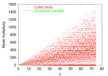
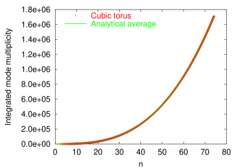
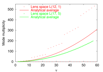
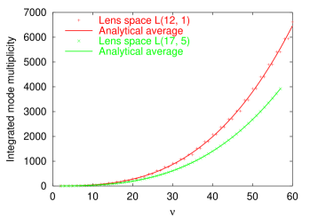
Figure 2: Multiplicity of the mode $k$ as a function of $n$ (cubic torus, top panels) or $\nu$ (lens space $L(p,q)$, bottom panels). For the cubic torus, $n$ is of the form $\sqrt{N}$, where $N$ is an integer, and for lens spaces (and more generally spherical spaces), $\nu$ is an integer. Left panels show the multiplicity of each mode for a given value of either $n$ of $\nu$. We have also given an estimate of the “average” number of modes, given by $2\pi n$ for the torus and $(\nu+1)^{2}/p$ for the lens spaces, respectively. For lens space $L(17,5)$, the mode multiplicity closely follows the analytical estimate, whereas for lens space $L(12,1)$, modes exist only for even values of $\nu$. For the cubic torus, the mode multiplicity is even more irregular, and varies between $0$ and $\sim 20n$. For example, it is always $0$ when $n=\sqrt{8m+7}$. Right panels show the integrated mode multiplicity, that is the number of modes smaller or equal to some value ($2\pi n/L$ and $(\nu+1)\sqrt{K}$, respectively). Here, the analytical estimates ($4\pi n^{3}/3$ and $(\nu+1)(\nu+2)(2\nu+3)/6p$, respectively) provide a much better estimation (see Section 5 of Ref. [14] for a detailed discussion of these properties).

so that the label $s$ can be chosen to be the “unit” integer vector ${\bf\hat{n}}$. The label multiplicity ${\rm mult}(k)\equiv{\rm card}\{s\}$ of a mode $k$ is given in this case by the number of representations of $n^{2}$ by 3 squares, i.e., by ${\rm card}\{{\bf\hat{n}}\}$ (see Fig. 2 below). The corresponding normalized eigenmodes in Cartesian coordinates are thus simply given by

$$\Upsilon^{[{T_{1}}]}_{{k}\,{{\bf\hat{n}}}}({\bf r})=\frac{{\rm e}^{i{\bf k}\cdot{\bf r}}}{(2\pi)^{3/2}},$$ (34)

with ${\bf k}$ given by Eq. (29). Using the decomposition (129) of the exponential and plugging in the closure relation (127), one gets that

$$\xi^{[{T_{1}}]\,{s}}_{{k}\,{\ell}\,{m}}=\xi^{[{T_{1}}]\,{{\bf\hat{n}}}}_{{2\pi n/L}\,{\ell}\,{m}}=i^{\ell}Y_{\ell}^{m}{}^{*}({\bf\hat{n}}),$$ (35)

where ${\bf\hat{n}}$ can also be defined by the two spherical angles $(\theta_{{\bf n}}$, $\varphi_{{\bf n}})$ which are explicitly given by

$$\tan\theta_{\bf n} = \frac{\sqrt{n_{1}^{2}+n_{2}^{2}}}{n_{3}},$$ (36)

$$\tan\varphi_{\bf n} = \frac{n_{2}}{n_{1}}.$$ (37)

This expression could also have been obtained by simply considering the Fourier transform of ${\cal Y}^{[{{\bf R}^{3}}]}_{{k}\,{\ell}\,{m}}$ as given by Eq. (128). One can check that the normalization of the basis $\Upsilon^{[{T_{1}}]}_{{k}\,{{\bf\hat{n}}}}$ [i.e., $\int\Upsilon^{[{T_{1}}]}_{{k}\,{{\bf\hat{n}}}}\Upsilon^{[{T_{1}}]}_{{k^{\prime}}\,{{\bf\hat{n}}^{\prime}}}{}^{*}{\rm d}^{3}{\bf x}=\delta^{{\rm D}}({{\bf k}-{\bf k}^{\prime}})$] implies that the coefficients $\xi^{[{T_{1}}]\,{{\bf\hat{n}}}}_{{k}\,{\ell}\,{m}}$ satisfy the closure relation

$$\sum_{\ell=0}^{\infty}\sum_{m=-\ell}^{\ell}\xi^{[{T_{1}}]\,{{\bf\hat{n}}}}_{{k}\,{\ell}\,{m}}\,\xi^{[{T_{1}}]\,{{\bf\hat{n}}^{\prime}\;*}}_{{k^{\prime}}\,{\ell}\,{m}}=\delta^{{\rm D}}({\cos\theta_{\bf n}-\cos\theta_{{\bf n}^{\prime}}})\delta^{{\rm D}}({\varphi_{\bf n}-\varphi_{{\bf n}^{\prime}}})\delta_{{k}\,{k^{\prime}}}.$$ (38)

The Dirac distribution in the above expression can be shown, by using either Eqs. (126,127) or Eq. (130) alone, to be

$$\delta^{{\rm D}}({\cos\theta_{\bf n}-\cos\theta_{{\bf n}^{\prime}}})\delta^{{\rm D}}({\varphi_{\bf n}-\varphi_{{\bf n}^{\prime}}})=\sum_{\ell=0}^{\infty}\frac{2\ell+1}{4\pi}P_{\ell}({\bf\hat{n}}.{\bf\hat{n}}^{\prime}).$$ (39)

¿From these results, we deduce that the correlation matrix of the $a_{{\ell}\,{m}}$ is given by

$$C_{{\ell}\,{m}}^{{\ell^{\prime}}\,{m^{\prime}}}=\left(\frac{2\pi}{L}\right)^{3}\sum_{n}i^{\ell-\ell^{\prime}}{\cal P}_{\phi}\left(\frac{2\pi n}{L}\right)G_{\ell}\left(\frac{2\pi n}{L}\right)G_{\ell^{\prime}}\left(\frac{2\pi n}{L}\right)\sum_{\bf\hat{n}}Y_{\ell}^{m}{}^{*}({\bf\hat{n}})Y_{\ell^{\prime}}^{m^{\prime}}({\bf\hat{n}}).$$ (40)

Using Eq. (127) and the fact that $\sum_{n,{\bf\hat{n}}}=\sum_{{\bf n}}$, the $C_{\ell}$ coefficients are simply

$$C_{\ell}=\frac{1}{2\pi}\left(\frac{2\pi}{L}\right)^{3}\sum_{{\bf n}}{\cal P}_{\phi}\left(\frac{2\pi n}{L}\right)G_{\ell}^{2}\left(\frac{2\pi n}{L}\right),$$ (41)

which was used in many earlier works [3, 4, 5, 6] on the influence of topology on the CMB.

Note that spherical harmonics satisfy the following symmetry relation

$$Y_{\ell}^{m}(\theta,-\varphi)={\rm e}^{-2im\varphi}Y_{\ell}^{m}(\theta,\varphi).$$ (42)

Due to the symmetry of the torus with respect to the $y=0$ plane, in the sum over ${\bf\hat{n}}$ in Eq. (40) a term $(\theta_{\bf n},\varphi_{\bf n})$ will always be associated to a term $(\theta_{\bf n},-\varphi_{\bf n})$ leading to a term of the form $4\cos\left((m^{\prime}-m)\varphi_{\bf n}\right)Y_{\ell}^{m}{}^{*}(\theta_{\bf n},0)Y_{\ell^{\prime}}^{m^{\prime}}(\theta_{\bf n},0)$, the only exception being the term arising when $n_{2}=0$, which is real. ¿From this result, one easily shows that the correlation matrix satisfies

$$C_{{\ell}\,{m}}^{{\ell^{\prime}}\,{m^{\prime}}}\in{\bf R}.$$ (43)

Along similar lines, the relations

$$Y_{\ell}^{m}(\theta,\pi) = \hbox{e}^{im\varphi}Y_{\ell}^{m}(\theta,0),$$ (44)

$$Y_{\ell}^{m}(\pi-\theta,\varphi) = (-1)^{\ell+m}Y_{\ell}^{m}(\theta,\varphi),$$ (45)

imply

$$C_{{\ell}\,{m}}^{{\ell^{\prime}}\,{m^{\prime}}}=\frac{1}{4}\left[1+(-1)^{m-m^{\prime}}\right]\left[1+(-1)^{\ell-\ell^{\prime}}\right]C_{{\ell}\,{m}}^{{\ell^{\prime}}\,{m^{\prime}}},$$ (46)

so that

$$C_{{\ell}\,{m}}^{{\ell^{\prime}}\,{m^{\prime}}}\neq 0\quad\Rightarrow\quad m-m^{\prime}\equiv 0\>\;{\rm mod}({2})\quad{\rm and}\quad\ell-\ell^{\prime}\equiv 0\>\;{\rm mod}({2}).$$ (47)

Furthermore Eqs.(43,124) imply

$$C_{{\ell}\,{m}}^{{\ell^{\prime}}\,{m^{\prime}}}=C_{{\ell}\,{-m}}^{{\ell^{\prime}}\,{-m^{\prime}}}.$$ (48)

Let us emphasize that these properties of the correlation matrix still hold even if the torus is not cubic. However, a cubic torus is invariant under a $\pi/2$-rotation about the $z$ axis, so if $(n_{1},n_{2},n_{3})$ corresponds to a wavenumber then so does $(n_{2},-n_{1},n_{3})$, and one has

$$C_{{\ell}\,{m}}^{{\ell^{\prime}}\,{m^{\prime}}}\neq 0\quad\Rightarrow\quad m-m^{\prime}\equiv 0\>\;{\rm mod}({4}).$$ (49)

III.2 Spherical spaces

The goal of this section is to recall the basic analytical results concerning the lens and prism spaces (Sec. III.2.2). In these spaces, the eigenmodes and eigenvalues of the Laplacian operator can be determined analytically using toroidal coordinates [36]. CMB computations use spherical coordinates, so we must perform a change of coordinates and a change of basis (detailed in Appendix B). Fortunately, this can also be achieved analytically to compute the coefficients $\xi^{[{\Gamma}]\,{s}}_{{k}\,{\ell}\,{m}}$.

III.2.1 Generalities

In our preceding article [35], we presented in a pedestrian way the complete classification of three-dimensional spherical topologies and we described how to compute their holonomy transformations.

The isometry group of the $3$-sphere is $\rm{SO}({4})$. Every isometry in $\rm{SO}({4})$ can be decomposed as the product of a right-handed and a left-handed Clifford translation, and the factorization is unique up to simultaneous multiplication of both factors by -1. Furthermore, the space ${\bf S}^{3}$ itself enjoys a group structure as the set ${\cal S}^{3}$ of unit length quaternions. Each right-handed (resp. left-handed) Clifford translation corresponds to left (resp. right) quaternion multiplication of ${\cal S}^{3}$, so the group of right-handed (resp. left-handed) Clifford translations is isomorphic to ${\cal S}^{3}$. It follows that $\rm{SO}({4})$ is isomorphic to ${\cal S}^{3}\times{\cal S}^{3}/\{\pm({\bf 1},{\bf 1})\}$ and thus the classification of the subgroups of $\rm{SO}({4})$ can be deduced from the classification of subgroups of ${\cal S}^{3}$. There is a two-to-one homomorphism from ${\cal S}^{3}$ to $\rm{SO}({3})$; the finite subgroups of $\rm{SO}({3})$ are the cyclic, dihedral, tetrahedral, octahedral and icosahedral groups, so the finite subgroups of ${\cal S}^{3}$ are their lifts, namely

• the cyclic groups $Z_{n}$ of order $n$,

• the binary dihedral groups $D_{m}^{*}$ of order $4m$, $m\geq 2$,

• the binary tetrahedral group $T^{*}$ of order 24,

• the binary octahedral group $O^{*}$ of order 48,

• the binary icosahedral group $I^{*}$ of order 120,

where a binary group is the two-fold cover of the corresponding plain group.

¿From this classification, it can be shown that there are three categories of spherical 3-manifolds.

• The single action manifolds are those for which a subgroup $R$ (resp. $L$) of ${\cal S}^{3}$ acts as pure right-handed (resp. pure left-handed) Clifford translations. They are thus the simplest spherical manifolds and can all be written as ${\bf S}^{3}/\Gamma$ with $\Gamma=Z_{n},D_{m}^{*},T^{*},O^{*},I^{*}$.

• The double-action manifolds are those for which subgroups $R$ and $L$ of ${\cal S}^{3}$ act simultaneously as right- and left-handed Clifford translations, and every element of $R$ occurs with every element of $L$. There are obtained for the groups $\Gamma=\Gamma_{1}\times\Gamma_{2}$ with $(\Gamma_{1},\Gamma_{2})=(Z_{m},Z_{n})$, $(D^{*}_{m},Z_{n})$, $(T^{*},Z_{n})$, $(O^{*},Z_{n})$, $(I^{*},Z_{n})$, with ${\rm gcd}(m,n)=1$, ${\rm gcd}(4m,n)=1$, ${\rm gcd}(24,n)=1$, ${\rm gcd}(48,n)=1$, and ${\rm gcd}(120,n)=1$, respectively.

• The linked-action manifolds are similar to the double action manifolds, except that each element of $R$ occurs with only some of the elements of $L$.

The classification of these manifolds is summarized in Fig. 8 of Ref. [35].

III.2.2 Lens and prism spaces

In this article, we focus on prism spaces ${\bf S}^{3}/D_{m}^{*}$ and lens spaces $L(p,q)$ . The latter are defined by identifying the lower surface of a lens-shaped solid to the upper surface with a rotation of angle $2\pi q/p$ for $p$ and $q$ relatively prime integers with $0<q<p$. Furthermore, we may restrict our attention to $0<q\leq p/2$ because for values of $q$ in the range $p/2<q<p$ the twist $2\pi q/p$ is the same as $-2\pi(p-q)/p$, thus $L(p,q)$ is the mirror image of $L(p,p-q)$. Lens spaces can be single action, double action, or linked action; Fig. 9 of Ref. [35] summarizes their classification.

The eigenmodes and eigenvalues of prism and lens spaces can be obtained analytically by working in toroidal coordinates [36]. Starting from Cartesian coordinates, in which the equation for the $3$-sphere is $x^{2}+y^{2}+z^{2}+w^{2}=1$, the toroidal coordinates $(\chi_{\scriptscriptstyle{\rm T}},\theta_{\scriptscriptstyle{\rm T}},\varphi_{\scriptscriptstyle{\rm T}})$ are defined via the equations

$$x = \cos\chi_{\scriptscriptstyle{\rm T}}\,\cos\theta_{\scriptscriptstyle{\rm T}},$$ (50)

$$y = \cos\chi_{\scriptscriptstyle{\rm T}}\,\sin\theta_{\scriptscriptstyle{\rm T}},$$ (51)

$$z = \sin\chi_{\scriptscriptstyle{\rm T}}\,\cos\varphi_{\scriptscriptstyle{\rm T}},$$ (52)

$$w = \sin\chi_{\scriptscriptstyle{\rm T}}\,\sin\varphi_{\scriptscriptstyle{\rm T}},$$ (53)

with

$$0 \leq \chi_{\scriptscriptstyle{\rm T}}\leq\pi/2,$$ (54)

$$0 \leq \theta_{\scriptscriptstyle{\rm T}}\leq 2\pi,$$ (55)

$$0 \leq \varphi_{\scriptscriptstyle{\rm T}}\leq 2\pi.$$ (56)

Ref. [36] gives the eigenmodes of ${\bf S}^{3}$ explicitly as

$${\cal Q}_{{\nu}\,{\ell_{\scriptscriptstyle{\rm T}}}\,{m_{\scriptscriptstyle{\rm T}}}}=B_{{\nu}\,{\ell_{\scriptscriptstyle{\rm T}}}\,{m_{\scriptscriptstyle{\rm T}}}}\cos^{|\ell_{\scriptscriptstyle{\rm T}}|}\chi_{\scriptscriptstyle{\rm T}}\;\sin^{|m_{\scriptscriptstyle{\rm T}}|}\chi_{\scriptscriptstyle{\rm T}}\;P_{d}^{({|m_{\scriptscriptstyle{\rm T}}|}\,,\,{|\ell_{\scriptscriptstyle{\rm T}}|})}(\cos 2\chi_{\scriptscriptstyle{\rm T}})f(|\ell_{\scriptscriptstyle{\rm T}}|\theta_{\scriptscriptstyle{\rm T}})f(|m_{\scriptscriptstyle{\rm T}}|\varphi_{\scriptscriptstyle{\rm T}}),$$ (57)

where $\nu$ is the integer parameterizing $k=(\nu+1)\sqrt{K}$ as in Eqn. (5), $P_{d}^{({|m_{\scriptscriptstyle{\rm T}}|}\,,\,{|\ell_{\scriptscriptstyle{\rm T}}|})}$ is the Jacobi polynomial, and $f$ stands for the cosine (resp. sine) function when $\ell_{\scriptscriptstyle{\rm T}}$ or $m_{\scriptscriptstyle{\rm T}}\geq 0$ (resp. $\ell_{\scriptscriptstyle{\rm T}}$ or $m_{\scriptscriptstyle{\rm T}}<0$). For each value of $\nu$, the indices $\ell_{\scriptscriptstyle{\rm T}}$ and $m_{\scriptscriptstyle{\rm T}}$ range over all integers satisfying

$$|\ell_{\scriptscriptstyle{\rm T}}|+|m_{\scriptscriptstyle{\rm T}}| \leq \nu\qquad{\rm and}$$ (58)

$$|\ell_{\scriptscriptstyle{\rm T}}|+|m_{\scriptscriptstyle{\rm T}}| \equiv \nu\>\;{\rm mod}({2}),$$ (59)

and for convenience we define

$$d=\frac{1}{2}(\nu-|\ell_{\scriptscriptstyle{\rm T}}|-|m_{\scriptscriptstyle{\rm T}}|).$$ (60)

The normalization coefficients $B_{{\nu}\,{\ell_{\scriptscriptstyle{\rm T}}}\,{m_{\scriptscriptstyle{\rm T}}}}$ are given by

$$B_{{\nu}\,{\ell_{\scriptscriptstyle{\rm T}}}\,{m_{\scriptscriptstyle{\rm T}}}}=\frac{\sigma_{\ell_{\scriptscriptstyle{\rm T}}}\sigma_{m_{\scriptscriptstyle{\rm T}}}}{\pi(\nu+1)}\sqrt{\frac{2(\nu+1)\,d!\,(|\ell_{\scriptscriptstyle{\rm T}}|+|m_{\scriptscriptstyle{\rm T}}|+d)!}{(|\ell_{\scriptscriptstyle{\rm T}}|+d)!\,(|m_{\scriptscriptstyle{\rm T}}|+d)!}}$$ (61)

with $\sigma_{i}=1/\sqrt{2}$ if $i=0$ and $\sigma_{i}=1$ otherwise.

Using these definitions, Ref. [36] shows that for lens spaces the explicit set of coefficients $\eta^{[{\Gamma}]\,{\nu}}_{{s}\,{\ell_{\scriptscriptstyle{\rm T}}}\,{m_{\scriptscriptstyle{\rm T}}}}$ such that

$$\Upsilon^{[{\Gamma}]}_{{k}\,{s}}=\sum_{\ell_{\scriptscriptstyle{\rm T}},m_{\scriptscriptstyle{\rm T}}}\eta^{[{\Gamma}]\,{s}}_{{\nu}\,{\ell_{\scriptscriptstyle{\rm T}}}\,{m_{\scriptscriptstyle{\rm T}}}}{\cal Q}_{{\nu}\,{\ell_{\scriptscriptstyle{\rm T}}}\,{m_{\scriptscriptstyle{\rm T}}}}(\chi_{\scriptscriptstyle{\rm T}},\theta_{\scriptscriptstyle{\rm T}},\varphi_{\scriptscriptstyle{\rm T}}),$$ (62)

can be obtained as follows:

Theorem 1: lens spaces

The eigenspace of the Laplacian on the lens space $L(p,q)$ has an orthonormal basis that, when lifted to $Z_{p}$-invariant eigenmodes of the $3$-sphere, comprises those eigenmodes in the left column for which the corresponding condition in the right column is satisfied, subject to the restriction that an eigenmode ${\cal Q}_{{\nu}\,{\ell_{\scriptscriptstyle{\rm T}}}\,{m_{\scriptscriptstyle{\rm T}}}}$ exists if and only if the integers $\nu$, $\ell_{\scriptscriptstyle{\rm T}}$, and $m_{\scriptscriptstyle{\rm T}}$ satisfy $|\ell_{\scriptscriptstyle{\rm T}}|+|m_{\scriptscriptstyle{\rm T}}|\leq\nu$ and $|\ell_{\scriptscriptstyle{\rm T}}|+|m_{\scriptscriptstyle{\rm T}}|\equiv\nu\>\;{\rm mod}({2})$.

basis vectors		condition
${\cal Q}_{{\nu}\,{0}\,{0}}$		always
${\cal Q}_{{\nu}\,{\ell_{\scriptscriptstyle{\rm T}}}\,{0}}$		$\ell_{\scriptscriptstyle{\rm T}}\equiv 0\>\;{\rm mod}({p})$
${\cal Q}_{{\nu}\,{0}\,{m_{\scriptscriptstyle{\rm T}}}}$		$qm_{\scriptscriptstyle{\rm T}}\equiv 0\>\;{\rm mod}({p})$
$({\cal Q}_{{\nu}\,{\ell_{\scriptscriptstyle{\rm T}}}\,{m_{\scriptscriptstyle{\rm T}}}}+{\cal Q}_{{\nu}\,{-\ell_{\scriptscriptstyle{\rm T}}}\,{-m_{\scriptscriptstyle{\rm T}}}})/\sqrt{2},\quad({\cal Q}_{{\nu}\,{-\ell_{\scriptscriptstyle{\rm T}}}\,{m_{\scriptscriptstyle{\rm T}}}}-{\cal Q}_{{\nu}\,{\ell_{\scriptscriptstyle{\rm T}}}\,{-m_{\scriptscriptstyle{\rm T}}}})/\sqrt{2}$		$\ell_{\scriptscriptstyle{\rm T}}\equiv qm_{\scriptscriptstyle{\rm T}}\>\;{\rm mod}({p})$
$({\cal Q}_{{\nu}\,{\ell_{\scriptscriptstyle{\rm T}}}\,{m_{\scriptscriptstyle{\rm T}}}}-{\cal Q}_{{\nu}\,{-\ell_{\scriptscriptstyle{\rm T}}}\,{-m_{\scriptscriptstyle{\rm T}}}})/\sqrt{2},\quad({\cal Q}_{{\nu}\,{-\ell_{\scriptscriptstyle{\rm T}}}\,{m_{\scriptscriptstyle{\rm T}}}}+{\cal Q}_{{\nu}\,{\ell_{\scriptscriptstyle{\rm T}}}\,{-m_{\scriptscriptstyle{\rm T}}}})/\sqrt{2}$		$\ell_{\scriptscriptstyle{\rm T}}\equiv-qm_{\scriptscriptstyle{\rm T}}\>\;{\rm mod}({p})$

An analogous theorem was demonstrated for prism spaces and can be found in Ref. [36].

Unfortunately, for practical purposes the eigenmodes of the lens and prism spaces are needed in spherical coordinates, while they are most easily obtained in toroidal coordinates. As explained in the Introduction, one needs the coefficients $\xi^{[{\Gamma}]\,{s}}_{{k}\,{\ell}\,{m}}$ of the decomposition (4). Since ${\cal Y}^{[{{\bf S}^{3}}]}_{{k}\,{\ell}\,{m}}$ and ${\cal Q}_{{\nu}\,{\ell_{\scriptscriptstyle{\rm T}}}\,{m_{\scriptscriptstyle{\rm T}}}}$ are two orthogonal bases of dimension $(\nu+1)^{2}$, all of whose elements have the same norm, there is an orthogonal transformation taking one to the other

$${\cal Q}_{{\nu}\,{\ell_{\scriptscriptstyle{\rm T}}}\,{m_{\scriptscriptstyle{\rm T}}}}=\sum_{\ell,m}\alpha_{{\nu}\,{\ell}\,{m}\,{\ell_{\scriptscriptstyle{\rm T}}}\,{m_{\scriptscriptstyle{\rm T}}}}{\cal Y}^{[{{\bf S}^{3}}]}_{{k}\,{\ell}\,{m}}.$$ (63)

The “transpose” of this transformation $\alpha$ takes a given eigenmode’s ${\cal Q}$-based coefficients $\eta$ to its ${\cal Y}$-based coefficients $\xi$:

$$\xi^{[{\Gamma}]\,{s}}_{{k}\,{\ell}\,{m}}=\sum_{\ell_{\scriptscriptstyle{\rm T}}=-\nu}^{\nu}\sum_{m_{\scriptscriptstyle{\rm T}}=-\nu}^{\nu}\alpha_{{\nu}\,{\ell}\,{m}\,{\ell_{\scriptscriptstyle{\rm T}}}\,{m_{\scriptscriptstyle{\rm T}}}}\eta^{[{\Gamma}]\,{\nu}}_{{s}\,{\ell_{\scriptscriptstyle{\rm T}}}\,{m_{\scriptscriptstyle{\rm T}}}}.$$ (64)

The orthonormality of the basis $\Upsilon^{[{\Gamma}]}_{{k}\,{s}}$ implies that the coefficients $\xi^{[{\Gamma}]\,{s}}_{{k}\,{\ell}\,{m}}$ satisfy

$$\sum_{\ell=0}^{\nu}\sum_{m=-\ell}^{\ell}\xi^{[{\Gamma}]\,{s}}_{{k}\,{\ell}\,{m}}\xi^{[{\Gamma}]\,{s^{\prime}\;*}}_{{k}\,{\ell}\,{m}}=\delta_{{s}\,{s^{\prime}}}.$$ (65)

This relation is simpler than the closure relation (38) obtained in the flat case because, for a given $k$, the space of modes is finite-dimensional. The computation of the coefficients $\alpha_{{\nu}\,{\ell}\,{m}\,{\ell_{\scriptscriptstyle{\rm T}}}\,{m_{\scriptscriptstyle{\rm T}}}}$ appears in Appendix B. Because both the ${\cal Q}$ basis and the ${\cal Y}$ basis are orthonormal, the transformation $\alpha$ is orthogonal:

$$\sum_{\ell=0}^{\nu}\sum_{m=-\ell}^{\ell}\alpha_{{\nu}\,{\ell}\,{m}\,{\ell_{\scriptscriptstyle{\rm T}}}\,{m_{\scriptscriptstyle{\rm T}}}}\alpha_{{\nu}\,{\ell}\,{m}\,{\ell_{\scriptscriptstyle{\rm T}}^{\prime}}\,{m_{\scriptscriptstyle{\rm T}}^{\prime}}}^{*}=\delta_{{\ell_{\scriptscriptstyle{\rm T}}}\,{\ell_{\scriptscriptstyle{\rm T}}^{\prime}}}\delta_{{m_{\scriptscriptstyle{\rm T}}}\,{m_{\scriptscriptstyle{\rm T}}^{\prime}}}\varepsilon_{\nu}(\ell_{\scriptscriptstyle{\rm T}},m_{\scriptscriptstyle{\rm T}})\varepsilon_{\nu}(\ell_{\scriptscriptstyle{\rm T}}^{\prime},m_{\scriptscriptstyle{\rm T}}^{\prime})$$ (66)

where $\varepsilon_{\nu}(\ell_{\scriptscriptstyle{\rm T}},m_{\scriptscriptstyle{\rm T}})=1$ if the conditions (58,59) are satisfied and 0 otherwise.

With these coefficients, the CMB computation goes as in the flat case, except for the fact that some integrals have to be replaced by discrete sums. One easily gets that

$$\frac{\delta T}{T}(\theta,\varphi)=\frac{(2\pi)^{3}}{V}\sum_{\nu=2}^{\infty}\sum_{s}\sum_{\ell,m}\xi^{[{\Gamma}]\,{s}}_{{k}\,{\ell}\,{m}}O_{k}^{[{\bf S}^{3}]}\left({\cal Y}^{[{{\bf S}^{3}}]}_{{k}\,{\ell}\,{m}}\right)\sqrt{{\cal P}_{\phi}(k)}\,\hat{e}_{\bf k},$$ (67)

so that

$$a_{{\ell}\,{m}}=\frac{(2\pi)^{3}}{V}\sum_{\nu=2}^{\infty}\sqrt{{\cal P}_{\phi}(k)}\,O_{k}^{[{\bf S}^{3}]}\left(R^{[{{\bf S}^{3}}]}_{{k}\,{\ell}}\right)\sum_{s}\xi^{[{\Gamma}]\,{s}}_{{k}\,{\ell}\,{m}}\hat{e}_{\bf k},$$ (68)

and

$$C_{{\ell}\,{m}}^{{\ell^{\prime}}\,{m^{\prime}}}=\frac{(2\pi)^{3}}{V}\sum_{\nu=2}^{\infty}{\cal P}_{\phi}(k)G_{\ell}(k)G_{\ell^{\prime}}(k)\sum_{s}\xi^{[{\Gamma}]\,{s}}_{{k}\,{\ell}\,{m}}\xi^{[{\Gamma}]\,{s\;*}}_{{k}\,{\ell^{\prime}}\,{m^{\prime}}},$$ (69)

as first obtained in Ref. [14]. Note also that, following Refs. [53, 54], a scale invariant spectrum will in that case be defined as

$${\cal P}_{\phi}(k)\propto\frac{1}{k(k^{2}-K)}.$$ (70)

To finish, let us discuss the properties of the random variable $\hat{e}_{\bf k}$. Since the eigenmodes in toroidal coordinates, ${\cal Q}_{{\nu}\,{\ell_{\scriptscriptstyle{\rm T}}}\,{m_{\scriptscriptstyle{\rm T}}}}$, and the coefficients $\eta^{[{\Gamma}]\,{s}}_{{\nu}\,{\ell_{\scriptscriptstyle{\rm T}}}\,{m_{\scriptscriptstyle{\rm T}}}}$ are real valued, it follows from Eq. (C2) that

$$\alpha_{{\nu}\,{\ell}\,{m}\,{\ell_{\scriptscriptstyle{\rm T}}}\,{m_{\scriptscriptstyle{\rm T}}}}^{*}=(-1)^{m}\alpha_{{\nu}\,{\ell}\,{-m}\,{\ell_{\scriptscriptstyle{\rm T}}}\,{m_{\scriptscriptstyle{\rm T}}}}.$$ (71)

It follows that

$${\xi^{[{\Gamma}]\,{s}}_{{k}\,{\ell}\,{m}}}^{*}=(-1)^{m}\xi^{[{\Gamma}]\,{s}}_{{k}\,{\ell}\,{-m}},$$ (72)

whatever $s$ and thus that the eigenmodes $\Upsilon^{[{\Gamma}]}_{{k}\,{s}}$ are real-valued. This implies that $\hat{e}_{\bf k}$ is a real random variable, contrary to the preceding example of the torus.

IV Numerical computations

IV.1 Implementation

The correlation matrix for $\ell\leq\ell_{\rm max}$ has $\ell_{\rm max}^{4}$ coefficients. However, the parity and symmetry relations

$$C_{{\ell}\,{m}}^{{\ell^{\prime}}\,{m^{\prime}}} = (-1)^{m-m^{\prime}}C_{{\ell}\,{-m}}^{{\ell^{\prime}}\,{-m^{\prime}}}{}^{*}$$ (73)

$$C_{{\ell}\,{m}}^{{\ell^{\prime}}\,{m^{\prime}}} = C_{{\ell^{\prime}}\,{m^{\prime}}}^{{\ell}\,{m}}{}^{*}$$ (74)

reduce the problem to computing only a quarter of them. Then, for a given topology, symmetries can further reduce the number of coefficients to compute. For example, with a cubic torus, Eqs. (47,49) insure that only one coefficient out of eight is nonzero, and the symmetries (48) also give the coefficients when one changes the sign of both $m$ and $m^{\prime}$. This leaves only $\ell_{\rm max}^{4}/64$ coefficients to compute. For example, a COBE scale map ($\ell_{\rm max}\sim 30$) requires $12500$ coefficients, while a Planck scale map ($\ell_{\rm max}\sim 1500$) requires $\sim 8\times 10^{10}$ coefficients.

Each coefficients is computed using Eq. (40), which involves a sum over all the wavemodes ${\bf k}$. For a given resolution $\ell_{\rm max}$ the modulus of the largest wavemode is given by $k_{\rm max}\sim 3\ell_{\rm max}/\eta_{0}$. Moreover, the density of wavemodes is proportional to the size of the torus, so that we have $O(\ell_{\rm max}^{3}L^{3})$ modes. Therefore, the computational time and the memory requirement scale as $\ell_{\rm max}^{7}L^{3}$ and $\ell_{\rm max}^{3}L^{3}$, respectively. This is obviously a serious limitation of our algorithm. For example, computing the correlation matrix for a COBE scale map on a relatively small torus ($L=2R_{H}$, where $R_{H}$ is the Hubble radius) takes around $10$ hours on a $900\,{\mbox{MHz}}$ CPU and allocates $60$ Megabytes of memory.

When the topology is simply connected, it is a well-known fact that the $C_{\ell}$ are in general a smooth function of the multipole $\ell$. This reduces the computational time because for $\ell_{\rm max}=1500$ one needs to compute only $\sim 50$ coefficients. For the topologies we have studied, we did not find any evidence for a smooth structure of the correlation matrix, at least at the relatively large scales we considered. At which scale one can reliably approximate the correlation matrix by its isotropic diagonal part (the $C_{\ell}$) remains an open question.

Also, if one wants to simulate CMB maps from the correlation matrix, one needs to diagonalize it. This procedure can also take a lot of time because it is an $\ell_{\rm max}^{6}$ process. For the case of the torus, however, this problem is not serious as the symmetries of the torus insure that the matrix is block diagonal, with eight blocks if the torus is cubic or four blocks otherwise.

Strictly speaking, one does not need the correlation matrix to compute maps. One can do it directly by using Eq. (18). This amounts to performing a realization of the three-dimensional random field describing the cosmological perturbations, and projecting it onto the sphere. In this case, one has only $\ell_{\rm max}$ coefficients to compute (the $a_{{\ell}\,{m}}$) instead of the correlation matrix, so that the memory requirements are roughly the same (one only needs to store the value of the random field for each mode), but the computational time scales as $\ell_{\rm max}^{5}L^{3}$. In this case, computing maps for a cubic torus of size $L=2R_{H}$ till $\ell_{\rm max}=120$ takes $3$ hours on a $1.7\,{\mbox{GHz}}$ CPU and allocates 300 Megabytes of memory.

In the case of spherical spaces, the coefficients $\xi^{[{\Gamma}]\,{s}}_{{k}\,{\ell}\,{m}}$ must also be computed numerically. This involves determining both the coefficients $\eta^{[{\Gamma}]\,{\nu}}_{{s}\,{\ell_{\scriptscriptstyle{\rm T}}}\,{m_{\scriptscriptstyle{\rm T}}}}$ and $\alpha_{{\nu}\,{\ell}\,{m}\,{\ell_{\scriptscriptstyle{\rm T}}}\,{m_{\scriptscriptstyle{\rm T}}}}$. This computation can be reduced by taking into account their symmetries, as described in Appendix B, which imply that $\nu-|m|+|\ell_{\scriptscriptstyle{\rm T}}|$ is odd, $|m|=|m_{\scriptscriptstyle{\rm T}}|$, $|\ell_{\scriptscriptstyle{\rm T}}|+|m_{\scriptscriptstyle{\rm T}}|\leq\nu$, and $|\ell_{\scriptscriptstyle{\rm T}}|+|m_{\scriptscriptstyle{\rm T}}|\equiv\nu\>\;{\rm mod}({2})$. The computation can be performed analytically with the use of symbolic computation software such as Mathematica. In the case of the lens space $L(17,5)$, the computation up to $\nu=43$ and $\nu=55$ takes $3$ and $12$ hours respectively on a $1\,{\mbox{Ghz}}$ CPU with a negligible amount of memory.

IV.2 Expected results

The three main effects that are expected on a CMB map computed in a multi-connected topology are (i) the appearance of $\ell$–$\ell^{\prime}$ and $m$–$m^{\prime}$ correlations reflecting the breakdown of global isotropy, (ii) the existence of a cutoff in the CMB angular power spectrum on large angular scales (low $\ell$), and (iii) the existence of pattern correlations such as pairs of circles where the temperature fluctuations are strongly correlated as they represent the intersection of the last scattering surface with itself and therefore show the temperature of the same emission region from different directions. Note that the effects (ii) and (iii) will show up only if the topological scale is smaller than the radius of the last scattering surface while the effect (i) may be present even if the topological scale is a bit larger than the diameter of the last scattering surface.

So far, the main constraints that have been given on multi-connected topologies come from the absence of a cutoff at large angular scales in the COBE spectrum. This gives strong constraints on the minimal size of the topology as the cutoff is given by the angular size of the torus projected on the last scattering surface. However, as previously discussed, this cutoff in the “true” temperature fluctuations can be compensated, at least partially, by an integrated Sachs-Wolfe effect which arises, for example, when the cosmological constant is large.

The third, and up-to-now never computed, effect of a multi-connected topology is the appearance of pairs of circles which are correlated in temperature. This correlation, however, is not perfect. It would be perfect if the temperature fluctuation were a pure scalar function on the last scattering surface $2$-sphere around us which would be the case only if (i) the temperature anisotropies were given only by the Sachs-Wolfe effect [first term of Eq. (20)] and (ii) the last scattering surface were infinitely thin.

It is well-known that the temperature fluctuations observed in a given direction are in fact a combination of several effects: first, one has the intrinsic temperature fluctuations of the emitting region, which is eventually affected by a gravitational redshift. These two contributions form the so-called Sachs-Wolfe effect [first term in the righthand side of Eq. (20)]. Second, if the emission region is not at rest with respect to the observer, one will observe some apparent temperature fluctuations which in fact result from a Doppler shift [second term in the righthand side of Eq. (20)]. Third, several events can alter the photons energy and trajectory while travelling toward us. In particular, they can be slightly disturbed from their trajectory (lensing) and, more importantly, they can exchange energy when they cross time-varying potential wells. This last effect is usually referred to as the integrated Sachs-Wolfe effect [third term in the righthand side of Eq. (20), see Fig. 9 below]. Obviously, the Sachs-Wolfe effect is a scalar quantity that depends only on the emission region. Therefore, it should be the same whatever the direction of observation. By contrast, the Doppler effect will explicitly depend on the direction of observation. If one observes two directions which correspond to the same point of the last scattering surface and which form a small angle, then one expects that the Doppler contribution will be almost the same. If the matching points are $90$ degrees from each other, then one expects on average no correlation at all, whereas the Doppler effect between two antipodal points will become anti-correlated. Finally, since photons originating from the same emission region but observed from different directions will travel through different regions of space, they will undergo different integrated Sachs-Wolfe effects, so that no significant correlations are expected from this effect, which is therefore considered a noise term for our purposes.

Actually, one aim of this work is precisely to compute the typical amount of correlation one can expect on pairs of circles. Note that this correlation is likely to depend on scale: on large scales, one should be annoyed by the late integrated Sachs-Wolfe effect; between the Sachs-Wolfe plateau and the first Doppler peak (and, at a lesser extent, at every dip between two Doppler peaks), the Doppler effect dominates; at the first peak, there is usually (especially when the matter content is low) a significant contribution of the early integrated Sachs-Wolfe effect (see Fig. 9); at very small scales, one feels the finite width of the last scattering surface (see below), etc. Also, as explained above, the relative position of the circles will play a role because of the Doppler contribution. It is therefore interesting to look at the best way to find matching circles on a realistic CMB map. We leave this important point to future work [51].

The second (and probably less important) effect that reduces the correlation between the circles is the finite width of the last scattering surface. As far as we know, this effect has not yet been carefully analyzed. It plays a role when one looks at fluctuations on scales smaller than the projected width of the last scattering surface. In this case when looking in a given direction, one picks up fluctuations which are situated “on one side” of the last scattering surface, but for pairs of circles, one sees opposite sides of the last scattering surface. On larger scales, the effect is negligible as one averages temperature fluctuations on regions much larger than the thickness of the last scattering surface.

V Results

We now outline some of the results we have already obtained from our simulations. The main aim of this Section is to provide a series of tests to check our simulations. A more detailed analysis of the structure of the correlation matrix $C_{{\ell}\,{m}}^{{\ell^{\prime}}\,{m^{\prime}}}$ as well as a search for accurate tests to detect the topology are left for future work [51].

V.1 Flat case: cubic torus

In all the simulations we performed, we have considered a flat $\Lambda$CDM model with $\Omega_{\Lambda}=0.7$, a Hubble parameter of $H_{0}\equiv 100h\,{\mbox{km}}\,{\mbox{s}^{-1}}\,{\mbox{Mpc}^{-1}}$ with $h=0.62$, a baryon density $\omega_{\rm b}\equiv\Omega_{\rm b}h^{2}=0.019$ and a spectral index $n_{\rm S}=1$. With this choice of cosmological parameters, the Hubble radius is $R_{H}\sim 4.8\,{\mbox{Gpc}}$, the “horizon” radius (under the hypothesis of a radiation dominated universe at early times) is $R_{h}\sim 15.6\,{\mbox{Gpc}}$, and the radius of the last scattering surface is $R_{\scriptscriptstyle\rm LSS}\sim 15.3\,{\mbox{Gpc}}$. The volume of the observable universe is therefore $V_{\rm obs}\sim 15\times 10^{3}\,{\mbox{Gpc}^{3}}$.

Let us first compare the $C_{\ell}$ in the simply connected topology to the $C_{\ell}$ in a torus (Fig. 3). As expected, we see a cutoff at some angular size which corresponds to the angular size of the torus on the last scattering surface. This corresponds to the multipole

$$\ell_{c}\sim\frac{2\pi R_{\scriptscriptstyle\rm LSS}}{L},$$ (75)

where $L$ is the length of the cubic torus’ fundamental domain [49, 50]. Note that even when the torus is larger than the size of the observable universe, the spectrum exhibits a loss of power on large scales. This is because the Harrison-Zel’dovich spectrum exhibits a significant amount of power at large scales (by definition, it is scale invariant), and in practice, the modes that contribute to the quadrupole of the CMB anisotropies can be as large as ten times the size of the observable universe (the exact number depends mostly on the spectral index and on the amplitude of the integrated Sachs-Wolfe term). Therefore, this leaves hope to detect the topology “beyond the horizon” where the circles method would fail.

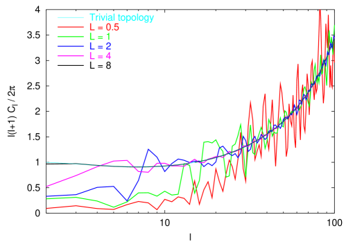
Figure 3: CMB anisotropies in the simply connected (i.e., usual) topology and in toroidal universes based on cubic fundamental domains of various sizes, expressed here in units of the Hubble radius. With our choice of cosmological parameters, the situation $L=8$ corresponds to a torus larger than the observable universe, which shows a small depletion of power on large scales. For smaller tori, the cutoff is much sharper.

It is not easy to predict the amplitude of the power at scales larger than the cutoff because it depends mostly on the amplitude of the integrated Sachs-Wolfe effect, which is difficult to estimate even when the topology is multiconnected. Another consequence of a multiconnected topology are oscillations in the spectrum. These come both from the fact that there is a sharp cutoff in the spectrum (which causes oscillations in Fourier/Legendre space) and that the spectrum is “spiky” on large scales. Should we consider a simply connected universe with a cutoff at some scales, then the corresponding $C_{\ell}$ would be less irregular. Finally, note that on small angular scales, the spectrum tends to behave as in the simply connected case, but computing this scale remains an open problem at the moment.

So far, we have considered only the $C_{\ell}$, which represent only some average of the diagonal part of the correlation matrix. The true diagonal part of the correlation matrix is given by the $C_{{\ell}\,{m}}^{{\ell}\,{m}}$ which represent the variance of the $a_{{\ell}\,{m}}$. An example of their behavior is shown in Fig. 4 for the same topologies as in Fig. 3. Several features appear on this figure. First and most importantly, the dispersion in the variance of the $a_{{\ell}\,{m}}$ at fixed $\ell$ is very large. It appears that it is maximal at the cutoff scale $\ell_{c}$, where the dispersion in the variance of the $a_{{\ell}\,{m}}$ can be as large as two orders of magnitude. This dispersion slowly decays at larger multipoles, where one “tends” (in the sense of observable quantities) towards the simply connected case, and surprisingly also decays at scales larger than the cutoff. With the hypothesis of a multi-connected universe, this dispersion would be (incorrectly) interpreted as non Gaussianity. Since at present no non Gaussianity or anisotropy was observed in the data, this allows new constraints of the size of the fundamental domain.

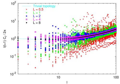
Figure 4: Variance of the $a_{{\ell}\,{m}}$ for fixed values of $\ell$. The average of these values give the $C_{\ell}$ coefficients shown in Fig. 3. We insist that this does not correspond to a realization of the random variables describing CMB anisotropies, but to the variance of the $a_{{\ell}\,{m}}$. These coefficients are far from sufficient to build maps of CMB anisotropies as they do not include the correlations between different $a_{{\ell}\,{m}}$.

We did not find any convenient way to represent the off-diagonal terms of the correlation matrix. We therefore switch to showing and analyzing some realizations corresponding to the numerically computed correlation matrix. In what follows, we have fixed the size of the torus to $L=2R_{H}$. We therefore have $N\sim 16$ copies of the torus in the observable universe, and from Eq. (75) this corresponds to $\ell_{c}\sim 9$, as can be checked in Fig. 3. Although such a model is now excluded by the data [3, 4, 5, 6], we analyze it in detail mostly for pedagogical purposes (and also because the computing time scales as $L^{3}$). In the case where the torus, or more generally the fundamental domain, is smaller than the last scattering surface, one expects to see pairs of circles where the temperature is correlated  [7]. Seeing these circles at their expected position is therefore the most crucial test of the procedure outlined in Secs. II,III,IV. As already announced, the aim here is not to derive a detailed procedure to detect these circles, but to check our algorithm and to explore some of the properties of these matching circles. Here, we have $2R_{\scriptscriptstyle\rm LSS}/L=3.17\sim\sqrt{10}$. One therefore expects to have $61$ pairs of circles and $12$ pairs of points having correlated temperature. In order to see the circles, it is convenient to show the last scattering surface as a sphere seen from the outside and to look at its intersection with itself after a translation of the form $L\cdot(n_{1},n_{2},n_{3})$, as shown in Figs. 5–8.

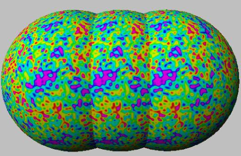
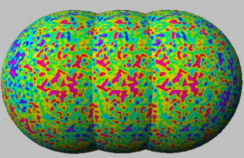
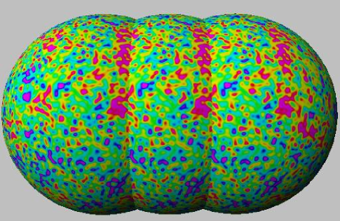
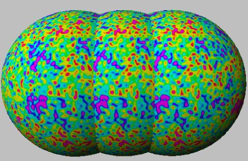
Figure 5: Four realizations of CMB maps of the whole temperature anisotropies for a cubic torus. The resolution of each map is $\ell_{\rm max}=120$ . The last scattering surface is seen from the outside as well as two of its closest topological images after translation of $L$ and $-L$ along one axis of the torus. One can check by eye that the temperature fluctuations are well (but not perfectly) correlated along matching circles (i.e., along the intersection between the last scattering surface and its neighbors) located at latitudes $\theta=\pm 19^{\circ}$. Note that as expected, there are very few fluctuations on scales larger than the size of the torus (which is given here by the distance between the circles).

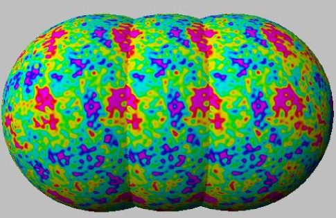
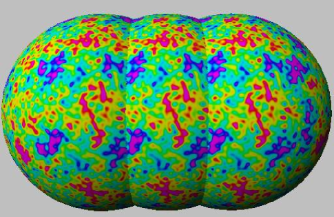
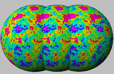
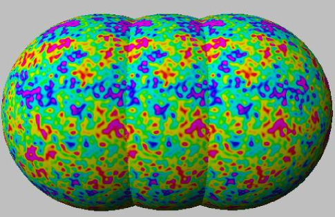
Figure 6: Same as in Fig. 5, but with the Sachs-Wolfe contribution only. These maps have comparatively less small scale power than the previous one as $\ell=120$ is close to the first dip in the Sachs-Wolfe spectrum, so that one sees the large scales (up to the torus angular size) better. Note that the matching between circles is almost perfect here.

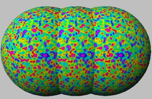
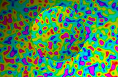
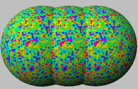
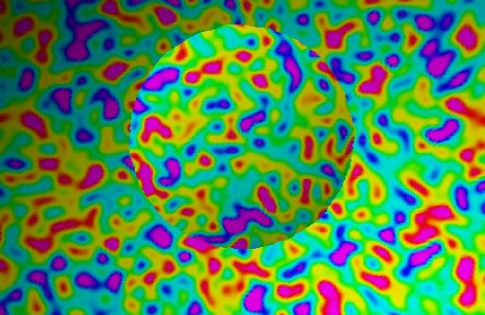
Figure 7: Same as in Fig. 5, but for the Doppler component only. Left panels show as previously the last scattering surface and two of its images from the outside, with large circles, which are therefore well correlated (but not as well as for the Sachs-Wolfe or total contributions, however). On the right panel, we show smaller matching circles ($\theta=\pm 71^{\circ}$), which are more conveniently shown from the inside of the last scattering surface. Here, the anticorrelation between circles is obvious.

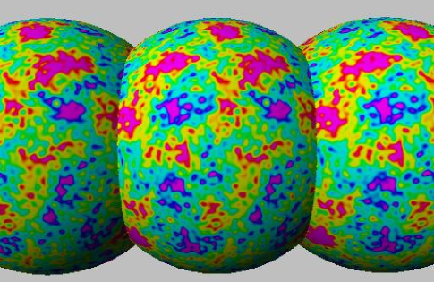
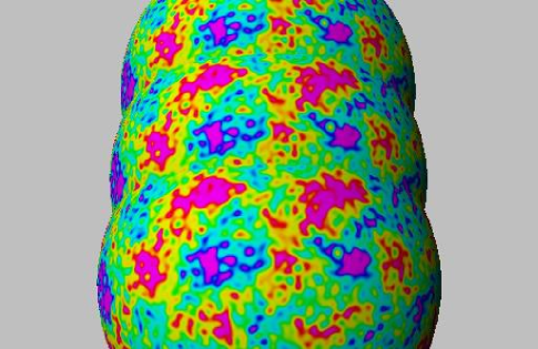
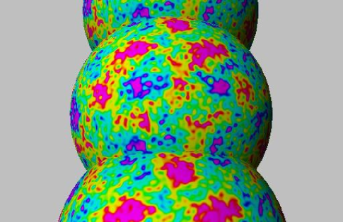
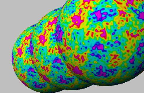
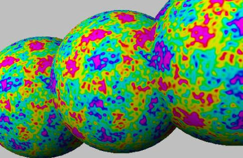
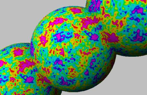
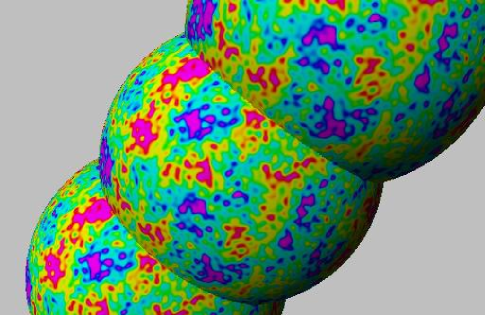
Figure 8: Eight pairs of matching circles among the $61$ existing pairs for a single realization of the density fields. For clarity, the orientation of the last scattering surface is the same in all panels.

In the last Section, we pointed out that the correlation would depend on the amount of Sachs-Wolfe, Doppler and integrated Sachs-Wolfe effects. The decomposition of the temperature anisotropies both in the simply connected topology and in the toroidal cases are shown in Fig. 9. Note that we show only the relative amplitude of these effects and not their cross correlation.

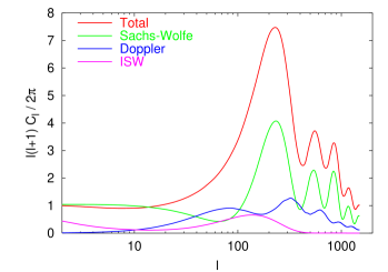
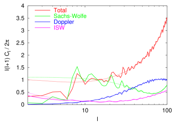
Figure 9: Decomposition of CMB anisotropies into the Sachs-Wolfe, Doppler and ISW contributions. When the topology is simply connected [left panel], the Sachs-Wolfe contribution is dominant at the peaks and usually on the largest scales. The Doppler term is dominant only before the first peak, and has a significant contribution between peaks. The ISW term appears mostly at the first peak (this is referred to as the early ISW effect) when the radiation-to-matter transition occurs late (typically at low $h$), and at large scales (late ISW effect) when the universe is not matter dominated at $z=0$. For standard values of the cosmological parameters, it is not dominant. The right panel shows the initial portion of the spectrum ($\ell\leq 100$) for a model with the same cosmological parameters but with a toroidal topology. The Sachs-Wolfe contribution shows a sharp cutoff at the expected scale. Note that neither the Doppler nor ISW contributions show a similar cutoff. This is due to two different projection effects: for the Doppler term, this comes from the fact that it is always negligible on large scales in $k$ space (it scales as $k^{2}$), and when one goes to $\ell$ space, the convolution (20) always transfers some power from the small scales (where there is power in $k$ space) to large scales; for the ISW, the presence of power comes from the fact that it is generating long after the last scattering epoch, so that it appears on large scales simply because it describes phenomena that occur near us. However, since the Sachs-Wolfe contribution is usually largest on large scales, the final spectrum still exhibits a sharp cutoff.

We now turn to the correlation between pairs of circles, as introduced in  [7].

If the topology is not known in advance, the relative position between matching circles can be arbitrary, so that in general the search for circles is a six parameter problem: two parameters for the center of the first circle, two more for the center of the second circle, one for their common radius, and one for their relative phase (i.e. the twist with which they are identified). In the case of a torus, the circles sit directly opposite each other on the sky (eliminating two parameters) and there is no twist (eliminating another parameter), so the problem reduces to a three parameters search. We are not going to perform such a study, but rather focus on some features of matching circles in a toroidal universe.

A simple estimator for the correlation between pairs of circles that are horizontal with respect to the coordinate system is obviously

$$C(\theta_{1},\theta_{2})\equiv\frac{1}{2\pi}\int\frac{2\Theta(\theta_{1},\varphi)\Theta(\theta_{2},\varphi)}{\Theta^{2}(\theta_{1},\varphi)+\Theta^{2}(\theta_{2},\varphi)}{\rm d}\varphi,$$ (76)

where we have set $\Theta\equiv\delta T/T$. If the temperature fluctuations on a pair of circles are completely uncorrelated, then on average $C=0$. If they are completely correlated, then $C=1$, and if they are anti correlated, then $C=-1$. Each $a_{{\ell}\,{m}}$ can be seen either as the theoretical expectation for a given model, or an observed quantity that can be measured from the CMB sky. In the first case, it represents a feature that one can expect from a given model, and in the second case it represents an estimator of some features predicted by the topology. Here, we shall concentrate on the observed $C(\theta_{1},\theta_{2})$ that we compute from simulated maps, first to check the validity of our procedure to compute the correlation matrix $C_{{\ell}\,{m}}^{{\ell^{\prime}}\,{m^{\prime}}}$, and second to convince us that it is possible to see the presence of matching circles using simple techniques (although we do not pretend that this method is optimal).

In principle, two matching circles have the same angular diameter, so that only the case $\theta_{2}=-\theta_{1}$ is relevant, but we have chosen to leave $\theta_{2}$ as a free parameter to see to what extent uncorrelated circles might happen to seem correlated by chance.

We first show in Fig. 10 a few examples of the observed function $C(\theta_{1},\theta_{2})$ for a simply connected universe. As expected, the correlation is quite large when $\theta_{1}\sim\theta_{2}$ because the circles are near each other and the real space correlation function $C(\theta)$ (the Legendre transform of the $C_{\ell}$) is not 0 when $\theta\to 0$. With our normalization of $C(\theta_{1},\theta_{2})$, one has

$$\lim_{\theta_{2}\to\theta_{1}}C(\theta_{1},\theta_{2})=1,$$ (77)

which will of course remain valid when the topology is multi-connected. When the separation between $\theta_{1}$ and $\theta_{2}$ is large, one can neglect the correlation between the two circles, and the main contribution to $C$ comes from statistical fluctuations: it is always possible that two circles exhibit similar temperature patterns by chance. The variance of these statistical fluctuations is probably given by the number of independent pixels on the map and therefore by a combination of the scale at which the power spectrum is large and of the resolution of the map (here, $\ell_{\rm max}=30$). In any case, the amplitude of the largest statistical fluctuations of $C(\theta_{1},\theta_{2})$ gives an idea of the amplitude of the signal needed to detect a multiconnected topology. For the maps we have generated, the correlation reaches $30\%$ for a few pairs of falsely matched circles.

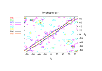
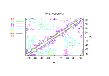
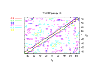
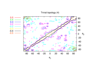
Figure 10: Contour plots of the function $C(\theta_{1},\theta_{2})$ for four realizations of the temperature anisotropies in a universe with a simply connected topology. When $|\theta_{1}-\theta_{2}|$ is small, the correlation between circles exists. When $|\theta_{1}-\theta_{2}|$ is larger, the apparent correlation between circles comes from statistical fluctuations, which would be reduced for higher resolution maps.

Figs. 11, 12, 13 and 14 show contour plots for several realizations of the correlation matrix in a torus universe. The torus aligns naturally with the coordinate system, so one expects correlated pairs of circles at

$$\theta_{1}=-\theta_{2}=\pm\arcsin\left(\frac{nL}{2R_{\scriptscriptstyle\rm LSS}}\right),$$ (78)

for each positive integer $n$ such that the arcsine exists. For our choice of cosmological parameters we have $R_{\scriptscriptstyle\rm LSS}=3.17$ and $L=2$ (in units of the Hubble radius), giving

$$\theta_{1}=-\theta_{2}=\pm 18^{\circ},\pm 39^{\circ},\pm 71^{\circ}.$$ (79)

For these values of $\theta_{1}$ and $\theta_{2}$, one expects a perfect correlation for the Sachs-Wolfe contribution:

$$C_{\rm SW}=1.$$ (80)

This formula holds both when one considers $C_{\rm SW}$ as an ensemble average and when one considers a given realization of the density field since in both cases it follows from the fact that one sees the same region from different directions. These correlations appear clearly in Fig. 11 which considers only the Sachs-Wolfe contribution. In this case one would have even expected perfect correlations for the values of $\theta_{1}$ and $\theta_{2}$ given in (79). This is not what we have, but the reason for this is easy to understand: imposing $\Theta(\theta_{1},\varphi)=\Theta(-\theta_{1},\varphi)$ in real space induces in Legendre space correlations at arbitrary large multipoles $\ell$. Here, for computational reasons, we were forced to truncate the correlation matrix at a rather low value of $\ell$, so the matching is significant but not perfect. It would presumably increase in higher resolution maps.

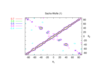
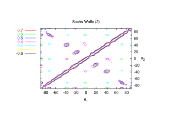
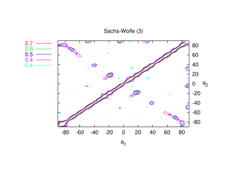
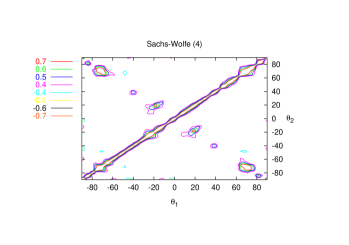
Figure 11: Contour plots of the function $C(\theta_{1},\theta_{2})$ for four realizations of the Sachs-Wolfe part of the temperature anisotropies in a toroidal universe. No large correlations are found except when $|\theta_{1}-\theta_{2}|$ is small and for the three pairs of matching circles.

If one considers the Doppler contribution to the CMB anisotropies, the situation is somewhat different. As announced above, the correlation between two circles depends on their relative angle. More precisely, it is given by

$$C_{\rm Dop}=\left<\frac{2\;({\bf\hat{n}}_{1}\cdot{\bf\hat{n}})\;({\bf\hat{n}}_{2}\cdot{\bf\hat{n}})}{({\bf\hat{n}}_{1}\cdot{\bf\hat{n}})^{2}+({\bf\hat{n}}_{2}\cdot{\bf\hat{n}})^{2}}\right>_{\bf\hat{n}},$$ (81)

where ${\bf\hat{n}}_{1}$ and ${\bf\hat{n}}_{2}$ are two constant unit vectors spanning an angle $|\theta_{1}-\theta_{2}|$, and where the brackets denote an average over all the directions of the unit vector ${\bf\hat{n}}$. After some manipulations, one obtains

$$C_{\rm Dop}=\tan\left(\frac{\pi}{4}-\frac{|\theta_{1}-\theta_{2}|}{2}\right).$$ (82)

Again, for the same reason as for the Sachs-Wolfe contribution, this formula holds both if one considers $C_{\rm Dop}$ as an ensemble average or if we consider a given realization of the density field. One recovers as expected that the correlation is $1$, $0$, $-1$ for $|\theta_{1}-\theta_{2}|=0^{\circ}$, $90^{\circ}$, $180^{\circ}$, respectively. For the values of the angle given in Eq. (79), one obtains $C=0.51$, $0.07$, $-0.49$, respectively. These are the results that we obtain qualitatively in Fig. 12, where no correlation at all is seen for the circles at $\pm 39^{\circ}$, and positive (resp. negative) correlation is seen for the circles at $\pm 71^{\circ}$ (resp. $\pm 18^{\circ}$).

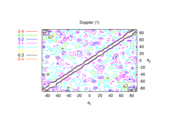
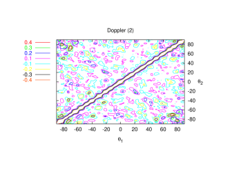
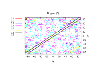
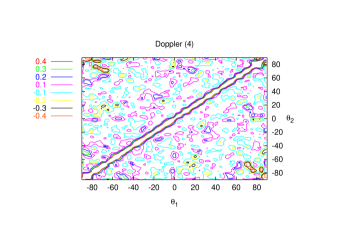
Figure 12: Contour plots of the function $C(\theta_{1},\theta_{2})$ for four realizations of the Doppler part of the temperature anisotropies in a toroidal universe. Some correlation or anti correlation is found for two of the circles, but the signal is not very large compared to the statistical fluctuations. Note that the correlation would have been slightly larger if we would have simulated these maps from a higher resolution correlation matrix.

Finally, the correlations due to the integrated Sachs-Wolfe effect are shown in Fig. 13. As expected, no particular correlation is seen for the values of $\theta_{1}$ and $\theta_{2}$ of Eq. (79). The contour plots are however quite different from those of the Sachs-Wolfe and Doppler contributions. The reason is twofold. First, most of the power lies at the smallest multipoles. This translates into the fact that the contours are broad in the sense that they do not vary a lot on small intervals of $\theta_{1}$ and $\theta_{2}$. Second, the fact that most of the power is at large scales implies that a very small number of modes contributes to it (since we see a finite region of the universe), so there is a large cosmic variance that makes the statistical uncertainty very large (thus serendipitously similar temperature patterns on two unrelated circles are easily achieved here).

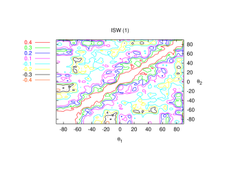
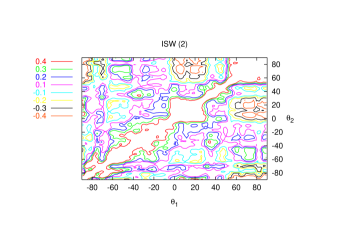
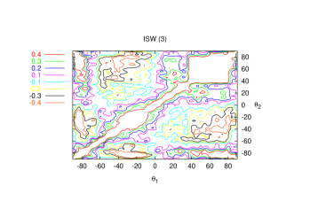
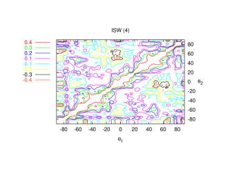
Figure 13: Contour plots of the function $C(\theta_{1},\theta_{2})$ for four realizations of the integrated Sachs-Wolfe part of the temperature anisotropies in a toroidal universe. No significant correlation is seen on the matching circles, whereas large values are found for $|C(\theta_{1},\theta_{2})|$ extending across broad regions as a consequence of the fact that the integrated Sachs-Wolfe effect appears on large angular scales.

Combining all the contributions to the CMB anisotropies allows one to simulate realizations of the exact $C(\theta_{1},\theta_{2})$ as shown in Fig. 14. Since the Sachs-Wolfe contribution is dominant, the spikes are still clearly visible at their expected positions, but appear less prominent than in Fig. 11. As expected, it seems that the circles at $\theta_{1,2}=\pm 39^{\circ}$ are slightly less correlated than the other two pairs because their Doppler contribution is not correlated, but this deserves a more careful analysis.

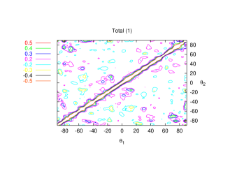
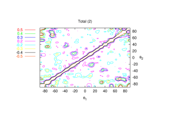
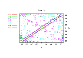
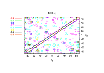
Figure 14: Contour plots of the function $C(\theta_{1},\theta_{2})$ for four realizations of the total temperature anisotropy in a toroidal universe (Sachs-Wolfe, Doppler, and ISW effects combined). The three pairs of matching circles at $\theta_{1}=-\theta_{2}=\pm 18^{\circ},\pm 39^{\circ},\pm 71^{\circ}$ are still visible despite the presence of the Doppler and integrated Sachs-Wolfe contributions.

V.2 Spherical case: lens spaces

Among the spherical spaces, the procedure presented above can be applied most easily to lens and prism spaces, because their eigenmodes are known explicitly. The eigenmodes are known analytically in toroidal coordinates (see Section III.2), and Appendix B shows how to convert them to spherical coordinates. In this section, we present some sample maps exhibiting the matching circles to demonstrate that the whole computational chain (computation of the modes and implementation in a CMB code) is working. A complete and detailed study, along the same lines as the study done for the cubic torus in the previous section, will be presented in a follow-up article.

As explained in Ref. [27], because our universe is almost flat, observational methods such as the circles method will typically detect only a cyclic subgroup of the holonomy group, so the universe “looks like a lens space” no matter what its true topology is. It follows that lens spaces are particularly interesting to capture the observational properties of multi-connected spherical spaces. In particular, we showed [27] that a cyclic factor $Z_{p}$ creates matching circles in the CMB only when $\Omega-1>1/p^{2}$ and that the second factor, if it exists, is in general undetectable.

Let us emphasize some differences with the torus case. First, concerning the eigenmodes, let us take the example of a lens space $L(p,1)$ of order $p$. For $p=1$ it reduces to ${\bf S}^{3}$ and for $p=2$ it reduces to projective space; more generally the index plays a role analogous to the size, $L$, of the torus in Euclidean space. The first non-zero eigenvalue is always $\nu=2$ and has a multiplicity $3$ for $p>2$ and $9$ otherwise. This constancy of the first eigenvalue contrasts sharply with the case of a cubic torus, for which the smallest eigenvalue scales as $L^{-1}$. It can be understood by realizing that when $p$ increases the space is becoming smaller only in one direction and remains large in perpendicular directions.

The lens spaces $L(p,1)$ are globally homogeneous (like the torus) so that the coefficients $\xi^{[{\Gamma}]\,{s}}_{{k}\,{\ell}\,{m}}$ do not depend on the observer’s position (i.e., they are the same no matter where in the space you choose the basepoint). Thus neither the correlation matrix $C_{{\ell}\,{m}}^{{\ell^{\prime}}\,{m^{\prime}}}$ nor the positions of the matching circles depend on the basepoint. Unfortunately, this is not the case for a general lens space $L(p,q)$. For a general lens space, the coefficients $\xi^{[{\Gamma}]\,{s}}_{{k}\,{\ell}\,{m}}$, the correlation matrix $C_{{\ell}\,{m}}^{{\ell^{\prime}}\,{m^{\prime}}}$ and the positions of the matching circles all depend on the observer’s position. For instance, the “canonical” choice of coordinates used in Sec. III.2.2 for the toroidal coordinate system puts the preferred symmetry axes in the $(xy)$ and $(zw)$ directions (i.e., the axis are the intersection of ${\bf S}^{3}$ with the $(x,y)$-plane and the $(z,w)$-plane, respectively, in four-dimensional Euclidean space). From a cosmological point of view, this is a poor choice, because the observer’s translated images are “atypically close”. For example in $L(12,5)$, which has cyclic factors $Z_{3}$ and $Z_{4}$, a generic observer will see three lines of four images each, but a nongeneric observer sitting on a symmetry axis will see a single line of $12$ images.

For a globally homogeneous space $L(p,1)$, the closest topological image is located at a distance $\bar{\chi}=2\pi/p$, so the topology is detectable just so $p$ isn’t too small. More precisely, the topology is potentially detectable if and only if $\pi/p<\bar{\chi}_{\scriptscriptstyle\rm LSS}$. For example, this implies that the topology is detectable for all $p>10$ if $\Omega_{\rm tot}-1\sim 10^{-2}$.

Circles match differently in a homogeneous lens space than in a tours. In a torus the circles match straight across because the holonomies are all pure translations. In a homogeneous lens space, by contrast, the holonomies are Clifford translations, and so the matching circles are still diametrically opposite but match with a twist that’s a multiple of $2\pi/p$, because Clifford translations twist and translate of the same amount.

Fig. 15 shows a CMB map with resolution $\ell_{\rm max}=30$ for the lens space $L(21,1)$ considering the Sachs-Wolfe term only. A far more detailed discussion about CMB anisotropies in lens spaces will appear elsewhere [55].

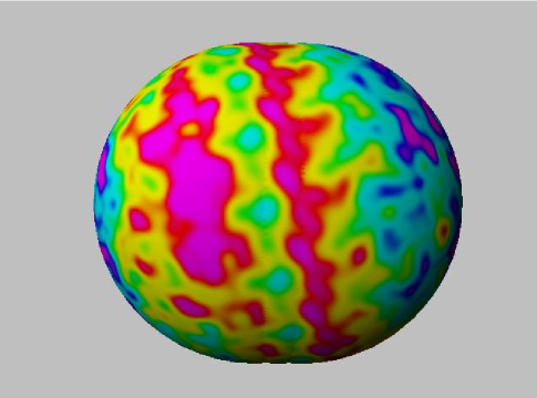
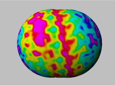
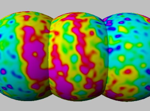
Figure 15: A realization of a CMB map in the case of the lens space $L(18,1)$. For purposes of illustration we chose a closed universe ($\Omega_{\rm tot}=1.3$) with a large last scattering surface (the radius $\chi_{LSS}$ is 0.88 times the curvature radius of the universal covering space ${\bf S}^{3}$), in order to produce higher resolution images with a large number of correlated circles. In each panel, the matching is obtained by performing a translation of $n\,R_{c}2\pi/18$ and a twist of $n\,2\pi/18$ between the last scattering surface and its two copies. The six panels correspond to $|n|=2,\dots,7$, with each panel showing both the positive ($n>0$) and negative ($n<0$) translates.

VI Discussion and conclusions

This articles describes the implementation of topology in CMB codes and gives explicitly the required tools to perform such an implementation in flat and spherical spaces. As emphasized in the Introduction, these two cases are observationally the most relevant for an almost flat universe.

Examples of simulated maps were given in the two cases. Here we presented only low resolution maps due to the computational time limitation but higher resolution maps will be presented elsewhere. It was checked that the expected topological correlations (the matched circles) were present, confirming the quality of our simulations.

Our method relies on the computation of the correlation matrix of the coefficients of the decomposition of the temperature fluctuation in spherical harmonics. This matrix encodes all the topological information. We emphasize that, due to the breakdown of global isotropy, this matrix is not purely diagonal. This also offers a working example to construct tests for the detection of deviation from global isotropy.

We have illustrated the influence of different effects that will tend to blur these patterns and affect the perfect circle matching, namely the Doppler effect and the integrated Sachs-Wolfe effect. We also considered the effect of the thickness of the last scattering surface, but found it to be negligible on the scales considered here. A more detailed quantitative analysis of these effects on the detectability of the topological signal is left for future studies [51].

A complete investigation of the detectability of the topology in coming CMB data requires the construction of reliable simulation tools. Besides the quantification of the amplitude of the effects cited above, one would also need to include all other observational effects such as instrumental noise, foreground contamination, etc. The present work paves the way to all these essential studies.

Appendix A Eigenmodes of constant curvature three-dimensional spaces

This appendix follows the work by Abbott and Schaeffer [52] and Harrison [56] and borrows heavily from Appendix A of Ref. [14]. It summarizes, without proof, the explicit forms of the scalar harmonic functions solutions of the Helmholtz equation (2).

It is convenient to factor the eigenfunctions into radial and angular functions as

$${\cal Y}^{[{X}]}_{{k}\,{\ell}\,{m}}(\chi,\theta,\varphi)=R^{[{X}]}_{{k}\,{\ell}}(\chi)Y_{\ell}^{m}(\theta,\varphi),$$ (83)

with $Y_{\ell}^{m}(\theta,\varphi)$ being the spherical harmonics. The associated eigenvalues are $\kappa_{k}^{2}=k^{2}-K$, with

$$K<0 \Rightarrow k\in[0,\infty[\quad\mbox{or}\quad ik\in[0,\sqrt{|K|}],$$ (84)

$$K=0 \Rightarrow k\in[0,\infty[,$$ (85)

$$K>0 \Rightarrow k=(\nu+1)\sqrt{K}\quad,\qquad\nu\in{\bf N}.$$ (86)

With the normalization

$$\int{\cal Y}^{[{X}]}_{{k}\,{\ell}\,{m}}(\chi,\theta,\varphi){{\cal Y}^{[{X}]}_{{k^{\prime}}\,{\ell^{\prime}}\,{m^{\prime}}}}^{*}(\chi,\theta,\varphi)\;\mbox{s}_{K}^{2}(\chi)\;{\rm d}\chi\,{\rm d}\Omega=\frac{1}{k^{2}}\delta^{{\rm D}}({k-k^{\prime}})\delta_{{\ell}\,{\ell^{\prime}}}\delta_{{m}\,{m^{\prime}}},$$ (87)

where $\mbox{s}_{K}(\chi)$ is defined in Eq. (7), the normalized radial functions take the form

$$R^{[{{\bf H}^{3}}]}_{{k}\,{\ell}}(\chi) = \left(\frac{N_{k\ell}}{k\mbox{s}_{K}(\chi)}\right)^{1/2}P_{-1/2+i\omega}^{-1/2-\ell}\left(\cosh(\sqrt{|K|}\chi)\right),$$ (88)

$$R^{[{{\bf R}^{3}}]}_{{k}\,{\ell}}(\chi) = \left(\frac{2}{\pi}\right)^{1/2}j_{\ell}(k\chi),$$ (89)

$$R^{[{{\bf S}^{3}}]}_{{k}\,{\ell}}(\chi) = \left(\frac{M_{k\ell}}{k\mbox{s}_{K}(\chi)}\right)^{1/2}P_{1/2+\nu}^{-1/2-\ell}\left(\cos(\sqrt{K}\chi)\right)$$ (90)

with

$$\omega=k/\sqrt{|K|},\qquad\nu=k/\sqrt{K}-1.$$ (91)

In the case of spatially hyperbolic spaces, this normalization is valid only for sub-curvature modes, and for the super-curvature modes ($ik\in[0,\sqrt{|K|}]$) the radial function is obtained by analytic continuation (see Ref. [57] for details). The two numerical coefficients are given by

$$N_{k\ell} \equiv \prod_{n=0}^{\ell}\left(\omega^{2}+n^{2}\right),$$ (92)

$$M_{k\ell} \equiv \prod_{n=0}^{\ell}\left((\nu+1)^{2}-n^{2}\right),\quad\quad M_{k\ell}=0\quad\mbox{if}\quad\ell>\nu.$$ (93)

For any function, we can perform the mode decomposition

$$f({\bf x})=\sum_{\ell,m}\left\{\begin{array}[]{l}\int k^{2}{\rm d}k\\ K^{3/2}\sum_{\nu=2}^{\infty}(\nu+1)^{2}\end{array}\right\}f_{k\ell m}{\cal Y}^{[{X}]}_{{k}\,{\ell}\,{m}}\,\Longleftrightarrow\,f_{k\ell m}=\int f({\bf x}){\cal Y}^{[{X}]}_{{k}\,{\ell}\,{m}}{}^{*}\sqrt{\gamma}{\rm d}^{3}{\bf x},$$ (94)

choosing the sum or the integral according to whether the universal covering space is compact or not. The symbol $\sqrt{\gamma}$ stands for the square root of the determinant of the spatial metric. In the case of spatially hyperbolic spaces, the super-curvature modes add a term to this mode expansion, namely $\int_{0}^{1}|k^{2}|{\rm d}(ik)\sum_{\ell,m}f_{k\ell m}{\cal Y}^{[{{\bf H}^{3}}]}_{{k}\,{\ell}\,{m}}$; see Ref. [57] for details.

In the spherical case, one can however find a solution of the Helmholtz equation (2) which does not involve Legendre functions. The radial part of the Helmholtz equation reduces, after setting ${\cal Y}^{[{{\bf S}^{3}}]}_{{k}\,{\ell}\,{m}}=R^{[{{\bf S}^{3}}]}_{{k}\,{\ell}}(\chi)Y_{\ell}^{m}(\theta,\varphi)$, to

$$\frac{1}{\mbox{s}_{K}^{2}(\chi)}\frac{{\rm d}}{{\rm d}\chi}\left(\mbox{s}_{K}^{2}(\chi)\frac{{\rm d}}{{\rm d}\chi}R^{[{{\bf S}^{3}}]}_{{k}\,{\ell}}\right)+\left[(k^{2}-K)-\frac{\ell(\ell+1)}{\mbox{s}_{K}^{2}(\chi)}\right]R^{[{{\bf S}^{3}}]}_{{k}\,{\ell}}=0.$$ (95)

It is obviously much more convenient to work in a coordinate system where the curvature $K$ reduces to $1$. In terms of the dimensionless radial variable $\bar{\chi}$ defined in Eq. (8), the Helmholtz equation then reduces to

$$\frac{1}{\sin^{2}\bar{\chi}}\frac{{\rm d}}{{\rm d}\bar{\chi}}\left(\sin^{2}\bar{\chi}\frac{{\rm d}}{{\rm d}\bar{\chi}}R^{[{{\bf S}^{3}}]}_{{k}\,{\ell}}\right)+\left[\nu(\nu+2)-\frac{\ell(\ell+1)}{\sin^{2}\bar{\chi}}\right]R^{[{{\bf S}^{3}}]}_{{k}\,{\ell}}=0.$$ (96)

Note that this is a second order equation and that only one of the two independent solutions is well behaved at the origin, so the radial functions are completely determined once the normalization has been chosen. After setting $R^{[{{\bf S}^{3}}]}_{{k}\,{\ell}}=(\sin\bar{\chi})^{\ell}f_{\nu\ell}$, it can be checked that it reduces to Eq. (133), the solution of which is simply given in terms of ultraspherical Gegenbauer polynomials as $f_{\nu\ell}=A_{\nu\ell}C_{\nu-\ell}^{\ell+1}$. The normalization condition (87) implies, using the integral relation (134), that

$$A_{\nu\ell}=\frac{2^{\ell+1/2}}{\nu+1}\,{\ell!}\,\sqrt{\frac{\nu+1}{\pi}}\sqrt{\frac{(\nu-\ell)!}{(\nu+\ell+1)!}}.$$ (97)

Expressing the spherical harmonics in terms of Gegenbauer polynomials by means of Eq. (131), one ends up with an expression of the eigenmodes in terms of Gegenbauer polynomials only as

$${\cal Y}^{[{{\bf S}^{3}}]}_{{k}\,{\ell}\,{m}}=A_{\nu\ell}\widetilde{A}_{\ell m}\;\;\sin^{|m|}\theta\;\sin^{\ell}\bar{\chi}\;\;C_{\nu-\ell}^{\ell+1}(\cos\bar{\chi})\;\;C_{\ell-|m|}^{|m|+1/2}(\cos\theta)\;\;{\rm e}^{im\varphi},$$ (98)

with

$$\widetilde{A}_{\ell m}=\zeta_{m}(2|m|-1)!!\,\sqrt{\frac{(2\ell+1)}{4\pi}\frac{(\ell-|m|)!}{(\ell+|m|)!}}$$ (99)

with $\zeta_{m}$ given by Eq. (132) and we used the notation $(2|m|-1)!!=(2|m|-1)(2|m|-3)\ldots 1$.

Appendix B Change of basis between toroidal and spherical coordinates

Sec. III.2.2 found the eigenmodes of lens and prism spaces in toroidal coordinates and converted them to spherical coordinates. In this appendix, we give the expression for the matrix $\alpha_{{\nu}\,{\ell}\,{m}\,{\ell_{\scriptscriptstyle{\rm T}}}\,{m_{\scriptscriptstyle{\rm T}}}}$ necessary to perform the change of basis.

The spherical coordinate system, as used in Eq. (6), is related to the embedding of the $3$-sphere ${\bf S}^{3}$ in four-dimensional Euclidean space by

$$x = \cos{\bar{\chi}},$$ (100)

$$y = \sin{\bar{\chi}}\cos{\theta},$$ (101)

$$z = \sin{\bar{\chi}}\sin{\theta}\cos{\varphi},$$ (102)

$$w = \sin{\bar{\chi}}\sin{\theta}\sin{\varphi},$$ (103)

with

$$0\leq\bar{\chi}\leq\pi,$$ (104)

$$0\leq\theta\leq\pi,$$ (105)

$$0\leq\varphi\leq 2\pi.$$ (106)

The (complex) coefficients $\alpha_{{\nu}\,{\ell}\,{m}\,{\ell_{\scriptscriptstyle{\rm T}}}\,{m_{\scriptscriptstyle{\rm T}}}}$ characterizing the change of basis are defined by

$$\alpha_{{\nu}\,{\ell}\,{m}\,{\ell_{\scriptscriptstyle{\rm T}}}\,{m_{\scriptscriptstyle{\rm T}}}}=(\nu+1)^{2}\int{\cal Q}_{{\nu}\,{\ell_{\scriptscriptstyle{\rm T}}}\,{m_{\scriptscriptstyle{\rm T}}}}(\chi_{\scriptscriptstyle{\rm T}},\theta_{\scriptscriptstyle{\rm T}},\varphi_{\scriptscriptstyle{\rm T}}){\cal Y}^{[{{\bf S}^{3}}]}_{{k}\,{\ell}\,{m}}{}^{*}(\bar{\chi},\theta,\varphi)(\sin\bar{\chi})^{2}{\rm d}\bar{\chi}\,\sin\theta{\rm d}\theta\,{\rm d}\varphi.$$ (107)

In this expression the integer $\ell$ ranges from $0$ to $\nu$ and $m$ ranges from $-\ell$ to $\ell$, while $\ell_{\scriptscriptstyle{\rm T}}$ and $m_{\scriptscriptstyle{\rm T}}$ range from $-\nu$ to $\nu$. To compute this integral, one needs:

1. to express the eigenmodes ${\cal Q}_{{\nu}\,{\ell_{\scriptscriptstyle{\rm T}}}\,{m_{\scriptscriptstyle{\rm T}}}}$ as polynomials in $x$, $y$, $z$ and $w$ (see Ref. [36]), and replace these rectangular coordinates by their expressions (100),

2. use the relations

   $$\cos^{|\ell_{\scriptscriptstyle{\rm T}}|}\chi_{\scriptscriptstyle{\rm T}}\left\{\begin{array}[]{l}\cos(|\ell_{\scriptscriptstyle{\rm T}}|\theta)\\ \sin(|\ell_{\scriptscriptstyle{\rm T}}|\theta)\end{array}\right.=\left\{\begin{array}[]{ll}\Re\left[(\cos\bar{\chi}+i\sin\bar{\chi}\cos\theta)^{|\ell_{\scriptscriptstyle{\rm T}}|}\right]&\ell_{\scriptscriptstyle{\rm T}}\geq 0,\\ \Im\left[(\cos\bar{\chi}+i\sin\bar{\chi}\cos\theta)^{|\ell_{\scriptscriptstyle{\rm T}}|}\right]&\ell_{\scriptscriptstyle{\rm T}}<0,\end{array}\right.$$ (108)

   and

   $$\sin^{|m_{\scriptscriptstyle{\rm T}}|}\chi_{\scriptscriptstyle{\rm T}}\left\{\begin{array}[]{l}\sin(|m_{\scriptscriptstyle{\rm T}}|\varphi)\\ \cos(|m_{\scriptscriptstyle{\rm T}}|\varphi)\end{array}\right.=(\sin\bar{\chi}\sin\theta)^{|m_{\scriptscriptstyle{\rm T}}|}\left\{\begin{array}[]{ll}\cos(|m_{\scriptscriptstyle{\rm T}}|\varphi)&m_{\scriptscriptstyle{\rm T}}\geq 0,\\ \sin(|m_{\scriptscriptstyle{\rm T}}|\varphi)&m_{\scriptscriptstyle{\rm T}}<0,\end{array}\right.$$ (109)

3. develop the Jacobi polynomial appearing in Eq. (57) by using Eq. (133) and with

   $$\cos 2\chi_{\scriptscriptstyle{\rm T}}-1=-2\sin^{2}\bar{\chi}\sin^{2}\theta.$$ (110)

This leads, after an easy integration on $\varphi$, to the somewhat heavy expressions involving two sums [arising from the development of the Jacobi polynomials and the power in Eq. (108)] and an integral over $\theta$ and $\bar{\chi}$,

$$\alpha_{{\nu}\,{\ell}\,{m}\,{\ell_{\scriptscriptstyle{\rm T}}}\,{m_{\scriptscriptstyle{\rm T}}}}=(\nu+1)^{2}\pi A_{\nu\ell}\widetilde{A}_{\ell m}B_{{\nu}\,{\ell_{\scriptscriptstyle{\rm T}}}\,{m_{\scriptscriptstyle{\rm T}}}}C_{{\nu}\,{\ell_{\scriptscriptstyle{\rm T}}}\,{m_{\scriptscriptstyle{\rm T}}}}\left\{\begin{array}[]{l}\Re\\ \Im\end{array}\right.\left[{\cal J}(\nu;\ell,m;\ell_{\scriptscriptstyle{\rm T}},m_{\scriptscriptstyle{\rm T}})\right]\times\left\{\begin{array}[]{l}\left(\delta_{{m}\,{|m_{\scriptscriptstyle{\rm T}}|}}+\delta_{{m}\,{-|m_{\scriptscriptstyle{\rm T}}|}}\right)\\ -i\left(\delta_{{m}\,{|m_{\scriptscriptstyle{\rm T}}|}}-\delta_{{m}\,{-|m_{\scriptscriptstyle{\rm T}}|}}\right)\\ \end{array}\right..$$ (111)

Here, the first and second line of the first brace are for $\ell_{\scriptscriptstyle{\rm T}}\geq 0$ and $\ell_{\scriptscriptstyle{\rm T}}<0$, respectively [see Eq. (108)], the first and second line of the second brace are for $m_{\scriptscriptstyle{\rm T}}\geq 0$ and $m_{\scriptscriptstyle{\rm T}}<0$, respectively [see Eq. (109)], and the numerical coefficient $C_{{\nu}\,{\ell_{\scriptscriptstyle{\rm T}}}\,{m_{\scriptscriptstyle{\rm T}}}}$ is given by

$$C_{{\nu}\,{\ell_{\scriptscriptstyle{\rm T}}}\,{m_{\scriptscriptstyle{\rm T}}}}=\frac{\Gamma(|m_{\scriptscriptstyle{\rm T}}|+d+1)}{d!\,\Gamma(|m_{\scriptscriptstyle{\rm T}}|+|\ell_{\scriptscriptstyle{\rm T}}|+d+1)}.$$ (112)

The function ${\cal J}$ is explicitly given by

$${\cal J}(\nu;\ell,m;\ell_{\scriptscriptstyle{\rm T}},m_{\scriptscriptstyle{\rm T}}) = \sum_{q=0}^{d}\left(\begin{array}[]{c}{d}\\ {q}\end{array}\right)(-1)^{q}\frac{\Gamma(|m_{\scriptscriptstyle{\rm T}}|+|\ell_{\scriptscriptstyle{\rm T}}|+d+q+1)}{\Gamma(|m_{\scriptscriptstyle{\rm T}}|+q+1)}$$ (119)

$$\times\sum_{j=0}^{|\ell_{\scriptscriptstyle{\rm T}}|}i^{j}\left(\begin{array}[]{c}{|\ell_{\scriptscriptstyle{\rm T}}|}\\ {j}\end{array}\right)I\left(j,2q+|m|+|m_{\scriptscriptstyle{\rm T}}|;\ell-|m|,|m|+\frac{1}{2}\right)$$

$$\qquad\qquad\qquad\qquad\times I\left(|\ell_{\scriptscriptstyle{\rm T}}|-j,2q+j+\ell+|m_{\scriptscriptstyle{\rm T}}|+1;\nu-\ell,\ell+1\right).$$

Note that the index $j$ is even when $\ell_{\scriptscriptstyle{\rm T}}\geq 0$ and odd when $\ell_{\scriptscriptstyle{\rm T}}<0$. This quantity involves only two sums, once the quantity $I(p,q;n,\alpha)$, defined by

$$I(p,q;n,\alpha)\equiv\int_{-1}^{1}x^{p}(1-x^{2})^{q/2}C_{n}^{\alpha}(x){\rm d}x,$$ (120)

is known. Using the expression (136) for the Gegenbauer polynomials in term of hypergeometric functions and the integral (138), it can be shown that

$$I(p,q;2m,\alpha) = \frac{(-1)^{m}}{2(\alpha+m)}\frac{B(q/2+1,(p+1)/2)}{B(\alpha,m+1)}\left[1+(-1)^{p}\right]\,{}_{3}F_{2}\left(-m,m+\alpha,\frac{p+1}{2};\frac{1}{2},\frac{q+p+3}{2};1\right),$$ (121)

$$I(p,q;2m+1,\alpha) = (-1)^{m}\frac{B(q/2+1,(p+2)/2)}{B(\alpha,m+1)}\left[1-(-1)^{p}\right]\,{}_{3}F_{2}\left(-m,m+\alpha+1,\frac{p+2}{2};\frac{3}{2},\frac{q+p+4}{2};1\right),$$ (122)

where $B$ is the Euler Beta function. It follows directly from these expressions that ${\cal J}(\nu;\ell,m;\ell_{\scriptscriptstyle{\rm T}},m_{\scriptscriptstyle{\rm T}})=0$ when $\nu-|m|+|\ell_{\scriptscriptstyle{\rm T}}|$ is odd.

Appendix C Some properties of some special functions

This appendix gathers some useful relations used in the article, to make the article more self-contained.

The spherical harmonics $Y_{\ell}^{m}$ are related to the associated Legendre polynomials $P_{\ell}^{m}$ by (see Eq. (5.2.1) of Ref. [58])

$$Y_{\ell}^{m}(\theta,\varphi)=\sqrt{\frac{2\ell+1}{4\pi}\frac{(\ell-m)!}{(\ell+m)!}}\;P_{\ell}^{m}(\cos\theta)\;{\rm e}^{im\varphi}.$$ (123)

They satisfy the conjugation relation (Eq. (5.4.1) of Ref. [58])

$$Y_{\ell}^{m}{}^{*}(\theta,\varphi)=(-1)^{m}Y_{\ell}^{-m}(\theta,\varphi)=Y_{\ell}^{m}(\theta,-\varphi),$$ (124)

the normalization (Eq. (5.6.1) of Ref. [58])

$$\int_{0}^{2\pi}{\rm d}\varphi\int_{0}^{\pi}\sin\theta\,{\rm d}\theta\;Y_{\ell}^{m}{}^{*}(\theta,\varphi)Y_{\ell^{\prime}}^{m^{\prime}}(\theta,\varphi)=\delta_{{\ell}\,{\ell^{\prime}}}\delta_{{m}\,{m^{\prime}}},$$ (125)

the closure relation (Eq. (5.2.2) of Ref. [58])

$$\sum_{\ell=0}^{\infty}\sum_{m=-\ell}^{\ell}Y_{\ell}^{m}(\theta,\varphi)Y_{\ell}^{m}{}^{*}(\theta^{\prime},\varphi^{\prime})=\delta^{{\rm D}}({\cos\theta-\cos\theta^{\prime}})\delta^{{\rm D}}({\varphi-\varphi^{\prime}}),$$ (126)

and the addition theorem (Eq. (5.17.2.9) of Ref. [58])

$$\sum_{m=-\ell}^{\ell}Y_{\ell}^{m}(\theta,\varphi)Y_{\ell}^{m}{}^{*}(\theta^{\prime},\varphi^{\prime})=\frac{2\ell+1}{4\pi}P_{\ell}(\cos\alpha),$$ (127)

where $\alpha$ is the angle between the two directions $(\theta,\varphi)$ and $(\theta^{\prime},\varphi^{\prime})$, and $P_{\ell}$ is the Legendre polynomial. The Fourier transform of the spherical harmonics is given by (Eq. (5.9.2.6) of Ref. [58])

$$\int_{0}^{\infty}r^{2}{\rm d}r\int_{0}^{2\pi}{\rm d}\varphi\int_{0}^{\pi}\sin\theta\,{\rm d}\theta\frac{{\rm e}^{i{\bf k}.{\bf r}}}{(2\pi)^{3/2}}j_{\ell}(k^{\prime}r)Y_{\ell}^{m}(\theta,\varphi)=\sqrt{\frac{2}{\pi}}i^{\ell}\frac{\delta^{{\rm D}}({k^{\prime}-k})}{k^{2}}Y_{\ell}^{m}(\theta_{\bf k},\varphi_{\bf k}),$$ (128)

where $j_{\ell}$ is a spherical Bessel function, from which it follows that (Eq. (5.17.3.14) of Ref. [58])

$${\rm e}^{i{\bf k}.{\bf r}}=\sum_{\ell=0}^{\infty}(2\ell+1)i^{\ell}j_{\ell}(kr)P_{\ell}(\cos\theta_{{\bf k},{\bf r}}),$$ (129)

and (Eq. (5.17.4.18) of Ref. [58])

$$\delta^{{\rm D}}({{\bf r}_{1}-{\bf r}_{2}})=\frac{\delta^{{\rm D}}({r_{1}-r_{2}})}{r_{1}^{2}}\sum_{\ell=0}^{\infty}\frac{2\ell+1}{4\pi}P_{\ell}(\cos\theta_{12}).$$ (130)

The spherical harmonics can also be expressed in terms of Gegenbauer polynomials as (Eq. (5.2.6.39c) of Ref. [58])

$$Y_{\ell}^{m}(\theta,\varphi)=\zeta_{m}{\rm e}^{im\varphi}\sqrt{\frac{2\ell+1}{4\pi}}\sqrt{\frac{(\ell-|m|)!}{(\ell+|m|)!}}(2|m|-1)!!(\sin\theta)^{|m|}C_{\ell-|m|}^{|m|+1/2}(\cos\theta)$$ (131)

with $\zeta_{m}$ defined by

$$\zeta_{m}=\left\{\begin{array}[]{ll}(-1)^{m}&m>0\\ 1&m\leq 0\end{array}\right..$$ (132)

The ultraspherical (or Gegenbauer) polynomials $C_{n}^{\alpha}$ are solutions of the differential equation (Eq. (22.6.5) of Ref. [59])

$$(1-x^{2})y^{\prime\prime}-(2\alpha+1)y^{\prime}+n(n+2\alpha)y=0,$$ (133)

and they satisfy the normalization condition (Eq. (7.313) of Ref. [60])

$$\int_{-1}^{1}(1-x^{2})^{\alpha-1/2}\left[C_{n}^{\alpha}(x)\right]^{2}\;{\rm d}x=\frac{\pi 2^{1-2\alpha}\Gamma(2\alpha+n)}{n!(n+\alpha)\left[\Gamma(\alpha)\right]^{2}},$$ (134)

if $\Re(\alpha)>-1/2$.

The Jacobi polynomials are given by (Eq. (22.3.2) of Ref. [59])

$$P_{n}^{({\alpha}\,,\,{\beta})}(x)=\frac{\Gamma(\alpha+n+1)}{n!\Gamma(\alpha+\beta+n+1)}\sum_{j=0}^{n}\left(\begin{array}[]{c}{n}\\ {j}\end{array}\right)\frac{\Gamma(\alpha+\beta+n+j+1)}{2^{j}\,\Gamma(\alpha+j+1)}(x-1)^{j},$$ (135)

under the conditions $\alpha>-1$ and $\beta>-1$. Interestingly, the Gegenbauer polynomials can be expressed in terms of hypergeometric functions as (Eqs. (8.932.2,8.932.3) of Ref. [60])

$$C_{2n}^{\lambda}(x) = \frac{(-1)^{n}}{(\lambda+n)B(\lambda,n+1)}\,F\left(-n,\lambda+n;1/2;x^{2}\right),$$ (136)

$$C_{2n+1}^{\lambda}(x) = \frac{(-1)^{n}}{B(\lambda,n+1)}(2x)\,F\left(-n,\lambda+n+1;3/2;x^{2}\right),$$ (137)

which satisfies the integral property (Eqs. (7.513) of Ref. [60])

$$\int_{0}^{1}x^{s-1}(1-x^{2})^{\nu}F\left(-n,a;b;x^{2}\right)\;{\rm d}x=\frac{1}{2}B(\nu+1,s/2)\;{}_{3}F_{2}\left(-n,a,s/2;b,\nu+1+s/2;1\right)$$ (138)

if $\Re(s)>0$ and $\Re(\nu)>-1$.

References

- [1] MAP homepage: http://map.gsfc.nasa.gov/ .
- [2] Planck homepage: http://astro.estec.esa.nl/Planck/ .
- [3] I.Y. Sokolov, JETP Lett. 57, 617 (1993).
- [4] A.A. Starobinsky, JETP Lett. 57, 622 (1993).
- [5] D. Stevens, D. Scott, and J. Silk, Phys. Rev. Lett. 71, 20 (1993).
- [6] A. de Oliveira-Costa and G.F. Smoot, Astrophys. J. 448, 447 (1995).
- [7] N.J. Cornish, D. Spergel, and G. Starkmann, Class. Quant. Grav. 15, 2657 (1998).
- [8] J. Levin, E. Scannapieco, G. de Gasperis, and J. Silk, Phys. Rev. D58, 123006 (1998).
- [9] K.T. Inoue, Phys. Rev. D62, 103001 (2000).
- [10] M. Lachièze-Rey and J.-P. Luminet, Phys. Rept. 254 135, (1995).
- [11] J.-P. Uzan, R. Lehoucq, and J.-P. Luminet, in XIXth Texas Symposium on Relativistic Astrophysics and Cosmology, edited by E. Aubourg, T. Montmerle, J. Paul, and P. Peter (Tellig, Châtillon, France), CD-ROM file 04/25.
- [12] J. Levin, Phys. Rept. 365, 251 (2002).
- [13] R. Lehoucq, J.-P. Uzan, and J.-P. Luminet, Astron. Astrophys. 363, 1 (2000).
- [14] R. Lehoucq, J. Weeks, J.-P. Uzan, E. Gausmann, and J.-P. Luminet, Class. Quant. Grav. 19 4683, (2002).
- [15] E. Scannapieco, J. Levin, and J. Silk, Month. Not. R. Astron. Soc. 303, 797 (1999).
- [16] K.T. Inoue, Class. Quant. Grav. 18, 1967 (2001).
- [17] R. Aurich, Astrophys. J. 524, 497 (1999).
- [18] K.T. Inoue, K. Tomita, and N. Sugiyama, Month. Not. R. Astron. Soc. 314, L21 (2000).
- [19] N.J. Cornish and D.N. Spergel, Phys. Rev. D64, 087304 (2000).
- [20] J.R. Bond, D. Pogosyan, and T. Souradeep, Class. Quant. Grav. 15, 2671 (1998).
- [21] J.R. Bond, D. Pogosyan, and T. Souradeep, Phys. Rev. D62, 043005 (2000).
- [22] J.R. Bond, D. Pogosyan, and T. Souradeep, Phys. Rev. D62, 043006 (2000).
- [23] J. L. Sievers et al., [arXiv:astro-ph/0205387]
- [24] C.B. Netterfield et al., Astrophys. J. 571, 604 (2002).
- [25] A. Benoît et al., [arXiv:astro-ph/0210306].
- [26] A. Benoît et al., [arXiv:astro-ph/0210305].
- [27] J. Weeks, R. Lehoucq and J.-P. Uzan, [arXiv:astro-ph/0209389].
- [28] G.I. Gomero, M.J. Rebouças, and R. Tavakol, Class. Quant. Grav. 18, L145 (2001).
- [29] R. Aurich and F. Steiner, Month. Not. R. Astron. Soc. 323, 1016 (2001).
- [30] K.T. Inoue, Prog. Theor. Phys. 106, 39 (2001).
- [31] G.I. Gomero, M.J. Rebouças, and R. Tavakol, Int. J. Mod. Phys. A17, 4261 (2002) [arXiv:gr-qc/0210016].
- [32] J. Weeks, “Detecting topology in a nearly flat hyperbolic universe” submitted to Int. J. Mod. Phys. A.
- [33] G.I. Gomero, M.J. Rebouças, and R. Tavakol, Class. Quant. Grav. 18, 4461 (2001).
- [34] T. Souradeep, in Cosmic Horizons, Festschrift on the sixtieth Birthday of Jayant Narlikar, edited by N. Dadhich and A. Kembhavi (Kluwer, Dordrecht, 1998).
- [35] E. Gausmann, R. Lehoucq, J.-P. Luminet, J.-P. Uzan, and J. Weeks, Class. Quant. Grav. 18, 5155 (2001).
- [36] R. Lehoucq, J.-P. Uzan, and J. Weeks, Kodai Math. Journal (in press), [arXiv:math.SP/0202072].
- [37] R. Aurich and F. Steiner, Physica D39, 169 (1989).
- [38] R. Aurich and F. Steiner, Physica D64, 185 (1993).
- [39] K.T. Inoue, Class. Quant. Grav. 16, 3071 (1999).
- [40] R. Aurich and J. Marklof, Physica D92, 101 (1996).
- [41] N.J. Cornish and D.N. Spergel, [arXiv:math.DG/9906017].
- [42] H. Kodama and M. Sasaki, Prog. Theor. Phys. Suppl. 78, 1 (1984).
- [43] V. Mukhanov, H. Feldman, and R. Brandenberger, Phys. Rept. 215, 203 (1992).
- [44] R. Durrer, Fund. Cosmic Phys. 14, 209 (1994).
- [45] W. Hu and M. White, Phys. Rev. D56, 596 (1997).
- [46] D.J. Fixsen et al., Astrophys. J. 473, 576 (1996).
- [47] J. Martin and L.P. Grishchuk, Phys. Rev. D56, 1924 (1997).
- [48] W. Hu, U. Seljak, M. White, and M. Zaldarriaga, Phys. Rev. D57, 3290 (1998).
- [49] J.P. Uzan, Phys. Rev. D58, 087301 (1998).
- [50] J.P. Uzan, Class. Quant. Grav. 15, 2711 (1998).
- [51] A. Riazuelo, R. Lehoucq, J. Weeks, J.-P. Uzan, in preparation.
- [52] L.F. Abbott and R.K. Schaeffer, Astrophys. J. 308, 546 (1986).
- [53] D.H. Lyth and E.D. Stewart, Phys. Lett. 252B, 336 (1990).
- [54] M. White and E. Bunn, Astrophys. J. 450, 477 (1995).
- [55] A. Riazuelo, R. Lehoucq, J. Weeks, J.-P. Uzan, in preparation.
- [56] E. Harrison, Rev. Mod. Phys. 39, 862 (1967).
- [57] D.H. Lyth and A. Woszczyna, Phys. Rev. D52, 3338 (1995).
- [58] D.A. Varshalovich, A.N. Moskalev, and V.K. Khersonskii, Quantum theory of angular momentum (World Scientific, Singapore, 1988).
- [59] M. Abramowitz and I.A. Stegun, Handbook of Mathematical Functions With Formulas, Graphs, and Mathematical Tables (Dover Publications, New York, 1970).
- [60] I.S. Gradshteyn and I.M. Ryzhik, Table of Integrals, series and products, (Academic Press, New York, 1980).