Time-series Spectroscopy of Pulsating sdB Stars III: Line Indices of PG 1605+072

Abstract

We present the detection and analysis of line index variations in the pulsating sdB star PG 1605+072. We have found a strong dependence of line index amplitude on Balmer line order, with high-order Balmer line amplitudes up to 10 times larger than H$\beta$. Using a simple model, we have found that the line index may not only be dependent on temperature, as is usually assumed for oscillating stars, but also on surface gravity. This information will provide another set of observables that can be used for mode identification of sdBs.

1 Introduction

Subdwarf B (sdB) stars are hot, core-helium burning stars, with hydrogen envelopes that are too thin to sustain nuclear fusion. The discovery of multimode pulsations in some sdBs should allow the use of asteroseismology to probe their atmospheres, and thereby help to answer the many questions remaining about sdB formation and evolution.

Until recently, time-series observations of pulsating sdBs have been limited to photometry. We have shown that it is possible to detect radial velocity variations of Balmer lines in the pulsating sdB star PG 1605+072 using 2 m-class telescopes (? (? ? (?, ? (?, hereafter Papers I and II). Four-metre class telescopes have also been used to detect velocity variations in sdBs (?; ?). In Paper II we found closely spaced peaks in the amplitude spectrum of PG 1605+072, as well as amplitude variation in at least one of these peaks. In this paper we describe the analysis of line-index variations of Balmer lines in PG 1605+072. The atmospheric parameters of this sdB have been determined from high-resolution optical spectra and NLTE model atmospheres to be $T_{\mathrm{eff}}$=32 300$\pm$300 K and log $g$=5.25$\pm$0.05 (?). The helium abundance was found to be subsolar, i.e., log (He/H)=$-$2.53$\pm$0.1. The star was also found to be rotating with a projected rotational velocity of 39 km s^-1.

The use of equivalent widths of Balmer lines to monitor stellar oscillations of solar-type stars was first proposed by ? (?). The Balmer lines are very temperature sensitive – the equivalent width of these lines depends on the number of hydrogen atoms in the second level. According to ? (?), the maximum line strength of H$\alpha$ to H$\delta$ is between 8500 K and 9000 K at log $g$=4.0. Since the temperature changes slightly with the oscillations, the equivalent width must also change. The idea was extended by ? (?) to include metal lines. In this paper we calculate line indices, which depend on the temperature and surface gravity sensitivity of the equivalent widths of spectral lines. This method has been used to identify modes in the $\delta$ Scuti stars FG Vir (?) and BN Cnc (?), and to detect equivalent-width oscillations in the H$\alpha$ line of the roAp star $\alpha$ Cir (?). Here we present the first detection of line index variations in a pulsating sdB star, namely PG 1605+072, and find a dramatic dependence of line-index amplitude on Balmer line number. We show that a simple model can qualitatively explain this effect as a combination of temperature and surface gravity fluctuations.

2 Observations and Reductions

In this paper we use the spectroscopic observations described in Papers I and II. Briefly, they consist of 16 nights in May 2000 using DFOSC on the Danish 1.54 m in Chile, 4 nights overlapping this using ALFOSC on the NOT 2.56 m and, to improve frequency resolution, a further $\sim$1 hour per night for a month in March–April 2000 using DFOSC. We also have 10 nights of observations using DFOSC from July 1999 using the same setup, as well as 2 nights using the coudé spectrograph mounted on the Mount Stromlo 74-inch telescope in Australia. Finally, we have 12 nights of Johnson $B$ photometry from the South African Astronomical Observatory, also taken in July 1999 (see Paper I).

As described in Papers I and II, reductions of the spectra were done using standard IRAF routines for bias subtraction, flat fielding and background light subtraction, and spectra were extracted using a variance weighting algorithm. A typical spectrum is shown in Figure 2. For details of photometric reductions see, for example, ? (?).

Figure 2: Spectrum of PG 1605+072 taken using DFOSC at the Danish 1.54 m telescope. The continuum is clear until around H$\epsilon$.

3 The Line Index

We measure the line index, a quantity which depends on the temperature and surface gravity sensitivity of the equivalent width. It is defined as

$$\Lambda^{\mathrm{L}}=\sum_{x}\frac{C_{x}-S_{x}}{C_{x}}W_{x}^{\mathrm{L}}$$ (1)

(?), where $C_{x}$ is the continuum count level at pixel $x$, $S_{x}$ is the source count level, and $W_{x}^{L}$ is a gaussian-like weighting functionfor the line in question. The value of $C_{x}$ is found using $C_{x}=\sum S_{x}W_{x}^{\mathrm{C}}/\sum W_{x}^{\mathrm{C}}$ where $W_{x}^{\mathrm{C}}$ is a broad filter function and is also gaussian-like. $W_{x}^{\mathrm{L}}$ is centered by moving an integration weight filter across the line in question. The position that maximises the sum through this filter is taken as the line centre (?). The width of the function can be chosen arbitrarily; we have chosen the approximate full width at half maximum of each Balmer line, which means we use a different filter for each line.

Prior to calculating the line index, each spectrum was normalised to an average number of counts per pixel and divided by the local continuum. The line index was calculated by multiplying each Balmer line and the adjacent continuum by the weighting function (a super-super-gaussian: $e^{-x^{8}}$), dividing the line by the average of the two continua, and then summing over the line. In this way, the line index can be thought of as similar to the Strömgren H$\beta$ index, calculated using software filters. (For a justification of the term “line index” as an analogue to a colour index, see ? (? ? (?). The software for calculating line indices has been collected in a software package called Ix, as described by ? (?).

3.1 Individual Balmer Lines

Figure 4: Line index as a function of time for the H8 line.

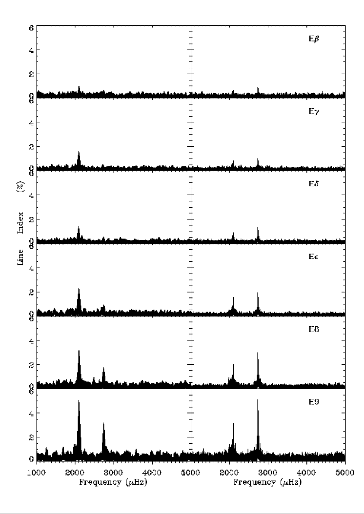
Figure 6: Line index amplitude spectra for 6 Balmer lines, from H$\beta$ at the top to H9 at the bottom. The left panels are based on July 1999 observations and the right panels on March-May 2000 observations. A dramatic increase in amplitude is evident towards higher-order Balmer lines.

We have calculated the line indices of all Balmer lines from H$\beta$ to H9. These values were normalised to a mean of zero and divided by the total mean to give the fractional change (i.e. we calculated $(\Lambda-\langle\Lambda\rangle)/\langle\Lambda\rangle$, where $\langle\Lambda\rangle$ is the mean line index). A sample line index curve (of H8) is shown in Figure 4; the peak-to-peak scatter of the best quality data (from the NOT) is around 20%. As in Papers I and II, the quality of the data varies from night to night, so we have weighted the Fourier transform using the internal scatter.

The amplitude spectra for the six Balmer lines from H$\beta$ to H9 is shown in Figure 6. The left column shows results for the 1999 data (Paper I), while the right column shows the 2000 data (Paper II). An amplitude change is evident over the 300 days between observations, similar to that seen in velocity. Also, line-index amplitudes vary strongly with Balmer line number in both sets of observations. We now consider possible reasons for the latter effect.

3.2 Dependence of amplitude of Balmer-line order

Could the variation with Balmer line order seen in Figure 6 be an artifact of our measurement technique? There are several factors we should consider.

Firstly, in sdB stars the Balmer lines are broadened by temperature and gravity, so it is difficult to measure the continuum near high-order lines ($n$=9–12), since it does not really exist in these regions. However, the amplitudes of the strongest peaks differ by about a factor of three between H$\beta$ and H$\epsilon$, and these lines have good continuum, as seen in Figure 2. Still, the wings of the Balmer lines are very broad in sdBs and are dominated by gravity effects, so we will investigate this “pseudo-continuum” at high order Balmer lines in Section 4.

A second explanation may be that the wings of the Balmer lines are oscillating out of phase with the cores. Since the wings extend out so far, they may be inadvertantly sampled as part of the continuum and thereby boost the observed amplitude of line index change. We have determined the line index variation across each Balmer line at each of the frequencies in Table 7 of Paper II. The phases at each frequency are constant when we examine different slices across the line, leading us to rule out this explanation.

4 A Simple Model

To investigate the observed behaviour, we have used H-He line blanketed, metal-free NLTE model sdB spectra (?) at log $g$=5.0, 5.25, 5.5 and $T_{\mathrm{eff}}$=30 000 K, 32 500 K and 35 000 K. The helium abundance is fixed at log (He/H)$=-2.5$. The calculations that follow were also carried out using metal line-blanketed LTE model sdB spectra with solar metallicity and Kurucz’ ATLAS6 Opacity Distribution Functions (?), but since the basic conclusions are the same, we present only the NLTE results. A detailed discussion of NLTE vs. LTE models can be found in ? (?). In the following sections we will compare the line indices of Balmer lines in these spectra with those of our observations.

4.1 The Effect of Temperature

Figure 8: Model sdB spectrum with $T_{\mathrm{eff}}$=32 500 K and log $g$=5.25, used to determine line index variations. The continuum is based on a typical NOT spectrum. Flux is in arbitrary units.

For most oscillating stars, it is usually assumed that variations are predominantly effected by temperature changes, and that radius changes (and hence surface gravity changes) are negligible (e.g., ? (? ? (?). In this case, the oscillation amplitude in line index is related to the temperature fluctuations by the relation

$$\frac{\delta\Lambda}{\Lambda}=\frac{\partial\log\Lambda}{\partial\log T}\frac{\delta T}{T}.$$ (2)

Figure 10: LTE model line index, $\Lambda$ (top panel) and its derivative $\partial\log\Lambda/\partial\log T$ (bottom panel), both as a function of effective temperature. The symbols have the following meaning: diamonds – H$\beta$; triangles – H$\gamma$; squares – H$\delta$; crosses – H$\epsilon$; open circles – H8; stars – H9; filled circles – H10.

For cool stars $\partial\log\Lambda/\partial\log T$ is positive, but for hot stars such as sdBs, it is expected to be negative. (Note that for A stars it is approximately zero). To investigate the behaviour of the line index with varying temperature for each Balmer line, we show in Figure 10 both $\Lambda$ and $\partial\log\Lambda/\partial\log T$ as a functions of temperature. Here we have used LTE models with a larger range of effective temperatures and the surface gravity fixed at $\log g$=5.5. Prior to calculating the line indices, we rebinned the model spectra to the approximate dispersion of our observed spectra and multiplied these spectra by a typical continuum from the NOT observations. We also used exactly the same parameters in our line index software for both models and observations.

Figure 10 is similar to Figure 2 of ? (?), which was made for cooler main sequence stars. An important difference is the scale of change of line index with temperature. For cool main sequence stars there is a factor of three difference over around 1000 K for H$\beta$, while for our sdB models, the difference for H$\beta$ is about a factor of two over 20 000 K. The line index of all Balmer lines except H9 and H10 seems to converge at about 40 000 K, although without modelling beyond this temperature we cannot be certain (and $\sim$40 000 K is the upper limit of the sdB regime anyway). As is expected, the change in line index with temperature is negative, that is, the line index of hotter sdBs is smaller.

To investigate the “pseudo-continuum” idea suggested in Section 3.2, we rebinned our NLTE model spectra to the approximate dispersion of our observed spectra and again multiplied the resultant spectra by a typical continuum from the NOT observations. Our goal was to use a model that was as close to the observations as possible. We calculated line indices for each of our models, once again using the same parameters as for the observations. To simulate oscillations, we took the difference between the line index of each model Balmer line at each of the different temperatures listed above. The surface gravity of the models was fixed at log $g$=5.5. The change in line index, $\Delta\Lambda$, is approximately linearly proportional to the change in temperature $\Delta T_{\mathrm{eff}}$. Because of this relationship, we can scale the line index “amplitude” to a more realistic value of $\Delta T$. We chose $\Delta T\sim 500$ K, which is an order-of-magnitude estimate based on photometric amplitudes. Finally, we normalised these differences by the line index values at 32 500 K (the approximate effective temperature of PG 1605+072), allowing us to compare fractional changes directly with our observations.

Figure 12: line index of the highest peak (2742.85 $\mu$Hz) in the 2000 amplitude spectrum compared with a simple model with temperature variations of $\sim$500 K (dashed line).

The model line-index amplitude is plotted as the dashed line in Figure 12. Also shown is the line-index amplitude of the 2742.85 $\mu$Hz peak from the March–May 2000 observations. Both model and observations show an upward trend moving to bluer wavelengths, but the amplitudes do not match. A similar result is seen for each of the other frequencies in Table 7 of Paper II. Clearly then, these unusual variations depend on more than just temperature, particularly for the higher-order Balmer lines. We now consider the effect of changing surface gravity as well as temperature.

4.2 Add Gravity and Stir

Here we assume that the relationship between change in surface gravity and change in line index is similar to Equation 2, and that we can use the simple formula

$$\frac{\delta\Lambda}{\Lambda}=\left(\frac{\delta\Lambda}{\Lambda}\right)_{T_{\mathrm{eff}}}+\left(\frac{\delta\Lambda}{\Lambda}\right)_{\mathrm{log}g}$$ (3)

to combine the effects of $T_{\mathrm{eff}}$ and log $g$. The first term on the right of Equation 3 is the line index at fixed $T_{\mathrm{eff}}$, and the second term is at fixed log $g$. This linearity assumes that the oscillations are adiabatic, which implies that $T_{\mathrm{eff}}$ and log $g$ are in phase.

Figure 14: LTE model line index, $\Lambda$ (top panel) and its derivative $\partial\log\Lambda/\partial\log g$ (bottom panel), both as a function of surface gravity. Symbols have the same meaning as Figure 10.

We show $\Lambda$ and $\partial\log\Lambda/\partial\log g$ as functions of $\log g$ in Figure 14. The important thing to note about this figure is that the line index of low-order Balmer lines stays roughly constant with $\log g$, while for the higher order lines the line index decreases dramatically. This is related to the psuedo-continuum effect discussed earlier. The implication of Figures 10 and 14 is that line index amplitudes should be highest for higher order Balmer lines, which is what we see. We can now try to quantify this effect.

Using a similar method to that used for temperature changes above, but keeping $T_{\mathrm{eff}}$ fixed at 32 500 K, we have calculated the approximate effect of changing log $g$. To fit the combination of these effects, we minimised the rms scatter of the difference between observations and the model. The best-fitting combination of the temperature and surface gravity effects is shown in Figure 16. The fit appears to be, in general, very good, although there is some discrepancy at H10. For this frequency, we find that $\Delta T\sim 372$ K and $\Delta$log $g\sim 0.047$. Whether or not these values are reasonable will be discussed in the next section.

Assuming that this method is valid, we have determined the temperature and surface gravity changes for each frequency in Table 6 of Paper II, as well as the frequencies measured from the 1999 observations (Table 5 of Paper II), and these are shown in Table 2. The velocity amplitudes derived in Paper II are shown in the last column. The uncertainties in both $\Delta T_{\mathrm{eff}}$ and $\Delta$log $g$ were found by fixing one of the $(\delta\Lambda/\Lambda)_{i}$, and changing the other until the rms increased by the mean error of the measured line index amplitudes. We have redone our calculations including the effects of rotation ($v\sin i=39$ km s^-1 for PG 1605+072; ? (? ? (?), and find that the values in Table 2 remain the same within 0.1%.

In Figure 18 we show $\Delta T$ as a function of $\Delta\mathrm{log}g$ for both sets of observations, with 1$\sigma$ error ellipses determined from linear regression. Most of the points lie on or near the straight line. The slope of the line is 8471 K dex^-1. This can be compared with future models. If there is linearity, it would be consistent with all modes having the same $l$ value. Modelling by ? (?) found 4 modes to be $l=1$ and one to be $l=2$. We have detected 4 of the 5 modes predicted by ? (?, including the mode predicted to be $l=2$ (around 2102 $\mu$Hz). In Figure 18, this mode appears to lie on the same line as the other modes. Further modelling is required to determine whether this is inconsistent with ? (?’s model.

Figure 16: Balmer line line index with frequency 2742.85 $\mu$Hz, as a function of Balmer line, compared with a simple model (dashed line). The fit shown here gives $\delta T=\sim$372 K and $\delta\mathrm{log}g=\sim$0.047.

Table 2: Changes in temperature and surface gravity for each frequency found in Paper II derived from Balmer line line indices for both 1999 and 2000 observations.

Year	Frequency	$\Delta T_{\mathrm{eff}}$	$\Delta$log $g$	$v_{\mathrm{PaperII}}$
	($\mu$Hz)	(K)		(km s-1)
2000	2742.85	372$\pm$24	0.047$\pm$0.006	7.17
	2742.47	196$\pm$13	0.028$\pm$0.004	4.45
	2102.83	161$\pm$15	0.018$\pm$0.004	3.62
	2102.48	392$\pm$24	0.042$\pm$0.006	8.47
	2101.57	116$\pm$ 7	0.011$\pm$0.002	3.40
	2075.72	205$\pm$ 9	0.023$\pm$0.002	4.27
	1985.75	98$\pm$11	0.013$\pm$0.003	4.13
	1891.01	67$\pm$11	0.009$\pm$0.003	1.99
1999	2742.63	283$\pm$14	0.051$\pm$0.004	5.80
	2102.15	560$\pm$17	0.062$\pm$0.005	11.20
	2075.29	194$\pm$ 4	0.018$\pm$0.001	2.41
	1890.98	54$\pm$16	0.003$\pm$0.004	3.14

Figure 18: $\Delta T_{\mathrm{eff}}$ as a function of $\Delta\mathrm{log}g$ for the amplitudes shown in the top section of Table 2. The error ellipses were calculated using linear regression, and show 1$\sigma$ errors. The dashed line represents a weighted least-squares fit to the data.

5 Discussion

While the model of line index oscillations we have presented here is crude, it appears to explain the observations quite well. We now must consider whether the changes in temperature and surface gravity we determined are reasonable.

5.1 Temperature Changes

We can use the Johnson $B$ photometry presented in Paper I to test the plausibility of the temperature changes we have calculated. First, we need to convert these photometric amplitudes to fractional bolometric luminosity changes. ? (?) gave the following relationship between the fractional bolometric luminosity variation $(\delta L/L)_{\mathrm{bol}}$ and the observed fractional luminosity variation $(\delta L/L)_{\lambda}$

$$\left(\frac{\delta L}{L}\right)_{\mathrm{bol}}=\left(\frac{\delta L}{L}\right)_{\lambda}\frac{\lambda}{\lambda_{\mathrm{bol}}}$$ (4)

where

$$\lambda_{\mathrm{bol}}=\frac{hc}{kT_{\mathrm{eff}}}.$$ (5)

Equation 4 is a linearised expression, assuming the star is radiating as a blackbody. We have derived the exact form of this equation, where we also allow for the radius change in the star (in PG 1605+072, assuming radial modes, the radius change is 0.1–0.9%):

$$\left(\frac{\delta L}{L}\right)_{\mathrm{bol}} = \left[\left(\frac{\delta L}{L}\right)_{\lambda}-2\frac{\delta R}{R}\right]\times$$ (6)

$$\hskip 14.22636pt\frac{\lambda}{\lambda_{\mathrm{bol}}}(1-e^{-4\lambda_{\mathrm{bol}}/\lambda})+2\frac{\delta R}{R}.$$

As an example, consider the 2102.15 $\mu$Hz mode in our 1999 data (Paper I). The radius change is $\sim$0.9% and the photometric amplitude is 3.2%, implying that $(\delta L/L)_{\mathrm{bol}}\sim$ 10%. This leads to a temperature change of $\sim$ 490 K, which is roughly consistent with the value of 560 K shown at the bottom of Table 2. The temperature changes from photometry for the other modes from Table 2 are also about the same order of magnitude as those determined from line index. We conclude from this that the temperature values we have derived are the correct order of magnitude.

5.2 Surface Gravity Variations

It is possible that we are measuring changes in the effective surface gravity rather than the true surface gravity. The effective surface gravity is a combination of the true surface gravity and other forces acting on the stellar photosphere. In order to test whether we are measuring true surface gravity variations, we have calculated the radius change expected from the best-fit variation in surface gravity at each frequency. These changes are shown in Table 4, along with the radius changes calculated from velocity amplitudes, assuming all modes are radial. The difference between the radius change for a radial and non-radial mode is a scaling factor which is dependent on the inclination angle and limb darkening. For example, with no limb darkening and with the star pole on, an $l=1,m=0$ mode will have an apparent radius change $\sim$30% larger than an $l=0$ mode with the same frequency, while an $l=2,m=0$ mode will have a radius change $\sim$10% smaller (?). ? (?) presented an analysis for solar-like stars that also considered limb darkening. They found that the mode sensitivity of the line index of Balmer lines is similar to that of Balmer-line velocity.

Table 4: Change in radius determined from log $g$ variations, compared with change in radius expected from velocities for a radial mode.

Year	Frequency	$\left(\frac{\Delta R}{R}\right)_{\mathrm{log}g}$	$\left(\frac{\Delta R}{R}\right)_{\mathrm{vel}}$
	($\mu$Hz)	(%)	(%)
2000	2742.85	5.41	0.44
	2742.47	3.22	0.27
	2102.83	2.07	0.29
	2102.48	4.84	0.68
	2101.57	1.27	0.27
	2075.72	2.65	0.35
	1985.75	1.50	0.35
	1891.01	1.04	0.18
1999	2742.63	5.87	0.36
	2102.15	7.14	0.90
	2075.29	2.07	0.20
	1890.98	0.35	0.28

All of the values of $\Delta R/R$ calculated from the log $g$ changes are larger than those calculated from velocity by at least a factor of five. A more realistic interpretation of the line index measurements requires sophisticated models. Phase dependent synthetic spectra need to be calculated that also account for limb darkening and rotation. As a prerequisite for such model spectra, the time dependent surface distribution of $\mathrm{T}_{eff}$, ${\mathrm{log}}\,g$ and the velocity field have to be determined. ? (?) has developed such a program (BRUCE) for the analysis of pulsations in rotating hot massive stars. ? (?) recently wrote a code for modelling synthetic spectra of sdB stars from BRUCE output which shall be used to analyse the line index variations. A much larger data set has been acquired in May/June 2002 by spectroscopic and photometric multi-site campaign which became known as the Multi-site spectroscopic telescope (MSST, ? (? ? (?). We will use the more detailed modelling when we shall analyse this much larger data set.

However we may also have to check the validity of the hydrostatic approximation. ? (?) encountered a similar problem in the analysis of the extreme helium star V652 Her; for this radially pulsating star the discrepancy between radii derived from surface gravity and spectrophotometry is about a factor of two. They found that at least for 10% of the pulsation cycle of this star the assumption of hydrostatic equilibrium is not valid, due to shocks moving through the atmosphere. For PG 1605+072 the speed of sound is more than twice as large as for V652 Her due to its different chemical composition. A study of such effects are beyond the scope of this paper and should be done after the more detailed hydrostatic spectral analysis outlined above has been carried out.

6 Conclusions

We have detected line index variations in the pulsating sdB star PG 1605+072. There is a strong dependence of line-index oscillation amplitude on Balmer line. We have developed a simple model, assuming hydrostatic equilibrium, where we use model spectra at as close to the same resolution and sampling of the observations as possible. Using this model, we have shown that despite not measuring true equivalent width variations, we can use the observables to infer effective temperature and effective surface gravity variations in PG 1605+072.

Using more detailed models, we should be able to measure the $\Delta T$ and $\Delta$log $g$ independently of photometry and velocity measurements. With this information, we will have another set of amplitudes which we can use for mode identification of sdB stars.

The authors would like to thank Mike Ireland for helpful discussions on error ellipses, and Steve Kawaler for continuing fruitful discussions on sdB evolution and interiors. This work was supported by an Australian Postgraduate Award (SJOT), the Australian Research Council, the Danish National Science Research Council through its Center for Ground-based Observational Astronomy, and the Danish National Research Foundation through its establishment of the Theoretical Astrophysics Center.

References

- 1 [ ] Baldry, I. K., Viskum, M., Bedding, T. R., Kjeldsen, H., & Frandsen, S., 1999, MNRAS, 302, 381
- 2
- 3 [ ] Bedding, T. R., Kjeldsen, H., Reetz, J., & Barbuy, B., 1996, MNRAS, 280, 1155
- 4
- 5 [ ] Christensen-Dalsgaard, J., 1994, Lecture Notes on Stellar Oscillations, Institut for Fysik og Astronomi, Aarhus Universitet, third edition
- 6
- 7 [ ] Dall, T. H., 2000. In: Bergvall, N., Takalo, L. O., & Piirola, V. (eds.), The NOT in the 2000’s. Proc. of the workshop held on La Palma, April 12-15, 2000
- 8
- 9 [ ] Dall, T. H., Frandsen, S., Lehmann, H., Anupama, G. C., Kambe, E., Handler, G., Kawanomoto, S., Watanabe, E., Fukata, M., Nagae, T., & Horner, S., 2002, A&A, 385, 921
- 10
- 11 [ ] Falter, S., 2001, Diploma Thesis (University of Erlangen-Nürnberg)
- 12
- 13 [ ] Heber, U., Dreizler, S., Schuh, S. L., & O’Toole, S. J.
- 14
- 15 [ ] Heber, U., Reid, I. N., & Werner, K., 1999, A&A, 348, L25
- 16
- 17 [ ] Heber, U., Reid, I. N., & Werner, K., 2000, A&A, 363, 198
- 18
- 19 [ ] Jeffery, C. S., & Pollacco, D., 2000, MNRAS, 318, 974
- 20
- 21 [ ] Jeffery, C. S., Woolf, V. M., & Pollacco, D. L., 2001, A&A, 376, 497
- 22
- 23 [ ] Kawaler, S. D., 1999. In: Solheim, J. E., & Meistas, E. G. (eds.), 11th. European Workshop on White Dwarfs, Vol. 169, p. 158, ASP Conference Series
- 24
- 25 [ ] Kjeldsen, H., & Bedding, T. R., 1995, A&A, 293, 87
- 26
- 27 [ ] Kjeldsen, H., Bedding, T. R., Viskum, M., & Frandsen, S., 1995, AJ, 109, 1313
- 28
- 29 [ ] Koen, C., Kilkenny, D., O’Donoghue, D., Van Wyk, F., & Stobie, R. S., 1997, MNRAS, 285, 645
- 30
- 31 [ ] Kurucz, R. L., 1979, ApJS, 40, 1
- 32
- 33 [ ] Napiwotzki, R., 1997, A&A, 322, 256
- 34
- 35 [ ] O’Toole, S. J., Bedding, T. R., Kjeldsen, H., Teixeira, T. C., Roberts, G., van Wyk, F., Kilkenny, D., D’Cruz, N., & Baldry, I. K., 2000, ApJ, 537, L53
- 36
- 37 [ ] O’Toole, S. J., Bedding, T. R., Kjeldsen, H., Dall, T., & Stello, D., 2002, MNRAS, 334, 471
- 38
- 39 [ ] Townsend, R. H. D., 1997, MNRAS, 284, 839
- 40
- 41 [ ] Viskum, M., Kjeldsen, H., Bedding, T. R., Dall, T. H., Baldry, I. K., Bruntt, H., & Frandsen, S., 1998, A&A, 335, 549
- 42
- 43 [ ] Woolf, V. M., Jeffery, C. S., & Pollacco, D. L., 2002, MNRAS, 329, 497
- 44