Spectrophotometry with a transmission grating
for detecting faint occultations

Abstract

High-precision spectrophotometry is highly desirable in detecting and characterizing close-in extrasolar planets to learn about their makeup and temperature. For such a goal, a modest-size telescope with a simple low-resolution spectroscopic instrument is potentially as good or better than a complex general purpose spectrograph since calibration and removal of systematic errors is expected to dominate. We use a transmission grating placed in front of an imaging CCD camera on Steward Observatory’s Kuiper 1.5 m telescope to provide a high signal-to-noise, low dispersion visible spectrum of the star HD 209458. We attempt to detect the reflected light signal from the extra-solar planet HD 209458b by differencing the signal just before and after secondary occultation. We present a simple data reduction method and explore the limits of ground based low-dispersion spectrophotometry with a diffraction grating. Reflected light detection levels of 0.1% are achievable for $5000-7000$ Å, too coarse for useful limits on ESPs but potentially useful for determining spectra of short-period binary systems with large $(\Delta m_{vis}=6)$ brightness ratios. Limits on the precison are set by variations in atmospheric seeing in the low-resolution spectrum. Calibration of this effect can be carried out by measurement of atmospheric parameters from the observations themselves, which may allow the precision to be limited by the noise due to photon statistics and atmospheric scintillation effects.

1 Introduction

The indirect detection of large hot Jupiter-like extrasolar planets with periods on the order of days raises the possibility of direct detection of the reflected light from the planet’s atmosphere. The expected contrast ratio for these close-in gas giant planets is expected to be quite favorable $(10^{4}-10^{5})$ compared to the contrast ratio between Jupiter and our sun $(10^{9})$. However, the close proximity of these planets to their stars precludes spatially resolving the planet with current telescopes. Thus additional information about these planets requires other methods of discerning its flux in the presence of the much brighter star. Several approaches are possible to separate the starlight from the planet’s light. Charbonneau et al. (1999) and Collier-Cameron et al. (1999) each observed tau Boo with a high resolution spectrometer in an attempt to discern the planet’s light through by the Doppler shift of the reflected light as the planet orbits its star. Although no detection was observed, the data were sufficient to place upper limits on the planet’s albedo.

The discovery that the planet around HD 209458 occulted its star during the 3.5 day orbit (Charbonneau et al., 2000) was a significant step in verifying the existence of the extrasolar planet candidates. Brown et al. (2001) followed up this initial detection with high precision HST photometric measurements of the transit. This yielded a more precise light curve of the occultation, and gave the first indication of the composition of the planet’s atmosphere. The transit was detected to be slightly deeper at the wavelength of sodium absorption (Charbonneau et al., 2002), as predicted by various groups (Brown, 2001; Seager & Sasselov, 2000; Hubbard et al., 2001).

Direct detection of the reflected light from a close-in planet has the potential of telling us the albedo of a planet, and thus also, the temperature of the planet. From a more pedestrian viewpoint detection of the planet’s reflected light would be the indication of what the planet “looks” like. The color is more than just a curiosity, though, allowing the first constraints on the planet’s chemical makeup and vertical structure (such as the existence of clouds).

We observe the HD209458 system just before and after the eclipse of the planet by its parent star. Theoretical models suggest the planet may have a bright (0.7) albedo with a wide ($R/\Delta R\sim 20$) absorption feature due to pressure broadened sodium at 591 nm (Sudarksy et al., 2000). The reflected light fraction from the star is $2\times 10^{-4}$ for a geometric albedo of one, so a detection level of $\simeq 1\times 10^{-4}$ per wavelength band is needed to produce a useful constraint on the albedo of the planet.

Colour information is obtained with the use of a transmission grating in front of a CCD detector, in an objective prism configuration. Objective prism surveys are used with wide field imaging telescopes for spectral typing of stars and classifications of the brighter galaxies. The low dispersion, high throughput and no slit jaw losses make the objective prism method suitable for colour dependent transits. The main challenge is then in obtaining accurate spectrophotometry with the variation in transmission of the atmosphere as a function of airmass and the variation of spectral resolution due to the local seeing at the telescope.

2 Observations

All our observations were taken at the Kuiper telescope on Mount Bigelow, North of Tucson, a 1.54 m reflecting telescope with a CCD camera mounted at the Cassegrain focus.

The grating is a 72 lines/mm epoxy layer stamped onto glass $24\times 24\times 3$mm, manufactured by Edmunds Scientific. The ruling is blazed to give maximum transmission ($32\%$) in the first order. The grating is placed in the camera filter wheel approximately 10 cm from the detector.

The CCD is an unthinned $2048^{2}$ pixel detector manufactured by the University of Arizona Imaging Technology Laboratory. The camera scale is 0.15 arcseconds per pixel and the unbinned spectral dispersion of the transmission grating at 5000Å is approximately 20Å/pixel. We on-chip bin the CCD to 3 by 3 pixels, to maximize the readout rate of the detector, while still retaining the full spatial and spectral resolution for the typically 1 arcsec images at the Kuiper telescope. The distance between the grating and detector results in a spectral resolution of 39 at 5000A in 1 arcsecond seeing. Exposures were set at 5 seconds to give a peak flux integration of 50,000 ADUs, to keep the detector in a linear response range and to avoid going out of range on the 16 bit analog-to-digital converter for the CCD.

The secondary eclipse of the planet lasts three hours, with a period of just over 3.5 days (Brown et al., 2001). The data presented are from 12 November 2001 UT, which was a calm photometric night during which the secondary eclipse started soon after the star crossed the meridian (see Table 1). Over 600, five second frames of HD 209458 were acquired as the star began setting, going from airmass 1.03 to 3.0 during the observations (see Figure 1). Approximately equal numbers of frames were obtained of the star in and out of secondary eclipse. For all observations the telescope was manually guided to keep the spectrum in approximately the same part of the CCD. This number was reduced to 575 after rejection of frames where the flux of Star 1 (discussed later) showed a significant drop, most likely due to thin cloud passing overhead late in the evening.

3 Throughput

An observation of a WD primary spectrophotometric standard GD 71 (Bohlin et al., 1995) provides an estimation of the throughput of the instrument. The spectrum of the standard star is corrected to an airmass of one, and Figure 2 gives the estimated total throughput from above the atmosphere through to counts in the detector. The estimated contributions to the throughput are presented in Table 3. The dominant errors for the calculation are from the uncertainty in the gain factor for the CCD.

4 Colour response of the pixels

The gain ,$g$, of modern CCDs is assumed to be a function of pixel position $x,y$ and of wavelength $\lambda$, making $g=g(x,y,\lambda)$. In imaging the assumption is that the gain is achromatic ($g(x,y,\lambda)=g(x,y)$) for a given fixed passband. A spectrograph uses a dispersing element to convert wavelength into spatial position on the detector, i.e. $g=g(x,y,\lambda(x,y))$ where $\lambda(x,y)$ is a well defined function fixed by the position of the dispersing element and the entrance slit.

Objective grating spectroscopy lies between these two extremes. The “entrance slit” is defined by the position and image size of the object in the sky, and any image motion of the object results in a motion of its spectrum on the CCD. This means that $\lambda(x,y)$ is not a well-defined function. Without a slit in the system we need to apply a gain correction which is based on white light illumination and assume this is valid for the range of wavelengths observed with the grating.

To see if our assumption of an achromatic gain ($g(x,y,\lambda)=g(x,y)$) is valid for our CCD we took two sets of flat fields with different colours, one with the telescope dome open and the telescope pointing to the morning twilight sky (a predominantly blue colour) and the other with the dome closed and tungsten lights switched on (a 3000 K blackbody) and pointing at the dome ceiling. Both sets were taken with the filter wheel rotated to the “clear” slot.

For the twilight (sky) flats, frames with mean counts above 50000 or lower than 10000 were rejected, along with any that have an exposure time shorter than 2 seconds, to prevent illumination gradients due to the finite shutter speed. For the tungsten lamp (dome) flats, a set of 114 exposures were taken with a mean count level of 50,000. For both sky and dome flats, the individual frames are scaled individually by their respective modes and then combined as an average with avsigclip rejection.

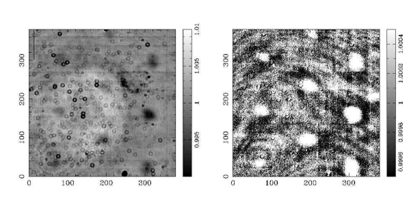
Figure 3: The Dome flat field is shown in the left-hand image, and the dome flat divided by the sky flat is shown in the right-hand image. The region of the CCD that images the spectrum shows no significant variations between sky and dome illumination above the noise in the two frames, indicating that the gain for the detector is achromatic and either frame can be used for gain correction of the spectrum.

The two flat fields are processed by MKSKYFLAT to remove large scale illumination effects. Both flats show CCD manufacturing imperfections and ’mirror donuts’ symptomatic of dust on the dewar window surfaces, and dividing the dome flat by the sky flat removes virtually all the larger dust artefacts (see left-hand of Figure 3). Given the quoted gain of $3.2\pm 0.1e^{-}/\rm{ADU}$ for the CCD the statistics shown in table 2 are consistent with photon shot noise being the dominant source of noise in the combined flats.

Dividing the dome flat into the sky flat produces the image shown in the right-hand side of Figure 3. The residual artefacts are a triangularly spaced set of higher-gain spots, and some fringing that is just visible in the noise of the image. The spots are thought to be where adhesive holds the CCD in its protective housing, and the fringes are variations in the doping applied in the manufacturing process of the CCD.

Measuring the fractional noise in flat regions of this image gives a value of $9.0\pm 1.0\times 10^{-4}$, consistent with the noise level of $8.17\pm 1.56\times 10^{-4}$ expected when dividing the sky flat into the dome flat. This image shows that, apart from some obvious regions of the CCD which can be avoided, both the sky flat and dome flat agree with each other within errors. The lack of any major gradient across the CCD means that $g(x,y,\lambda)=g(x,y)$ is valid to within measurable errors and the flat with the higher S/N ratio can be used without introducing any colour biased systematic noise into the data. We can therefore use a “white light” flat to correct for gain variations over the whole spectrum.

5 Data Reduction

5.1 Frame reduction

The data were reduced with the IRAF data reduction tasks. 100 zero frames are combined with the CCDPROC task using the ccdclip rejection for removing outlying events, and this combined zero frame is subtracted from the data. The data is then trimmed to remove the bias and overscan regions of the CCD.

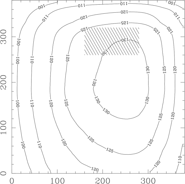
Figure 4: Contour plot of the sky background flux. The sky background is not uniform due to the vignetting of the grating. The contours show light levels after the image is median smoothed. The hatched region indicates the location of the spectra. North is up and East to the left.

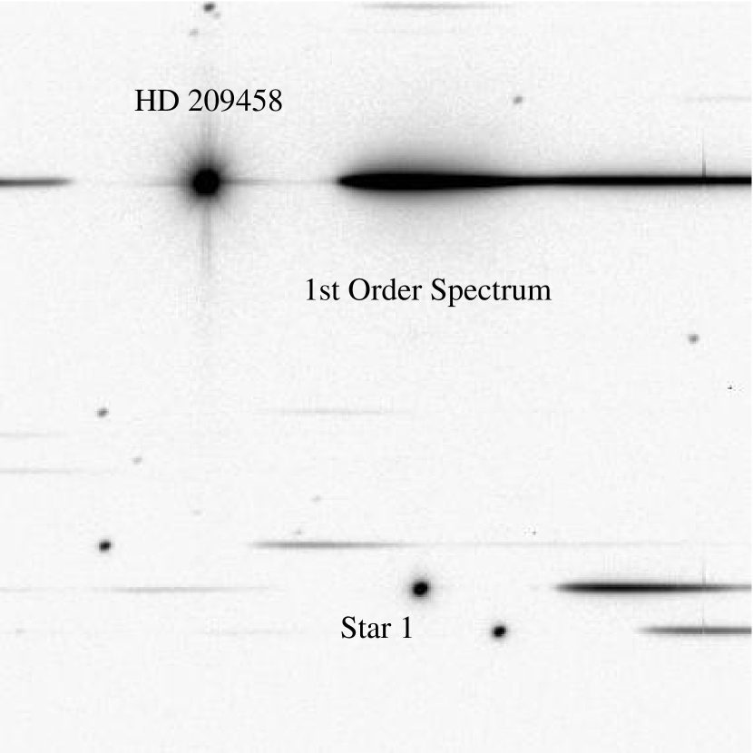
Figure 5: A typical data frame showing the positions of HD 209458 and the star used in estimating the scintillation noise. North is up and East to the left.

The data frames are flat-fielded using a gain map constructed from the dome flat field described in the previous section. The grating creates a non-uniform illumination pattern across the detector, due to vignetting of the incoming light. To remove this a sky background frame is generated by combining 100 frames taken with the telescope drive switched off. These frames are median scaled and median combined with the ccdclip rejection algorithm. The resulting image is filtered with a boxcar median filter 51 pixels to a side to smooth out high spatial frequency noise (see Figure 4). Differencing this smoothed image from the unsmoothed original shows no remaining large scale variations in the sky background image. This sky background frame is then scaled to a blank region of the CCD and subtracted on a per frame basis. Bad columns and hot pixels are replaced by interpolation from the nearest neighbouring pixel values with FIXPIX (see Figure 5).

The plate scale is determined from the position of three stars in the field of view from an image taken at an airmass of 1.03. Centroid fitting for each of the stars is performed, and the relative separations of the stars are taken from the astrometric solution attached to the DSS image covering the region around HD 209458. The plate scale is calculated to be $0.4314\pm 0.0015\arcsec/\rm{pix}$.

We use the three brightest stars in the frame to provide registration between the frames. The IRAF routine IMCENTROID gives the frame offset relative to the first frame of the night.

The total range of image motion is (8.5,5.8) pixels in the (RA,dec) axes, with typical (RMS) shift of $\delta RA_{rms}=1.119,\delta dec_{rms}=0.823$ pixels, less than the typical seeing disk size of 3 pixels (1 arcsecond). The larger drift in the RA axis is thought to be due to periodic corrections in the siderial rate applied by the telescope guidance computer when a certain drift limit is exceeded.

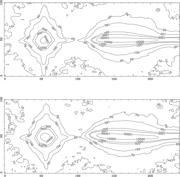
Figure 6: Scattered light from the grating. The zeroth order image and first order spectrum are seen. These images have been smoothed with a Gaussian and are in units of photons. The upper image is from airmass 1.03, the lower image taken at an airmass of 2.7. Both have had the sky background and detector bias levels subtracted. North is up and East to the left.

The remaining sources of light are the zeroth order images, the first and second order spectra from the grating, and a halo of scattered light surrounding the spectra themselves. A typical sky background subtracted image is shown in Figure 6, with a contour plot showing the scattered light profile around the spectrum. As can be seen in Figure 6, the scattered light around the spectrum is constant for images at the beginning and end of the night, indicating it does not effect our measurement of the light in the core of the spectrum in a systematic way.

5.2 Spectrum extraction and calibration

Using the centroid of Star 1 as a fiducial, a box is drawn around and centered on the first order spectrum, where the columns are perpendicular to the dispersion axis of the grating. A Gaussian curve is fit along each column to measure the PSF of the grating at that wavelength and to trace the centroid of the spectrum across the CCD. A low-order polynomial is fit to both the measured FWHM and centroid positions (see Figure 7). The RMS between the FWHM fit and data is $1.48\times 10^{-2}$ pixels for all frames during the evening. A plot of the transverse FWHM at 7000Å  as a function of Frame Number (Figure 8) shows that the seeing varies on timescales of seconds, minutes and hours during the observations.

The counts within each column are summed to give a one-dimensional spectrum with flux per wavelength bin. The width of the box is set at 41 pixels (17 arcsec), extending well into the scattered light region from the grating. Increasing the extraction width of the box does not change the extracted planetary spectrum, implying that our assumption about the scattered light is valid.

The wavelength zero point is determined from the position of atmospheric absorption due to the Fraunhofer A band of Oxygen (hereafter referred to as the ’notch’) at 7620 Angstroms. Measuring the notch pixel position with respect to the zeroth order image of the star is performed by fitting a gaussian to the notch in the extracted spectrum. The position of the notch is expected to smoothly change with airmass during the night, and so we take the fitted value of the notch position to be our wavelength zero point. Figure 9 shows the centroid of the notch as a function of frame number and the residuals after taking off a linear fit in effective airmass $a$. The RMS between the centroid fit and measured centroid of the notch is $6.0\times 10^{-2}$ pixels. Assuming that the measured notch centroids are independent of each other, the mean centroid error is reduced by the square root of the number of frames used in the notch fit. This gives a mean notch centroid error of $6.0\times 10^{-2}/\surd{573}=2.5\times 10^{-4}$ pixels ( $3.5\times 10^{-2}$Å).

As the star moves from the zenith an extra component of dispersion due to colour-dependent refraction in the the Earth’s atmosphere is added to the dispersion of the grating and the wavelength solution changes smoothly and continuously throughout the night. This atmospheric dispersion adds vectorially to the transmission grating dispersion to produce the observed wavelength solution on a given frame.

At the zenith, the grating is assumed to have a low-order polynomial wavelength solution where distance from the zeroth order image is monotonic with wavelength. A planetary nebula (PNe) of small angular extent (IC 2165) is observed and provides wavelength calibration for the extracted spectrum in the form of emission lines of $\rm H\alpha$ and O[III]. This observation was taken at a high airmass, and so the line positions are corrected using an atmospheric refraction model back to the zenith. We use a model of atmospheric refracton for the Earth’s atmosphere from Filippenko (1982), taking estimated values for the temperature and pressure from the observatory log sheets. The PNe wavelength data is corrected back to the zenith, and the resultant dispersion solution is linear within measuring errors, implying that the grating dispersion is linear with wavelength.

Using the wavelength solution for the grating and the vector correction for dispersion in the atmosphere at the required airmass, the spectra are resampled using cubic spline interpolation into $50$Å wavelength bins from $4000-8000$Å. This spectral range is limited by the efficiency of the detector in the blue end of the spectrum, and the second order spectrum appearing beyond $8000$Å.

6 The Atmospheric Model

For a single observed stellar spectrum $I(a,\lambda)$ as observed from the ground at effective airmass $a$, we assume an atmospheric model of the form:

$$I(a,\lambda)=I(\lambda).e^{-a.\tau(\lambda)}$$ (1)

where $I(\lambda)$ is the stellar spectrum for an effective airmass of zero, i.e. above the atmosphere, and $\tau(\lambda)$ is the atmospheric absorption.

For an eclisping binary at secondary eclipse, the unobscured fraction of the secondary’s disk varies from 1 at first contact to 0 at second contact, remaining at 0 until it emerges from behind the primary at third contact and rising up to 1 at fourth contact. This function is represented as $p(t)$. For the geometry of the HD 209458 system, the reflected light also varies as the phase of the planet varies, but the $p(t)$ is a good approximation to the actual phase for our data set.

The usual definition of $a=\sec z$ holds true for a semi-infinite plane-parallel atomsphere. We keep the semi-infinite atmosphere and take account of the curvature of the Earth. A simple function relates the zenith distance $z$ of the star to an effective airmass $a$:

$$a_{eff}=\frac{R}{r}.\left(\sqrt{\cos^{2}z+2.\left(\frac{r}{R}\right)+\left(\frac{r}{R}\right)^{2}}-\cos z\right)$$ (2)

Where the radius of the Earth is $R=6378\rm{km}$ and the height of a homogeneous atmoshpere (finite height, constant temperature equal to the surface temperature and constant density equal to surface density) at 15 Celsius is $r=8.43\rm{km}$ (Cox et al., 1999). Using equation 2 we calculate the effective airmass as a function of time.

Given knowledge of the ingress and egress times for an eclipsing binary system and the geometry of the system, a model for the secondary eclipse as observed on the ground is constructed:

$$I(a,t,\lambda)=I(\lambda).[1+f(\lambda).p(t)]e^{-a(t).\tau(\lambda)}$$ (3)

Here we define $f(\lambda)$, the ratio of the secondary’s spectrum to that of the primary star. For reflected light from an ESP, this is proportional to the planet’s albedo.

Taking the logarithm of this equation and realising that $\ln(1+x)\simeq x$ for $x\ll 1$ gives:

$$\ln I(a,t,\lambda)=\ln I(\lambda)+f(\lambda).p(t)-a(t).\tau(\lambda)$$

This linear equation is then fitted numerically with linear methods to produce estimates of $I,f,\tau$. Errors on each of the free parameters are estimated by simulating data for the star system assuming limitations due to Poisson distributed noise. For a given set of $I_{0}$, $\tau_{0}$, and $f_{0}$ at a particular wavelength, an ideal noiseless $I(a)$ is constructed and noise commensurate with our observations is added. The noise is estimated by taking the r.m.s. of the difference of the fitted light curve and the actual data. A linear fitting routine then extracts “measured” values of $I,\tau,f$. Repeating this process with a different sample of Poisson noise produces distributions of $I_{m}\pm\delta I,\tau_{m}\pm\delta\tau,f_{m}\pm\delta f$, where the $\delta-$ quantities correspond to 1-sigma limits of the resultant Poisson distributions, and these are the error bars on our results.

Figure 10 and 11 show the fitted spectrum of HD 209458 and the derived extinction curve of the atmosphere. The derived spectrum for the planet HD 209458b is shown in Figure 12. The mean planet flux over the passband 5000-7000Å is $-7.0\pm 8.4\times 10^{-4}$, the sensitivity of which is approximately 4 times larger than the maximum reflected light fraction of $2\times 10^{-4}$.

Using our model of the atmosphere we construct a set of model spectra for the measured range of airmass $a(t)$ and planet phase $p(t)$. For $I(\lambda)$ and $\tau(\lambda)$ we use the values derived in the extraction of HD 209458 and we assume a constant reflected light fraction $f(\lambda)=2\times 10^{-4}$. Adding only photon shot noise results in an extracted spectrum as shown in Figure 13. The measured planet flux is detected with a level of $(2.0\pm 1.8)\times 10^{-4}$ per 50Å bin. Averaged over the 40 bins in the range of 5000-7000Å this results in an accuracy of $2.8\times 10^{-5}$ in the limit of photon noise.

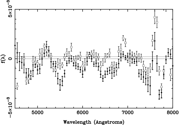
Figure 15: Simulated and actual extracted model planet spectrum for ideal atmosphere with photon noise, scintillation noise and atmospheric blurring. Circles are the actual data, and white squares are the simulated data. The dominant effect appears to be from variable atmospheric blurring of the spectrum.

Making the assumption that the PSF along the spectra is the same as the PSF measured across the spectrum, we apply atmospheric seeing effects to the data set. The extracted planetary spectrum (Figure 14) shows a significant systematic error similiar in sign and magnitude to that seen in our measured data. Our exposure times are short enough that we are also affected by scintillation noise and including this contribution produces the spectrum shown in Figure 15.

A simulated spectrum can be created with no planetary signal which has the same systematic errors as the actual data, as shown in Figure 15. This can be used to normalise the signal detected in the data. We create a normalised spectrum $f_{norm}(\lambda)$ with:

$$f_{norm}(\lambda)=\frac{1+f_{meas}}{1+f_{model}}$$

where $f_{meas}$ is our observed planet spectrum, and $f_{model}$ is the simulated planet spectrum.

The resultant spectrum in Figure 16 shows a reduction in systematic effects and gives a mean fractional planet flux of $-8.2\pm 6.2\times 10^{-4}$ averaged over the bandpass of 5000-7000Å.

7 Limits to the Precision

The fundamental limit to the precision of the photometric measurement in each wavelength bin is set by the number of photons collected. The uncertainty in the intensity is governed by Poisson statistics, and is thus given by the square root of the photons collected per wavelength bin per exposure. As can be seen in Figure 10 the peak flux per exposure per 50Å wavelength bin at an airmass of zero is approximately $4.0\times 10^{5}$ photons for most of the 5000-7000Å portion of the spectrum. Taking into account the absorption of the atmosphere averaged over the night, this figure lowers to $3.5\times 10^{5}$ photons, creating an uncertainty of $1.69\times 10^{-3}$ in the intensity. However, no correlation exists between wavelength bins or exposures, allowing this uncertainty to be reduced. For the 240 exposures taken while the planet was eclipsed by the star, and the 200 taken when the planet was not, these give uncertainties of $1.12\times 10^{-4}$ and $1.09\times 10^{-4}$ which when combined in quadrature give a photon-limted uncertainty per wavelength bin of $1.56\times 10^{-4}$, comparable to the $1.8\times 10^{-4}$ from the photon-limited model in the previous section.

The measured variations in intensity per frame are also expected to be affected by scintillation of the starlight. Young (1967) derived the variations in intensity due to scintillation. The uncertainty in intensity for typical scintillation is given by the equation

$$\sigma=S_{0}.D^{-2/3}(\sec Z)^{1.75}e^{-h/h_{0}}/(t)^{1/2}$$

where $D$ is the telescope aperture in meters, $t$ is the exposure time in seconds, $Z$ is the zenith angle, $h$ is the height of the observatory (2.5 km for the Kuiper telescope), and $h_{0}$ is the turbulence weighted atmospheric altitude (typically 8 km). $S_{0}$ is the normalization constant for the effect, which is typically 0.003, but can vary due to the strength and height of the turbulence. Work by Dravins et al. (1998) have verified this equation for various timescales and aperture sizes, showing that the strength of scintillation varies (as parameterized by $S_{0}$ in the equation above) and is not well correlated with the local seeing. For the 5 second frames, at airmass 1.5 each frame would have a variation of 1.5$\times 10^{-3}$. As indicated by the square root dependence on exposure time, successive images are not correlated. Thus for the 240 exposures taken while the planet was eclipsed by the star we expect the scintillation-induced uncertainty per wavelength bin to be 1.3$\times 10^{-4}$. However, studies by Dravins et al. (1997) and Ryan & Sandler (1998) do show that the the effects of scintillation can be considered achromatic in their effect on a spectrum. That is, the variations in intensity are correlated between wavelength bins.

The value of $S_{0}$ changes significantly between nights and observing sites (Dravins et al., 1997), and so we use the measured flux of Star 1 to determine the value of this scintillation constant for our data. We calculate the flux of Star 1 as a fuction of airmass and fit an exponential curve to the data, assuming a single value for $\tau$. From our observed data, we know that $\tau$ changes as a function of wavelength, and the difference of the fit and the data show this as a low-order residual with a peak of approximately 0.5% of star 1’s flux at 1 airmass. A low-order curve is fitted to remove this remaining flux, and for each observed value of the star 1’s flux, an estimate of the poisson noise and the scintillation noise is made (see Figure 17). The scintillation coefficient that best fits the scatter in star 1’s flux is $0.006\pm 0.002$, and the short-term variations in the flux are attributed to variations in $S_{0}$ during the night. This corresponds to a scintillation-induced uncertainty of approximately $3\times 10^{-3}$ per frame or 2.6$\times 10^{-4}$ over the transit of the planet.

As can be seen by the comparison of photon and scintillation noise, for nominal scintillation the spectral resolution is appropriate for nearly equal noise contributions from each. Higher spectral resolution would cause photon noise to dominate for each wavelength bin, while lower resolution would cause scintillation noise to dominate. Thus a spectral resolution of 30-60 is suitable for balancing these two sources of error. The photon noise scales inversely with the diameter of the telescope while the scintillation scales inversely as the 2/3 power of the diameter. In general this means that the optimum resolution for balancing these sources of noise (for HD 209458) is given by $R_{opt}\sim 30\times D^{1/3}$ where D is the telescope diameter in meters. This suggests that even for a large aperture telescope (8-10 m) the optimum resolution is relatively low (around 100) even for planets around fairly bright stars.

In addition to random variations in intensity we expect systematic effects which may cause variations in intensity from several sources. For the low-resolution spectrum, each wavelength bin is actually a blend of a range of wavelengths corresponding to approximately 150Å. This blending of wavelengths creates a systematic curvature to the extinction fit for regions of the spectrum where either the atmospheric extinction is changing or the intensity is changing.

From comparison with our simulated data it is clear that the dominant effect limiting our precision is the effect of wavelength blending in our spectra, and the inability to fit this properly. As shown in Figure 16 this limits measurements of the planet flux in the 5000-7000Å range to a level of approximately 0.1%.

The discrepancy between the model fit and the extracted spectra show that the PSF blurring along the spectral dispersion axis may not be well represented by the transverse profile. For a comprehensive image deconvolution method to be used on the data frames, careful calibration of the PSF as a function of position on the detector, and relative position of star and grating and detector must be built up for a range of seeing conditions and all with a signal to noise of at least the required sensitivity. Even so, we have looked at various deconvolution techniques based on minimising a function that trades chi squared of a trial fit with the trial spectrum’s entropy, as used in many maximum entropy codes. Our success, however, has been severely limited by the lack of knowledge of the PSF introduced by the atmosphere and grating.

8 Conclusions

The current approach to obtaining data of HD 209458 results in very inefficient observing. For every 5 second exposure, approximately 30 seconds of real time is needed in order to read out the CCD, resulting in 16% efficiency to the observing. The exposures are limited to 5 seconds currently to avoid saturating the CCD. However, an increase in the efficiency can be made by spreading the light out perpendicular to the direction of dispersion with a cylindrical lens. This will allow much longer exposures resulting in an efficiency $>50\%$. This would result in a decrease in the noise associated with both the photon and scintillation noise allowing reduction of these quantitie to well below the expected signal due to a planetary secondary eclipse.

The power of the technique we describe is that it requires very little in extra calibration data - an estimate of the atmospheric blurring is made from transverse cuts across the spectrum, and each frame thus provides its own calibration data.

Precision spectrophotometry from ground-based telescopes is an attractive technique for probing secondary eclipses of planetary orbits, but the current work shows the technique is limited by systematic effects of atmospheric extinction to precision of 0.1%. It is possible that future refinements of the technique will allow an improvement by calibrating out the effect of the atmosphere through appropriate standard star observations. This will allow explorations of intensity variations down to the level set by the photon and scintillation noise of the star.

Figure 1: The variation of airmass and planet phase with Frame Number

Figure 2: The measured efficiency for the instrument as a function of wavelength, corrected to an airmass of 1.

Figure 7: The measured FWHM as a function of pixel position along the spectum (upper figure) and the fitted FWHM position as a function of wavelength after dispersion correction (lower figure) for Frame Number 1.

Figure 8: The measured transverse FWHM at 7000Å. For clarity, the points themselves are not shown, only their error bars.

Figure 9: The measured pixel position of the ‘notch’ as a function of Frame Number with the solid line showing the linear fit with airmass (upper figure) and the residual between the data and the fitted notch position as a function of Frame Number (lower figure).

Figure 10: The extracted spectrum of HD 209458 for zero airmass. Error bars shown on the figure.

Figure 11: The extracted spectrum of the atmospheric absorption using HD 209458.

Figure 12: The extracted reflected light spectrum of the planet HD 209458b.

Figure 13: Simulated extracted planet spectrum for an ideal atmosphere with photon noise. The upper and lower lines represent $f(\lambda)=2\times 10^{-4}$ and $f(\lambda)=0$ respectively.

Figure 14: Simulated extracted planet spectrum for ideal atmosphere with photon noise and atmospheric blurring.

Figure 16: Ratio of the real signal to the artificial signal with photon noise, scintillation noise and atmospheric blurring. Compare with Figure 12 for the reduction of the systematic noise.

Figure 17: Star 1 flux fitted with a low-order function to isolate the short-term variations and so estimate the scintillation noise. The upper and lower solid curves represent 1-$\sigma$ best fit estimates of scintillation and photon shot noise.

Table 1: Ephemeris for HD 209458b anti-transit on 12 Nov 2001.

	Universal Time	Airmass
Start of ingress	02:17:33 UT	1.03
End of ingress	02:41:53 UT	1.04
mid transit	03:46:50 UT	1.64
Start of egress	04:51:46 UT	1.87
End of egress	05:16:07 UT	2.06

Table 2: Noise Statistics of the flat fields.

	Twilight sky	Halogen lamp
Number of individual frames	18	114
Mean counts per individual frame	35632	51718
RMS of frames	$117.9\pm 21.5$	$135.8\pm 8.7$
SNR for frames	$3.31\pm 0.60\times 10^{-3}$	$2.62\pm 0.17\times 10^{-3}$
SNR for combined frames	$7.8\pm 1.4\times 10^{-4}$	$2.45\pm 0.16\times 10^{-4}$

Table 3: Throughput estimates

Optic	Estimated transmission at 6000Å
Atmosphere	0.90
Telescope	0.85 (estimated)
Dewar windows	0.92
Grating (1st order)	0.32
CCD Q.E.	0.40
Total efficiency	0.090 (estimated)

References

- Brown (2001) Brown, T.M. 2001, ApJ, 553, 1006
- Brown et al. (2001) Brown, T.M., Charbonneau, D., Gillirand, R.L., Noyes, R.W., Burrows, A 2001, ApJ, 552, 699
- Bohlin et al. (1995) Bohlin, R.C., Colina, L., Finley, D.S. 1995, AJ, 110, 1316
- Collier-Cameron et al. (1999) Collier-Cameron, A., Horne, K., James, D.J., Penny, A., Selem, M. 2001, in ASP Conf. Ser., Proc. IAU Symposium 202 Planetary Systems in the Universe, ed. A. Penny, P. Artymowicz, A.-M. Lagrange, S. Russel. (San Francisco: ASP), astro-ph/0012186
- Charbonneau et al. (1999) Charbonneau, D., Noyes, R.W., Korzennik, S.G., Nisenson, P., Jha, S., Vogt, S.S., Kibrick, R.I. 1999, ApJ, 522, L145
- Charbonneau et al. (2000) Charbonneau, D., Brown, T.M., Latham, D.W., Mayor, M. 2000, ApJ, 529, L45
- Charbonneau et al. (2002) Charbonneau, D., Brown, T.M., Noyes, R.W., Gilliland, R.L. 2002, ApJ, 568, 377
- Cox et al. (1999) Cox, A.N. (ed.) 1999 “Allen’s Astrophysical Quantities”, 4th. ed. (Springer/AIP)
- Dravins et al. (1997) Dravins, D., Lindegren, L., Mezey, E. 1997, PASP, 109, 72
- Dravins et al. (1998) Dravins, D., Lindegren, L., Mezey, E. 1998, PASP, 110, 610
- Filippenko (1982) Filippenko, A.V. 1982, PASP, 94, 715
- Hubbard et al. (2001) Hubbard, W.B., Fortney, J.J., Lunine, J.I., Burrows, A., Sudarsky, D., Pinto, P. 2001, ApJ, 560, 413
- Ryan & Sandler (1998) Ryan, P., Sandler, D. 1998, PASP, 110, 1235
- Seager & Sasselov (2000) Seager, S. & Sasselov, D.D. 2000, ApJ, 537,
- Sudarksy et al. (2000) Sudarsky, D., Burrows, A., Pinto, P. 2000, ApJ, 538, 885
- Young (1967) Young, A.T. 1967, AJ, 72, 747