A radial mass profile analysis of the lensing cluster MS2137.3-2353.

We reanalyze the strong lens modeling of the cluster of galaxies MS2137.3-2353 using a new $UBVRIJK$ data set obtained with the ESO Very Large Telescope. We infer the photometric redshifts of the two main arc systems which are both found to be at $z=1.6\pm 0.1$. After subtraction of the central cD star light in the previous F702/HST imaging we found only one object lying underneath. This object has the expected properties of the fifth image associated to the tangential arc. It lies at the right location, shows the right orientation and has the expected signal-to-noise ratio.

We improve the previous lens modelings of the central dark matter distribution of the cluster, using two density profiles: an isothermal model with a core, and the NFW-like model with a cusp. Without the fifth image, the arc properties together with the shear map profile are equally well fit by the isothermal model and by a sub-class of generalized-NFW mass profiles having inner slope power index in the range $0.7\leq\alpha\leq 1.2$. Adding new constrains on the center lens position provided by the fifth image favors isothermal profiles that better predict the fifth image properties. A detailed model including nearby cluster galaxy perturbations or the effect of the stellar mass distribution to the total mass inward does not change our conclusions but imposes the $M/L_{I}$ of the cD stellar component is below 10 at a 99% confidence level.

Using our new detailed strong+weak lensing model together with Chandra X-ray data and the cD stellar component we finally discuss intrinsic properties of the gravitational potential. Whereas X-ray and dark matter have a similar orientation and ellipticity at various radius, the cD stellar isophotes are twisted by $13^{\circ}\pm 3^{\circ}$. The sub-arc-second azimuthal shift we observe between the radial arc position and the predictions of elliptical models correspond to what is expected from a mass distribution twist. This shift may result from a projection effect of the cD and the cluster halos, thus revealing the triaxiality of the mass components.

1 Introduction

Cosmological N-body simulations of hierarchical structures formation in a universe dominated by collision-less dark matter predict universal density profiles of halos that can be approximated by the following distribution

$$\rho(r)=\rho_{s}\left(\tfrac{r}{r_{s}}\right)^{-\alpha}\left[1+\tfrac{r}{r_{s}}\right]^{\alpha-3}.$$ (1)

The early simulations of (Navarro et al., 1997) (hereafter NFW) found $\alpha=1$, leading to profiles with a central cusp $\alpha$ and an asymptotic $r^{-3}$ slope, steeper than isothermal (hereafter IS).

More recently, simulations with higher mass resolution confirmed that the density profile Eq. (1) can fit the dark matter distribution of halos, although different values of $\alpha$ were obtained by various authors (see e.g.  Ghigna et al., 2000; Bullock et al., 2001b).

While the collision-less $\Lambda CDM$ cosmology explains observations of the universe on large scales, two issues concerning these halos are still debated. The first one is the apparent excess of sub-halos predicted in numerical simulations, compared to the number of satellites in halos around normal galaxies (Klypin et al , 1999; Moore et al., 1999). This discrepancy may be resolved if some of the sub-halos never formed stars in the past and are therefore dark structures (Bullock et al., 2001a; Verde & Jimenez, 2002). Metcalf & Madau (2001); Keeton (2001a, c) or Dalal & Kochanek (2002) argued that we may already see effects of such dark halos through the perturbations they induce on the magnification on the gravitational pairs of distant QSOs.
The second prediction is the existence of a cuspy universal profile which cannot explain the rotation curves of dwarf galaxies (Salucci & Burkert, 2000). If these discrepancies are not simply due to a resolution problem of numerical simulations, then, as it was pointed out by several authors, they may illustrate a small-scale crisis for current CDM models (Navarro & Steinmetz, 2000). In order to solve these issues, alternatives to pure collision-less cold dark matter particles, have been proposed (Spergel & Steinhardt, 2002; Bode et al., 2001). Also several physical mechanisms which could change the inner slope of mass profiles, like central super-massive black holes (Milosavljević et al, 2002; Haehnelt & Kauffmann, 2002), tidal-merging processes inward massive halos (Maller & Dekel, 2002) or adiabatic compression of dark matter can be advocated (see e.g.  Blumenthal et al., 1986; Keeton, 2001a).

The demonstration that halos do follow a NFW mass profile over a wide range of mass scale would therefore be a very strong argument in favor of collision-less dark matter particles. Unfortunately, and despite important efforts, there is still no conclusive evidence that observations single out the universal NFW-likes profile and rule out other models. Clusters of galaxies studies are among the most puzzling. In general, weak lensing analysis or X-rays emission models show that both singular isothermal sphere (SIS) and NFW fit equally well their dark matter profile, but there are still contradictory results which seem to rule out either NFW or IS models (see for example Allen, 1998; Tyson et al., 1998; Mellier, 1999; Clowe et al., 2000; Willick & Padmanabhan, 2000; Clowe & Schneider, 2001; Arabadjis et al., 2002; Athreya et al., 2002). This degeneracy is explained because most observations probe the density profile at intermediate radial distances, where an IS and a NFW profiles have a similar $r^{-2}$ behavior.

A promising attempt to address the cusp-core debate is to model gravitational lenses with multiple arcs which are spread at different radial distances, where the SIS and the NFW slopes may differ significantly. As emphasized by Miralda-Escudé (1995), ideal configurations are clusters with a simple geometrical structure (no clumps) and with the measurements of the stellar velocity dispersion profile of its central galaxy (See e.g. Kelson et al., 2002). The MS2137.3-2353 cluster satisfies these requirements and turns out to be an exceptional lensing configuration with several lensed images, including a demagnified one we find out in this work at the very center of the lensing potential. In this paper, we analyze the possibility to break the degeneracy between IS and NFW mass profiles using new data set of MS2137.3-2353 obtained at the VLT and the properties of this new fifth image.

The paper is organized as follows. In Sect. 2 we review the cluster properties after a summary on previous modelings that claimed for very deep photometric observations. This section also presents the new VLT observations and describes the optical properties of the cluster. Sect. 3 presents the strong lensing models for softened IS elliptical halos and NFW cuspy profiles. We discuss the global agreement of both approaches within the CDM paradigm in Sect. 4. We stress the importance of the detection of the fifth central demagnified image of the tangential arc system and discuss the observational prospects for the near future in Sect. 5. Throughout this paper, we assume a $\Omega_{0}=0.3,\;\Omega_{\Lambda}=0.7$, and $H_{0}\equiv 100\;h\;{\rm km}\>{\rm s}^{-1}\>{\rm kpc}^{-1}$ cosmology in which case $1\arcsec=3.24\,h^{-1}\,{\rm kpc}$ at the cluster redshift $z=0.313$.

2 The MS2137.3-2353 lens configuration

2.1 Overview

MS2137.3-2353 is a rich cD cluster of galaxies located at $z_{l}=0.313$ (Stocke et al., 1991). The central region ($\lesssim 4\arcmin$) does not show any substructures and has a regular visible appearance, as expected for a well dynamically relaxed gravitational system. The discovery of a double arc configuration, among which was the first radial arc (Fort et al., 1992), makes MS2137.3-2353 a perfect cluster for modeling, without the need for complex mass distribution.

The lens generates a tangential arc (A01-A02, see Fig 1) associated with two other counter-images A2 and A4 positioned around the cD galaxy. A01 and A02 are twin images with reverse parity. They are two merging “partial” images of the source element located inside the tangential caustic line. The lens potential is expected to produce a fifth demagnified image near the center, but the cD galaxy brightness peak hampers its direct detection. In Sect. 2.5, we investigate in more details the presence of a candidate and the detection probability of this fiducial image.

The lens also gives rise to a radial arc A1 partially buried beneath the stellar diffuse component of the cD. This arc is associated with the elongated image A5. Hammer et al. (1997) argued the diffuse object A6 near A5 is probably another counter-arc associated with the diffuse light A’1 which encompasses A1. The lens configuration is shown in Fig 1. The radial arc at about 5 arcsec together with the tangential one at 16 arc-sec already probe the potential at two different radii and provide a unique way to determine its slope in this region. Furthermore, a radial arc together with its counter-image gives a stronger constraint than a tangential system on the potential ellipticity.

2.2 Previous lens models of MS2137.3-2353

This ideal configuration has early prompted Mellier et al. (1993) and Miralda-Escudé (1995) to show that an isothermal elliptical model with a small core radius ($r_{c}<30\,h^{-1}\,{\rm kpc}$ ) remarkably well reproduces the gravitational images pattern.

Thanks to the high spatial resolution of HST images, Hammer et al. (1997) were able to confirm the lens configuration described by Mellier et al. and to better constrain the location and the shape of the counter image of the radial arc. They derived the properties of the mass distribution, assuming a $\beta$-model

$$\rho(r)=\rho_{0}\left(1+(r/r_{c})^{2}\right)^{-\beta},$$ (2)

with $\beta=0.87\pm 0.04$, $r_{c}=2.25\pm 0.75\arcsec$. This model confirmed that arc properties observed in lensing clusters dominated by giant elliptical galaxies can be interpreted with potential well centered on their brightest cluster members. This trend is indeed robust enough to be generalized with a fair confidence level on similar clusters. Hence, only small deviations around central galaxy positions may eventually be explored.

For all these models the average orientation and ellipticity of the potential are kept unchanged with radius and match the stellar light halos of the cD galaxy. Miralda-Escudé (1995) studied the dynamical state of the central stellar halo and predicted their radial velocity dispersion profile. Similar studies were carried out on several clusters of galaxies where a tight correlation is found between the projected dark matter (DM) distribution and the faint stars halo (Kneib et al., 1993, 1996). Later, Miralda-Escudé (2002) argued that the large tangential deviation angle between the radial image of MS2137.3-2353 and its opposite counter image implies the dark matter distribution to have a large ellipticity. It is worth noticing that self-interacting dark matter models predict central halos must be circular ; so Miralda-Escudé’s argument may rule out these particles.

Regarding its radial dark matter profile, despite the tight constraint provided by the radial arc on isothermal models with core, alternative mass profiles can naturally explain its properties. Bartelmann (1996) demonstrated that the radial arc in MS2137.3-2353 is also consistent with a NFW profile. It can easily produce models as good as isothermal spheres with core radius making the radial arc properties of MS2137.3-2353 less useful than previously expected. A primary problem was the complete ignorance of the arc redshifts. Models just predicted that the radial and tangential arcs could be at almost the same redshift, if below $z\approx 1$, or both at a large redshift. However, any conclusions on the inner slope of the potential are sensitive to these redshifts.

Besides, in order to probe cuspy profiles one need to explore the innermost region of the lens, where a 5th demagnified image associated to a fold arc system is expected to form. This task requires a careful galaxy subtraction and an accurate lens model which can predict whether the differences between the 5th image properties between a NFW profile and an isothermal sphere are significant and measurable. These goals were serious limitations to previous modelings that could use for high resolution imagery. Fortunately, they are no longer restrictions when the recent observations by Chandra (Wise & McNamara, 2001) and by the VLT (this work) are used together with HST data. The new constraints provided by these new data sets on the geometry of the baryonic and non-baryonic matter components and on the lensed images properties permit for the first time to probe the mass profile of a cluster over three decades in radius, i.e. from 1 kpc up to 1 Mpc.

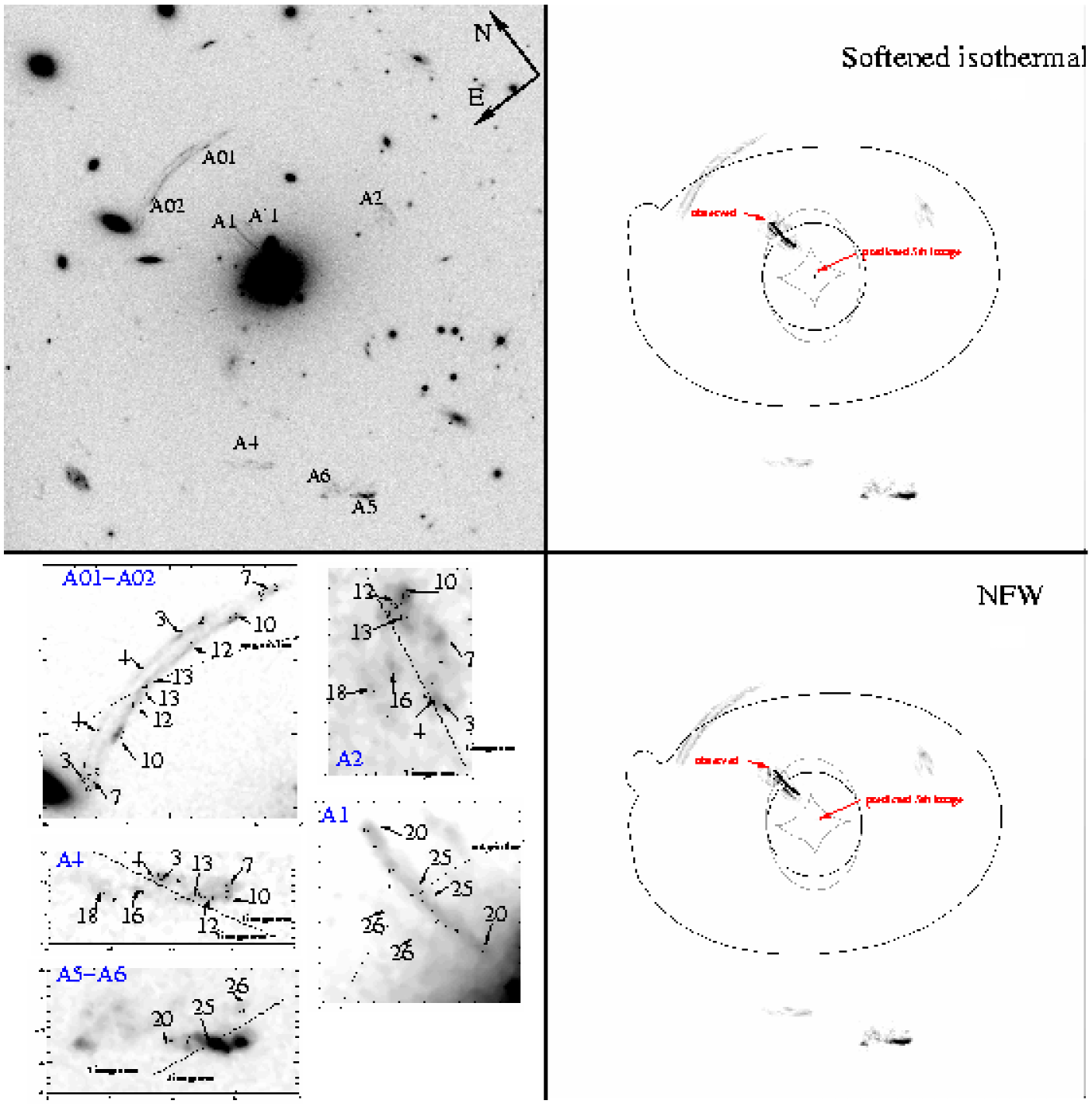
Figure 1: Upper left panel : overview of the lens configuration. The three arcs systems {A01,A02,A2,A4}, {A1,A5} and {A’1,A6}. The central cD galaxy. This F702 HST field is $56\times 56$ arcsec wide (i.e. $180\times 180\,\,h^{-1}\,{\rm kpc}$). Upper (resp. lower) right panel : reconstruction of arcs deduced from the single component best fit IS (resp. NFW) model (see 3.2). In these panels are reported the observed radial arc location. The small azimuthal offset is discussed in Sect. 4.2. The fifth demagnified image predicted by the models near the center is detailed in Fig 4. Lower left panel, detail of some dots used for the model fitting (see Table 5).

2.3 New insight on the light distribution

The HST data have been obtained from the Space Telescope archive. They consist in 10 WFPC2 images obtained with the F702W filter. The individual frames were stacked using the IRAF/STSDAS package, leading to a final exposure time of 22,000 sec. In addition, we used new data sets obtained during Summer 2001 with the VLT/FORS instrument in optical $UVI$ bands and with the VLT/ISAAC instrument in $J$ and $K$. The FORS and ISAAC data have been processed at the TERAPIX data center. Pre-calibrations, astrometric and photometric calibrations as well as image stacking were done using standard CCD image processing algorithms. We also used the $B$ and $R$ images kindly provided by S. Seitz that were obtained by the FORS team during the 1999 and 2000 periods. The exposure times of these data are shorter than our $UVI$ and $JK$ data, but they are still useful for the photometric redshift estimates.

Table 1: A brief summary of the VLT data. The first column summarizes the seeing of the final stacked images, the total exposure time is given in the second column. Also given the Magnitude Zero Points (Z.P.). The $B$ and $R$ images were obtained by the FORS team (provided by S. Seitz).

Filter	Seeing($\arcsec$)	Exp. time (sec)	Z.P (mag)
U	0.72	5280	30.856
B	1.2	2400	32.888
V	0.64	6900	33.978
R	0.58	300	32.501
I	0.69	12000	33.484
J	0.49	5880	27.643
K	0.50	6480	26.797

The MS2137.3-2353 optical data provide the azimuthal stellar light distribution and show that its geometry is elliptical. Its ellipticity increases with radius, starting from an almost circular shape at the center, and reaches quickly a constant value of 0.30 beyond the giant tangential arc location ($r\geq 15\arcsec$). The position angle is $PA\approx(71\pm 4)^{\circ}$ at $r=15\arcsec$ (see Fig 2). Assuming a fiducial mass-to-light ratio $\Upsilon_{I}=2$ and a I-band K-correction of 0.23, we evaluate the rest-frame I luminosity $L_{I}=1.9\times 10^{11}\,h^{-1}\,{\rm L}_{\odot}$.

The early ROSAT results of Gioia et al. (1990) and Ettori & Fabian (1999) and the recent Chandra observations of Wise & McNamara (2001) provide additional clues on the cluster halo. They confirm it appears as a well relaxed cluster. The X-isophotes are remarkably elliptical and do not show substructures. The orientation of gas is almost constant $PA_{X}=58^{\circ}\pm 7^{\circ}$, (see Fig 2). A new interesting observational feature is the global misalignment between the diffuse stellar component and the hot intra-cluster gas. It suggests that the stellar light distribution does not match exactly the DM distribution. This point is independently confirmed by strong lensing models and is discussed in Sect. 4.2.

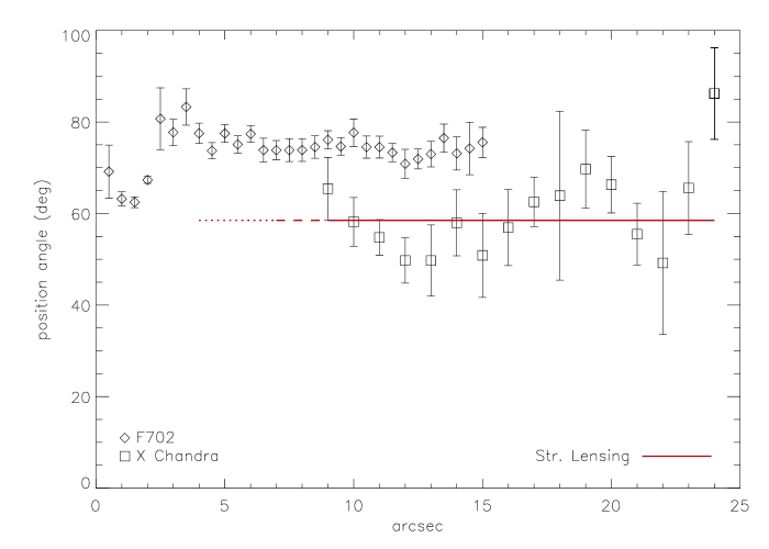
Figure 2: Orientation of the isophotal major axis as a function of radius. (squares: intra-cluster gas, diamonds: stars in the F702 band). The horizontal line represents the average orientation of the DM halo from modeling beyond $\sim 8\arcsec$. See Sect. 3.

The MS2137.3-2353 radial properties inferred from X-rays data reveal that the brightness profile presents a $r_{c}\sim 7\arcsec$ core radius and an asymptotic slope $\alpha\sim 1.17$, and an index $\beta\sim 0.56$. Ettori & Fabian (1999); Allen et al. (2002) modeled the X-ray emission and derived a gas mass fraction $f_{rmgas}\approx 0.10-0.15$ depending on the inferred cosmology. In both cases, this value is almost constant between 30 and $300\,h^{-1}\,{\rm kpc}$. Since the geometry of X-ray emission follows the overall potential and represents a small and constant mass fraction,we will not consider separately the gas and the dark matter in the lens modeling of MS2137.3-2353 in the following. Instead, we will simply reduce both components to an effective dark matter halo as the sum of the gas and true DM model. As a prospect, a good refinement would be the full introduction of this component, independantly of the DM halo. Moreover, a fully 3D deprojected modeling of both the X-ray emissivity and the strong lensing arcs system would certainly be the next requirement for future modelings.

2.4 VLT photometry & redshifts determination

The photometric redshifts of arcs have been measured with the hyperz software (Bolzonella et al, 2000; Pelló et al., 2001). The redshift $z_{\rm ph}$  is derived from a comparison between the spectral energy distribution of galaxies inferred from the $UBVRIJK$ photometry and a set of spectral templates of galaxies which are followed with look-back time according to the evolution models of Bruzual & Charlot (1993) (see Athreya et al., 2002, for details). The validation of hyperz is discussed in Bolzonella et al (2000) and has been already validated using spectroscopic redshifts on many galaxy samples. With the $UBVRIJK$ set of filters, it is possible to measure all redshifts of our selected galaxy sample lying in the range $0.0<z<3.5$. The expected redshift accuracy is between $\pm 0.05$ and $\pm 0.2$, depending on the magnitude of each arc, which is enough to scale the convergence of a lens model.

For each arc, the $UBVRI$ and $JK$ photometry was done as follows. We used SExtractor (Bertin & Arnouts, 1996) to estimate magnitudes in $2\arcsec$ apertures around a well defined barycenter for each part of the arcs. The $V$ frame is taken as the reference since arcs are significantly bluer than the cD light. We also tried to take the $U$ and $J$ ones to check the robustness of the method. As well, results are stable against variations of aperture.

Table 2: Photometric redshifts. Uncertainties take into account the scatter in the best fits with different choices for photometric measurements (aperture size, reference filter…). Note that HST data are not used for photometry.

Arc	A01	A02	A2	A4
$z_{\rm ph}$	$1.64\pm 0.15$	$1.6\pm 0.1$	$1.7\pm 0.2$	$1.58\pm 0.2$
Arc	A1	A5	A’1	A6
$z_{\rm ph}$	–	$1.60\pm 0.1$	–	$1.1\pm 0.3$

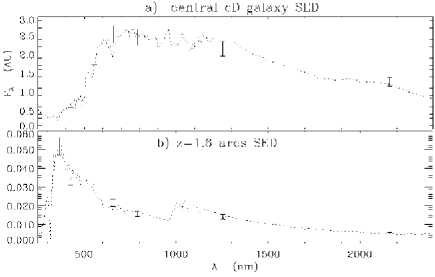
Figure 3: Spectral Energy Distributions resulting from photometric redshift analysis. a) Central cD galaxy at z=0.313 and b) arc A5 deduced to be at $z\simeq 1.6$. One can see that contrast between arcs and cD is 15 times higher in $U$ then in a redder filter like F702.

For the radial arcs A1 and A’1, photometry is strongly sensitive to the foreground cD diffuse stellar component. Furthermore, A1 and A’1 are overlapping, so no estimation of photometric redshifts are really stable for these objects. A better estimation of their redshift is provided by their counter-arcs which both are free from contamination. Results for all multiple images systems are summarized in table 2.
Taking the best determination, we conclude that $z_{s}=1.6\pm 0.1$ for the two sources responsible of the radial and tangential arc systems. The models detailed in Sect. 3.2.2 explain the need for a different redshift of the source responsible of A’1 and A6 and is consistent with the photometric redshift $z_{\rm s,A^{\prime}1-A6}\approx 1.1$. Hence, the critical density at the cluster redshift and with the adopted cosmology is:

$$\Sigma_{\rm crit}=3.73\times 10^{9}\,h\,{\rm M}_{\odot}{\rm kpc}^{-2}.$$

Sand et al. (2002) have recently reported a spectroscopic determination of the redshift of arcs which are both found to be at $z=1.501$ in remarkably good agreement with our color determination. From a gravitational lensing and mass estimate point of view, the difference between their spectroscopic redshift and our photometric prediction is un-significant. The geometric efficiency term $D_{ds}/D_{s}$ is slowly varying at this redshift. We nevertheless use their redshift estimation and the following value for the critical density:

$$\Sigma_{\rm crit}=3.78\times 10^{9}\,h\,{\rm M}_{\odot}{\rm kpc}^{-2}.$$

2.5 Detection of the fifth central image

Gravitational optics with a smooth potential and no central singularities predict strong magnification should produce an odd number of lensed images (Burke, 1981; Schneider et al., 1992). More generally, the location, the demagnification or even the lack of the central image are in principle clues on the properties of the innermost density profile of lenses.

In the case of MS2137.3-2353, we expect the large arc A0 to have a fifth demagnified counter-image. Unfortunately, any simple mass models of the lens configuration predicts the fifth image of this fold configuration should lie within one or two arc-seconds from the cluster center, that is inside the central cD light distribution. Its detection is therefore uncertain and depends on its surface brightness, its size and its color with respect to the cD light properties.

In order to check whether the fifth image associated to A0 is technically detectable, we made several lens models using different mass profiles which all successfully reproduce the tangential and radial arcs together with their corresponding counter-images. We predict its position $\@vec{r}_{5}$ and magnification from the softened IS and the NFW profiles of Sect. 3.2. They are respectively $\mu_{\rm IS}(\@vec{r}_{5})=0.2$ and $\mu_{\rm NFW}(\@vec{r}_{5})=0.1$. The signal-to-noise ratio per HST/F702 pixel yields :

$$\left(\frac{S}{N}\right)_{\rm F702}^{\rm pix}=\left(\frac{N_{5}}{1+N_{\rm cD}/N_{5}+N_{\rm sky}/N_{5}}\right)^{1/2}\simeq 0.7$$ (3)

where $N_{5}$, $N_{\rm cD}$ and $N_{\rm sky}$ are the number of photo-e^- from respectively the fifth image, the cD and the sky background close to $\@vec{r}_{5}$. Taking into account the size of the image, we can express the signal-to-noise in terms of flux, $\left(S/N\right)_{\rm F702}^{F}$, as a function of the magnification $\mu(\@vec{r}_{5})$ (assuming that the magnification $\mu(\@vec{r}_{\rm A2})$ does not much change with models).

$$\left(\frac{S}{N}\right)_{\rm F702}^{\rm F}\simeq 7\times\sqrt{\mu(\@vec{r}_{5})}.$$ (4)

The expected signal-to-noise ratio is $\approx$ 3 in the IS case and $\approx$ 2 for the NFW profile. So, in principle, the fifth image of the MS2137.3-2353 lensing configuration is detectable.

Using the counter-image A2 of area $A_{\rm A2}$ and flux $F_{\rm A2}$, we reconstructed the predicted fifth image satisfying :

$$\left\{\begin{array}[]{cc}F_{5}=\mu(\@vec{r}_{5})\times\mu(\@vec{r}_{\rm A2})^{-1}\times F_{\rm A2}\\ A_{5}=\mu(\@vec{r}_{5})\times\mu(\@vec{r}_{\rm A2})^{-1}\times A_{\rm A2}\end{array}\right.$$

and inserted it inside the cD galaxy at several positions close (but different) to the expected location $\@vec{r}_{5}$. We then determined the significance of several extraction-detection techniques on the Space Telescope image. A Mexican-hat compensated filter turned out to provide the best cD light subtraction and an optimal detection of the fifth image twins we put inside at different positions. In all cases it was detected exactly at the right position, whatever its location inside the cD and with the expected signal-to-noise.
Because we used a compensated filter which smoothes the signal, this later is not straightforward and we had to compare the amplitude of the flux contained in the extracted object to the variance of the background contained inside independent cells of similar size ranging along concentric annuli located at the radius where simulated fifth image twins are putted ($0.6\arcsec\lesssim r\lesssim 0.9\arcsec$). The averaged S/N found in annuli is 2.6, but it scatters between 1.3 and 3.5 depending on the local noise properties.

Table 3: Properties of the fifth images on real data (R.) and predicted from the best lens modeling (IS or NFW). The positions $(x,y)$ are given in arc-sec, with respect to the cD centroid. Position angles (P.A.) are given in degrees and $a/b$ is the axis ratio. The errors are found from the changes when varying some SExtractor parameters. Although both the position angles and the ellipticity of the IS and NFW are compatible with the data, there is a significant difference in positions. The offset $|\delta\@vec{x}|$ between the IS and the real position is only $0.16\arcsec$, whereas it is $0.36\arcsec$ for NFW, which is larger than uncertainties on observations (third column $|\delta\@vec{x}|\sim 0.05\arcsec$)

ID	$(x,y)$	$|\delta\@vec{x}|$	P.A.	$a/b$	S/N
R.	(0.64;0.70)	0.05	$28\pm 14$	$3.1\pm 1.3$	2.6
IS	(0.52;0.81)	0.16	15.	2.2	2.6
NFW	(0.33;0.52)	0.36	27.	2.2	2.1

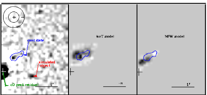
Figure 4: Visualization of residuals from subtraction of the cD brightness. Orientation is the same as in Fig 1. Left panel: HST filtering. One can see the real residual as well as a simulated object derived from the IS model shown on the right panel. Note the comparable signal-to-noise. Also plotted the Mexican-hat filter size with both positive ($r\leq 1.5\,{\rm px}$) and negative areas ($1.5\,{\rm px}\leq r\leq 3.5\,{\rm px}$) Also shown the noise-free reconstructed 5th image of the fold arc expected from IS (middle panel) and NFW (right panel) strong lensing best fit models centered on the cD. The position is consistent with the IS model. Note that the filtering algorithm reduces the high frequencies in the upper frame. Thus, shape measurements just provide rough estimates of ellipticities, but accurate orientations. Note also that the isophote plotted here, is illustrative and does not correspond to the any quantitative shape measurement.

The application of the extraction technique on the real data is straightforward. The brightest residual in the filtered frame shown in the right panel of Fig 4 is detected at the expected location when compared to models and is clearly the most obvious object underneath the cD. The object properties are listed in Table 3. They are remarkably similar to the IS and NFW fifth image predictions. Its coordinates are however closer to the IS fifth image than the NFW model. The signal-to-noise ratio of the candidate is $\simeq 2.5$, in very good agreement with our expectations. In the frame of Fig 1, the centroid position of the candidate is at

$$\@vec{r}_{5}=(0.64\arcsec;0.70\arcsec),\quad r_{5}=0.9\arcsec.$$ (5)

Despite its poorly resolved shape, the candidate exhibits an orientation $PA\simeq 28\pm 14^{\circ}$ and an axis ratio $a/b=3.1\pm 1.4$, in good agreement with the values predicted by both models (see Table 3). It is worth noticing that even the morphology of the fifth image shows similarities with the reconstructed images. In particular, it shows a bright extension inward and a smaller faint spot outward as if it would be dominated by two sub-clumps which are also visible on predictions of Fig. 4. In the following, when using the fifth image knowledge, we apply different weights on the detected features for the lens modeling. The brightest part of the fifth image is statistically significant and is associated to the dot labeled (10) on Fig. 1 and table 5. The mappings of the other labeled dots are not as significant in the fifth image. Thus, we apply a $\sim 9$ times smaller weight (i.e. 3 times larger errorbars). In other words, the fifth image is almost reduced to a point-like information without shape measurements.

3 The dark matter distribution in MS2137.3-2353

In this section, the properties of the dark matter distribution of MS2137.3-2353 are discussed in view of the most recent constraints we obtained from VLT data. We first revisit a single potential model using only strong lensing data but no fifth image. We then compare the projected mass profiles of the best NFW and IS models, extrapolated beyond the giant arcs positions, with the weak lensing analysis. Finally the fifth image is included in the strong lensing model which is used together with the weak lensing and the cD stellar halos to produce a comprehensive model of the different mass components.

3.1 Strong lensing optimization method

The optimization have been carried out with the lensmodel (Keeton, 2001b) inversion software. This alternative to the Mellier et al. (1993) or Kneib et al. (1993, 1996) algorithms allows us to check the efficiency and the accuracy of this software for arc modeling and to take advantage of its association tool for multiple point-images. This facility was initially developed by Keeton for multiple-QSOs but turns out to be well suited for HST images of extended lensed objects. The images association is performed by identifying conjugated substructures like bulges in extended images. Because of the surface brightness conservation, brightest areas in an image map into the brightest of the associated ones.

Our modeling started by identifying the brightest conjugate knots in each image. More precisely, when the identification of $N_{\rm knots}$ distinct features in images is completed (with respectively $N_{j=1\ldots N_{\rm knots}}$ multiplicity) one can write $N_{\rm knots}$ times the lens equation relating source and image positions and the lens potential $\phi$:

$$\@vec{\theta}_{S_{j}}=\left\{\begin{array}[]{l}\@vec{\theta}_{1}-\nabla\phi(\@vec{\theta}_{1})\\ \ldots\ldots\\ \@vec{\theta}_{N_{j}}-\nabla\phi(\@vec{\theta}_{N_{j}})\\ \end{array}\right.$$ (6)

This yields the following $\chi^{2}$ definition calculated in the image plane :

$$\chi^{2}_{\rm img}=\sum_{j=1}^{N_{\rm knots}}\sum_{i=1}^{N_{j}}\delta\@vec{x}_{ij}^{T}S^{-1}_{ij}\delta\@vec{x}_{ij},$$ (7)

with

$$2\sum_{j=1}^{N_{\rm knots}}(N_{j}-1)-N_{\rm par}$$ (8)

degrees of freedom, where $N_{\rm par}$ is the number of free parameters in the model. Here, $S^{-1}_{ij}$ is the error matrix for the position of knot $j$ in the image $i$ and $\delta\@vec{x}_{ij}=\@vec{x}_{{\rm obs},ij}-\@vec{x}_{{\rm mod},ij}$. Analogous $\chi^{2}$ minimization can be done in the source plane in order to speed up the convergence process. It is only an approximation of the previous one that does not directly handle observational errors in the image plane. However, it is much faster because it does not need to invert Eq. (6). Once the minimum location is roughly found, one can use the image plane $\chi^{2}_{\rm img}$ to determine the best parameter set with a better accuracy.

It is worth noting that the uncertainties in the conjugate points positioning done during the association process dominates the astrometric errors in the position of each knot. Typically, the systematic uncertainty is of order $0.1-0.2\arcsec$. The VLT color similarities were also used to confirm the associations. The mapping between extended images is given by the magnification matrix $a$ :

$$a^{-1}_{ij}(\@vec{\theta})=\delta_{ij}-\partial_{i}\partial_{j}\phi(\@vec{\theta}),$$ (9)

where $\delta_{ij}$ is the Kronecker symbol. Hence, other fainter conjugate dots become easier to identify once the local linear transformation between multiple images is known. The procedure “get constraints”-“fit a model” can be iterated to use progressively more and more informations.

In MS2137.3-2353, we kept 13 unambiguous quintuple conjugated dots in the tangential arc A01. Each one is associated to four different dots in A02, A2, A4 and the fifth image. We selected also 6 dots in the parts of A2 and A4 that are only triply imaged. Likewise, A1 is decomposed in two symmetric merging images and is also associated with the Eastern part of A5 (6 triple conjugated dots). Fig. 1 and table 5 summarize the associations we selected.

The various models are actually over-constrained. The 6 free parameters are detailed in the following section. Following Eq. (8), the number of constraints is

$$N=2\times\{13(5-2)+6(3-2)+7(3-1)\}=118.$$ (10)

The first term corresponds to the regions of the tangential system which are imaged five times, whereas the second term refers to regions imaged three times. The third term correspond to the radial system which is imaged three times. Nevertheless, only 25 of these 118 constraints appear significant to represent the first and second shape moments of arcs, the rest is for higher order moments and have less weight in the modeling.
A galaxy at the eastern part of A02 should weakly perturb its location and shape. This galaxy was introduced in previous models but turns out to have negligible consequences. Indeed, only upper limits on its mass ($\sigma_{v}\lesssim 150\,km/s$) arise when modeling. Its introduction appears marginally relevant for the study and is ignored hereafter although its effect is shown on Fig 1.

3.2 Strong lensing models without the fifth image

3.2.1 Dark matter density profiles

We model the dark matter halo with two different density profiles. In order to focus on the main differences between isothermal and NFW profiles, we keep the models as simple as possible and do not include peculiar features, like cluster galaxy perturbations. The center of potential is allowed to move slightly within 2 arc-sec around the cD of the cD galaxy. No prior assumptions are made about the ellipticity and the orientation of the dark matter halo relative to the light nor to the X-rays isophotes.

The first profile is an elliptical isothermal distribution with core radius of the form,

$$\rho(r)=\frac{\rho_{c}}{1+(r/r_{c})^{2}}\quad{\rm\leavevmode\nobreak\ in\leavevmode\nobreak\ spherical\leavevmode\nobreak\ approx.}$$ (11)

which is projected in,

$$\kappa(r,\theta)=\frac{b}{\sqrt{\xi^{2}+r_{c}^{2}}},\quad\xi=r\sqrt{1-\epsilon\cos(2(\theta-\theta_{0}))}.$$ (12)

The core radius $r_{c}$, scale parameter $b=r_{c}+\sqrt{R_{e}^{2}+r_{c}^{2}}$, ellipticity $\epsilon$ and position angle $\theta_{0}$ are free parameters. $R_{e}$ is the Einstein radius and $b$ is related to the cluster velocity dispersion by

$$b=\left(\frac{\sigma_{v}}{186.5\,km.s^{-1}}\right)^{2}\frac{D_{ds}}{D_{s}}\quad{\rm arc-sec.}$$ (13)

The second profile is an elliptical NFW mass distribution. The 3D profile has the form

$$\rho(r)=\frac{\rho_{c}\delta_{c}}{(r/r_{s})(1+r/r_{s})^{2}}\;\;\;\;\;\text{in spherical approx.}$$ (14)

where $r_{s}$ is a scale radius, $\rho_{c}$ is the critical density of the universe at the redshift of the lens, and $\delta_{c}$ a concentration parameter related to the ratio $c=r_{\rm 200}/r_{s}$ by

$$\delta_{c}=\frac{200}{3}\frac{c^{3}}{\ln(1+c)-c/(1+c)}.$$ (15)

The convergence $\kappa$ writes

$$\kappa(r,\theta)=2\kappa_{s}\frac{1-F(x)}{x^{2}-1}\;\;\text{with\ \ }x=\xi/r_{s}\;,$$ (16)

where $\xi$ has the same meaning than before, $\kappa_{s}=\rho_{c}\delta_{c}r_{s}/\Sigma_{\rm crit}$ and

$$F(x)=\left\{\begin{array}[]{cl}\frac{1}{\sqrt{x^{2}-1}}\tan^{-1}\sqrt{x^{2}-1}&\text{, for }x>1\\ \frac{1}{\sqrt{1-x^{2}}}\tanh^{-1}\sqrt{1-x^{2}}&\text{, for }x<1\\ 1&\text{, for }x=1\end{array}\right.$$ (17)

3.2.2 Single halo best models

The inversion leads to two models that fit the strong lensing observations equally well. They reproduce the multiply-imaged lens configuration of both radial and tangential arcs. The NFW best fit model leads to a $\chi_{\rm NFW}^{2}=2.42$ per degree of freedom and $\chi_{\rm IS}^{2}=3.0$ for the isothermal profile. The final model parameters and errors bars are summarized in table 4. The centering of the dark matter halo relative to the cD galaxy is discussed in Sect. 3.4.1.

Table 4: Single halo models. The Einstein radius is the same in the best models for strong lensing : $R_{E}\simeq 50\,h^{-1}\,{\rm kpc}$. For our two strong lensing models, the total mass inside this radius is $M(r<R_{E})=(2.8\pm 0.1)\times 10^{13}\,h^{-1}{\rm M}_{\odot}$. Errors due to uncertainties in arcs redshift are omitted. Also reported previous works results for comparison. Me93 refers to (Mellier et al., 1993), Ha97 to (Hammer et al., 1997), Mi95 to (Miralda-Escudé, 1995) EF99 to (Ettori & Fabian, 1999) and Al02 to (Allen et al., 2002). When known, the authors’ values are recomputed in our adopted cosmology and with the 1.6 sources redshifts. For both papers, the center of potential location is assumed to match the center of cD or is not reported. Me93 core radii have been scaled in order to take into account the departs between their profile and an exact softened isothermal sphere. As well, Ha97 find a slope $\beta\approx 0.85$ instead we have only considered models with $\beta=1$ (see Eq. (2)). Al02 uses a NFW profile and only gives the scale radius value but we report on the same line our own measured values for ellipticity and position angle from Chandra X-ray brightness. The third column $r_{c}\backslash r_{s}$ corresponds either to the scale radius either to the core radius. Here, we convert all the position angles in a common definition, which is clockwise from North to East. The original paper do not report angles in the same frame but we made the correction except for Ha97 for which we do not know what is the reference. But in any case, the position angle is so constrained that these authors must have found a similar orientation as the other ones. Our definition is more valuable and self-consistent between Chandra, ROSAT, VLT and HST data. Models labels with a S refer to purely strong lensing modeling whereas a W stands for purely weak lensing fits. The last row (cD+DM) concerns the last family of profiles with a cD and dark matter halo components and which is simultaneously constrained by strong+weak lensing. In the first column, we report the permitted inner slope for generalized NFW profiles (see Sect. 3.4.3).

model	$\sigma_{v}$	$r_{c}\backslash r_{s}$	$\kappa_{s}$	$r_{\rm 200}$	c	$M_{\rm 200}$	$\epsilon$	$PA$	$x_{c}$	$y_{c}$
	(km/s)	$(\,h^{-1}\,{\rm kpc})$		$(\,h^{-1}\,{\rm kpc})$		$(10^{14}\,h^{-1}\,{\rm M}_{\odot})$		deg	arcsec	arcsec
S-NFW	-	$90^{+35}_{-25}$	$0.6^{+0.5}_{-0.3}$	$920^{+180}_{-80}$	$12.5^{+5}_{-6}$	$\sim 5.5$	$0.24^{+0.04}_{-0.07}$	$58\pm 1$	$0.1\pm 0.4$	$0.2\pm 0.4$
W-NFW	-	$67^{+300}_{-24}$	$0.74_{-0.5}^{+1.6}$	$890^{+160}_{-130}$	$12_{-8}^{+12}$	-	-	-	-
S-isoT	$1022^{+40}_{-30}$	$10.4\pm 1.8$	-	$\sim 1000$	-	$\sim 11.$	$0.25\pm 0.05$	$59\pm 1$	$0.2\pm 0.4$	$0.2\pm 0.4$
W-isoT	$900\pm 150$	$<45$	-	-	-	-	-	-	-
Me93	$\sim 1000$	$4.5-7$	-	-	-	-	$0.15-0.33$	$51-66$	-	-
Mi95	$\sim 1200$	$\sim 10$	-	-	-	-	$\sim 0.22$	$\sim 58$	-	-
Ha97	$\sim 1100$	$5-10$	-	-	-	-	$0.18-0.23$	$?47.5\pm 5?$	-	-
EF99	$\sim 930$	$\sim 90$	-	$r_{500}\sim 540$	-	-	-	-	-	-
Al02	-	$107-120$	-	-	-	-	$\sim 0.20$	$58\pm 7$	-	-
cD+DM	$0.8<\alpha<1.1$	$\sim 85$	$\sim 0.6$	-	-	-	$0.22\pm 0.06$	$58\pm 2$	0!	0!

The associated counter-image of the radial arc A1 (bright and thin structure) corresponds only to a small part of A5 that is triply imaged. Besides, the diffuse component A’1 can be associated to A6 only if the corresponding source is at a lower redshift than arc A1-A5. This corroborates photometric redshifts results and was previously mentioned by Hammer et al. Here, we find the source redshift $z_{\rm S(A6-A^{\prime}1)}$ to be $1.1-1.3$.

The velocity dispersion derived for the IS model is consistent with results of Mellier et al. (1993). The core radius proposed by these authors is higher because of its different definition. They used a pseudo-isothermal projected gravitational potential; instead, we directly model the cluster projected density profile. Nevertheless, to ensure the same Einstein radius with the same central velocity dispersion between their model and ours, the core radius they reported must be twice the one we found. Thus, core radii are consistent.

3.3 Mass profile of MS2137.3-2353 from weak lensing analysis:

Although the error bars are large, the concentration parameter found for the best NFW model is about twice the expectations from numerical simulations and from the current measurements done in other clusters, even those with strong lensing features (See e.g. Hoekstra et al., 2002). Since clusters are believed to be triaxial, it may happen that the major axis lies along the line of sight, increasing atificially its concentration by projection effects (See e.g. Jing & Suto, 2002). However, it is likely that our model also mix together the contributions to the effective concentration of the cluster and of the central cD potentials. This possibility can be tested by comparing the strong lensing model with the weak lensing anlysis that only probes the radial mass profile at larger scale, where the cD contribution is negligible. On large scales, we used the VLT images to build a weak lensing catalog of background galaxies covering a $6.4^{\prime}\times 6.4^{\prime}$ field of view. At the cluster redshift, this corresponds to a physical radius of $700\,h^{-1}\,{\rm kpc}$. The detailed description of the catalog analysis, namely PSF anisotropy corrections and detailed galaxy weighting scheme and selection, is beyond the scope of this work. The method we used can be found in (Athreya et al., 2002). Here, we only compare the result of the strong lensing mass profile and the fit of the azimuthally averaged shear on scales $100\,\,h^{-1}\,{\rm kpc}\lesssim r\lesssim 1\,{\rm Mpc}$.
The shear profile is determined by using a maximum-likelihood analysis, based on a $\chi^{2}$ minimization:

$$\chi^{2}=\sum_{i=1}^{N}\frac{|e_{i}-g(\@vec{r}_{i},z_{i})|^{2}}{\sigma_{e,i}^{2}},$$ (18)

where $e_{i}$ is the complex image ellipticity, $g$ the complex reduced shear, $z_{i}$ the photo-$z$ and $\sigma_{e,i}$ the dispersion coming from both the intrinsic unknown source ellipticity and the observational uncertainties (See e.g. Schneider et al, 2000). In addition, we also measured the $\zeta$-statistic and $\zeta_{c}$-statistic densitometry:

$$\zeta(r;r_{\rm max}) = \bar{\kappa}(r^{\prime}<r)-\bar{\kappa}(r<r^{\prime}<r_{\rm max})$$ (19)

$$= \frac{2}{1-(r_{\rm max}/r)^{2}}\int_{r}^{r_{\rm max}}\left<\gamma_{t}(r)\right>{\rm d}\ln r,$$

$$\zeta_{c}(r;r_{2},r_{max}) = \bar{\kappa}(r^{\prime}<r)-\bar{\kappa}(r_{2}<r^{\prime}<r_{\rm max})$$ (20)

$$= \left[1-(r/r_{\rm max})^{2}\right]\zeta(r;r_{\rm max})+$$

$$\frac{1-(r_{2}/r_{\rm max})^{2}}{(r_{\rm max}/r_{2})^{2}-1}\zeta(r_{2};r_{\rm max})$$

where $\left<\gamma_{t}(r)\right>$ is the averaged tangential ellipticity inside an annulus ($\pi r^{2}\Sigma_{\rm crit}\bar{\kappa}(r)$ is the mass enclosed within the radius $r$). In contrast with the $\zeta$ statistics, $\zeta_{c}$ can be directly compared with $\bar{\kappa}$ since they only differ by a constant value that does not change with radius (Clowe et al., 2000). We used $r_{2}=517\,h^{-1}\,{\rm kpc}$ and $r_{\rm max}=744\,h^{-1}\,{\rm kpc}$.
The scaling factor for the mass has been derived from the $UBVRIJK$ photometric redshifts of sources. Background galaxies have been selected in the magnitude range $I<24$ and cluster galaxies have been rejected using a photo-$z$ selection. Moreover, we considered background galaxies with $z_{\rm ph}$$\,>0.4$ for which the lensing signal is significant. The limiting magnitude was chosen in order to compromise between the depth, which defines the galaxy number density, and the need for a good estimate of the source redshift distribution. Since our source population is similar to Van Waerbeke et al. (2002), we checked our redshift histogram has the same shape as their sample. Both samples turned out to be similar, so we finally used their parameterized redshift distribution, because it is based on a larger sample than ours. With this requirement, the weak lensing signal directly makes a test on the reliability of strong lensing models extrapolations beyond the Einstein radius.

Fig. 5 shows the radial mass profile of the best IS and NFW models. The projected mass density has been averaged inside circular annuli. As expected, the two best fits are quite similar between the two critical radii. Discrepancies only appear in the innermost and outermost regions. However, the shear profile derived from the VLT data fails to disentangle the models built from strong lensing. Both are consistent with the signal down to the virial radius $r_{\rm 200}\approx 1\,h^{-1}\,{\rm Mpc}$. Table 4 lists the values of the best fit parameter set for the weak lensing analysis. It is in good agreement with the inner strong lensing models, though the total encircled mass is smaller. The constraints on the concentration parameter are weak and a broad range of values are permitted. However, a low value similar as expectations for clusters is still marginal and surprisingly the weak lensing analysis also converges toward a rather larger concentration. This discrepancy with cluster expectation values, even when using together weak and strong lensing constraints, shows that the global properties of the potential well are hard to reconcile with a simple NFW mass profile. However, if the contribution of the cD stellar mass profile strongly modifies the innermost mass distribution of the cluster and significantly contaminates the concentration parameter inward, our statement based on strong and weak lensing models might be wrong. We therefore single out the cD potential and add its contribution to the model and we included the fifth image parameters in order to probe the very center where the cD mass profile might play an important role.

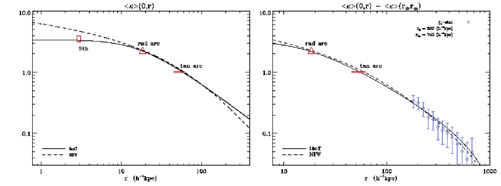
Figure 5: Projected mean surface density. Solid: NFW best fit, dashed: IS. Notice how models match near the arcs locations. Between 2.5 and 28 arc-sec, the mean convergences $\bar{\kappa}=<\kappa>(0,r)$ differ from each other by less than 3 percents. Faint discrepancies appear in the outer regions through weak lensing signal and at the very center. Constraints due to the fifth image candidate are detailed in Sect. 3.4.3. The weak lensing data are deduced from the $\zeta_{c}$-statistic.

3.4 The cD+DM mass profiles constrained with the fifth image.

We now consider a two-component mass profile : an inner stellar component attached to the cD galaxy and a cluster dark matter halo. The fifth central image will contribute to constrain the innermost lens model, whereas the external arcs and the weak lensing profile should constrain most of the outer cluster halo.

3.4.1 Centering the lens with the fifth image

Before introducing the stellar component, let us check the influence of the fifth image knowledge on the centering of a single DM potential. Fig. 6a shows the permitted area for the DM potential center relative to the cD. The contours on the top are the expectations for the IS and NFW models, if the fifth image is not taken into account. The offset with respect to the cD centroid is $0.22\arcsec$ West, but the contour ellipses are of size $1.1\arcsec\times 1.6\arcsec$. Nevertheless, the assumption that the center of cD galaxy coincides with the cluster center is consistent with the data.

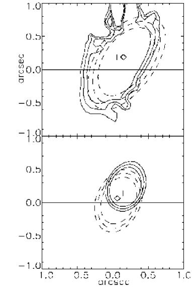
Figure 6: Permitted potential center region ($\Delta\chi^{2}/N=1,2,3$) relative to the cD center (0,0) coordinates. Solid (resp. dashed) contours refer to the NFW (resp. IS) model. The upper panel displays contours without the fifth image location knowledge and the lower using the 5th image candidate discussed in Sect. 2.5 as an additional constraint. The crosses (resp. diamonds) correspond to the $\chi^{2}$ minimum location for the NFW (resp. isothermal) modeling. Note the great enhancement induced and the significant shift in the NFW case compared to the upper panel. The deflection angle is merely too small to be consistent with the fifth image.

When the fifth image is added (mainly its brightest knot), the contours shrink by a factor of 2 in size, as shown in Fig 6b, but still keep the central cD position inside, with a small offset with respect to the cD light centroid of $0.16\arcsec$ West for the IS model, and $0.18\arcsec$ West for the NFW profile. The box sizes of permitted positions are much smaller ellipses of about $0.6\arcsec\times 0.9\arcsec$. Since these error boxes are about the size of the uncertainties of the cD centroid position (see Table 3), in the following we will then assume the cD is centered on the cluster center. It is worth noticing that even with the significant reduction of error bars provided by the fifth image, the residual uncertainty on the centroid position of the lens may in principle permit to both IS and NFW to fit the lensing data if we do not assume the cD center is not exactly on the cluster center.

3.4.2 Modeling together the stellar and DM mass profiles

The properties of the lens configuration (including the fifth image) provide enough constraints to attempt a modeling which will probe clear differences between observations and IS/NFW predictions. The deflection and the magnification of the NFW model are smaller than for an IS one. We expect the fifth image to show a difference of $0.2\arcsec$ in position and 0.75 in magnitude. The observations and IS/NFW predictions reported in table 3 and Fig. 4 already show a trend which supports a flat-core model against a cuspy NFW profile.
The following analysis uses together the fifth image properties, the weak lensing data and the giant arcs in order to constrain the shape of the innermost mass profile. We also add the cD stellar contribution to the overall mass because it is no longer negligible at the very center. Note that the generalized NFW models expressed in Eq. (1) has a free parameter $\alpha$. Its projection is reported in Eq. (27). In more details:

• The fifth image central coordinates are introduced because of their constraints on the central lens modeling. In fact, the brightest knot in the large arc A0 is required to correspond to the brightest detected spot at the center $r_{5}\approx 0.9$.

• The center of the cD is precisely the center of the potential well.

• The dark matter halo is modeled by an elliptical mass distribution: a softened IS profile or a generalized-NFW profile, as expressed in Eq. (27). Hence, the IS profile has 4 free parameters, namely $r_{c}$, $\sigma_{v}$, $\epsilon$, $PA$ whereas the generalized-NFW models has 5 : $\alpha$, $r_{s}$, $\kappa_{s}$, $\epsilon$, and $PA$.

• We model the stellar component with an Hernquist profile ($\rho(x)=x^{-1}(1+x)^{-3}$) of the projected form :

  $$\begin{split}\kappa_{*}(r)&=\frac{\kappa_{s,*}}{(y^{2}-1)^{2}}\left[-3+(2+y^{2})F(y)\right]\\ \bar{\kappa}_{*}(r)&=2\kappa_{s,*}\frac{1-F(y)}{y^{2}-1}\end{split}$$ (21)

  with $F$ defined in Eq. (17), $y=r/r_{g}$ and $r_{g}\approx 7.2\,h^{-1}\,{\rm kpc}$ a scale radius. $\kappa_{s,*}$ is related to the I band luminosity through the relation:

  $$\kappa_{s,*}=\frac{L_{I}}{2\pi s^{2}\Sigma_{crit}}\left(\frac{M}{L}\right)_{I}=0.11\Upsilon,$$

  where $\Upsilon\equiv M/L_{I}$. The stellar component is elliptical and has the central ellipticity $\epsilon_{*}=0.15$ and orientation $PA_{*}=69^{\circ}$ deduced from the light distribution in the I band. The cD stellar mass-to-light ratio $\Upsilon$ is the last new free parameter of the model.

• The weak lensing $\chi^{2}$ term (Eq. 18) is directly added to the purely strong lensing $\chi^{2}$ defined in Eq. (7).

3.4.3 The inner slope of the DM halo

The constraints provided by the fifth image can roughly be illustrated as follows. If $r_{5}\approx 0.9$ corresponds to a source position $u\approx 1.85\arcsec$ deduced from the single component outer arcs. The lens equation reads: $u=r_{5}\;|1-\bar{\kappa}(r_{5})|$ with the bending angle $\bar{\kappa}(r)=\tfrac{1}{r}\tfrac{\,{\rm d}\varphi}{\,{\rm d}r}$. Hence, the averaged convergence within the fifth image candidate radius which is plotted on Fig 5 is

$$2.9\lesssim\bar{\kappa}(<r_{5})\lesssim 3.7.$$

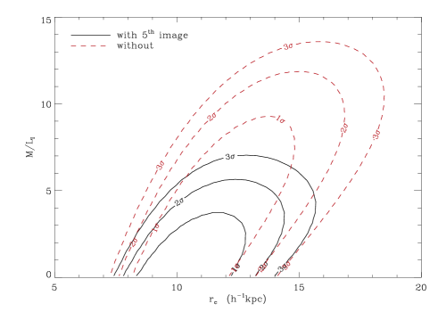
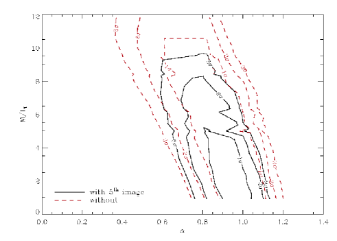
Figure 7: Two components $\chi^{2}$ contours. Upper panel : constraints on the couple $r_{c}-M/L_{I}$ for the IS model. Note the small modifications due to the introduction of the stellar component. Lower panel : constraints on the couple $\alpha-M/L_{I}$ for the pseudo-NFW family profiles. One can see an overlay of the same confidence regions when the fifth image position is known (solid) and when it is not (dashed). The inner slope $\alpha$ ranges between 0.8 and 1.1 for a reasonable mass of stars ($\Upsilon_{I}\leq 5$). The lower panel rejects very shallow profiles ($\alpha\leq 0.6$) whereas one can see on the upper one that flat cores provide good fits.

It is now possible to test the overall permitted central contribution by mapping the global $\chi^{2}$ in the $r_{c}-M/L_{I}$ or $\alpha-M/L_{I}$ spaces, after marginalization over the other parameters. For a reasonable mass-to-light ratio $\approx 2-3$, one can see on Fig 7 that :

• Both IS and generalized-NFW models rule out $M/L_{I}$ of the cD stellar component larger than 9 at a 3-$\sigma$ confidence level. Its value preferentially ranges within 1 to 5.

• The softened IS profile still provides the best model. It is also consistent with the strong lensing data with few variations of parameters compared to the single component modeling. The introduction of the stellar component does not introduce large variations in the best fit parameters set compared to the single dark halo modeling.

• The cuspy models have a narrow permitted range of slope which is centered around $\alpha=1$ of the NFW model. Note that while the position of the fifth image provides interesting boundaries on the cluster center position, it does not provide constraints on the slope $\alpha$. Including the fifth image only reduced the $\alpha$ upper limit by 10% and does not changes its lower bound. For reasonable values of $M/L_{I}$, we find $0.8\leq\alpha\leq 1.1$ (2-$\sigma$). This range excludes very low values of $\alpha$ and seems to contradict the fact that IS with flat core better fit the data than generalized-NFW models over the whole $1\,h^{-1}\,{\rm kpc}<r<600\,h^{-1}\,{\rm kpc}$ range, even for a large amount of stellar mass.

4 Discussion

4.1 The radial mass profile of MS2137.3-2353

The exceptional data set allowed us to constrain the density profile over three orders of radius ranging from 2 to 700 $\,h^{-1}\,{\rm kpc}$. Despite the fact that weak lensing data do not cover a wide enough range in order to reveal its full efficiency, we performed a self consistent modeling of the critical strong and sub-critical weak parts of the lensing cluster MS2137.3-2353. At the other side, it is worth noticing that the improvement provided by the fifth image is still under-exploited because of the poor resolution of its shape. The location of its brightest spot only provides constraints on the center position of the lens and on the overall enclosed mass (by the way, revealing a degeneracy between $\Upsilon$ and $\alpha$). A good knowledge of the magnification and shear would be able to break this degeneracy by constraining second order moments of the fifth image probing both convergence and shear inside 1 arc-sec radius.

Nevertheless, the new constraints provide three levels of information concerning the MS2137.3-2353 radial mass profile.

• The simple use of the radial and tangential arcs systems without the fifth image neither the outer shear data cannot disentangle between NFW-like and isothermal profiles. A large family of cuspy and flat models are consistent with these data. (See Figs. 8 and 9 and appendix B)

• The combined weak lensing and arcs (i) data tell us that either isothermal profiles either NFW-like profile with $0.8\lesssim\alpha\lesssim 1.1$ are permitted.

• Actually, the fifth image knowledge favors flat cores ($\chi^{2}_{IS}\sim 3.8$) but puts strong limits of the couple $\alpha-\Upsilon$ for NFW-like models ($\chi^{2}_{\alpha\sim 1}\sim 5.1$).

All together, the new constraints are in good agreement with isothermal model with flat core and rule out generalized-NFW models with slopes as steep as those proposed by (Moore et al., 1998; Ghigna et al., 2000). The slope range found for the generalized-NFW profiles can be easily explained and correspond to expectations. The calculations detailed in appendix B (Figs. 8 and 9) show how the knowledge of the lensing configuration, as derived from giant arcs and the shear field, bounds the free parameters for cuspy-NFW profiles. The knowledge of the critical lines radii, the weak lensing at intermediate scales as well as the length of the radial arc are introduced in order to fix semi-analytically $r_{s}$, $\alpha$ and $k_{s}$.

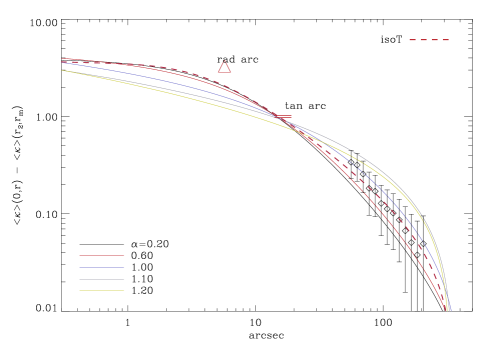
Figure 8: Plot of various $\zeta_{c}$ curves taken along the relation plotted in blue (light gray) on Fig 9 that give the observed critical lines. Also plotted the observed $\zeta_{c}(r)$ deduced from weak lensing. Only a small scatter around $\alpha=1$ is allowed. We also report the best fit isothermal profile (dashed).

A lower curvature for NFW-like profiles can explain the apparent paradox discussed at the end of Sect. 3.4.3. Flat softened isothermal profiles are favored whereas low values of $\alpha$ are ruled-out. This trend was reported by Miralda-Escudé (1995) when he tried to fit the dark matter halo with a density profile of the form

$$\rho(x)\propto x^{-1}(1+x)^{-3/2}\quad{\rm or\ \ }\rho(x)\propto x^{-1}(1+x)^{-1}.$$

Hence, a simple smooth modification from the inner slope $\alpha\ll 1$ to an asymptotic $\rho\propto r^{-3}$ outward cannot match the whole lensing data. Sharper changes must occur at a small radius which behaves as an effective core radius, leading to a high curvature close to the radial arc. The scale radii derived from the marginalization of Fig 7 are very small and still scatter around the $r_{s}\approx 90\,h^{-1}\,{\rm kpc}$ value obtained from the single component NFW. The sensitivity of models to radial curvature is clearly visible on Fig 8.

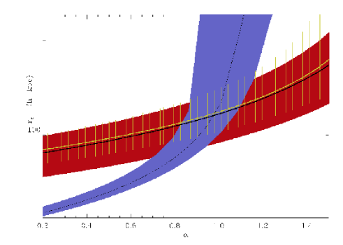
Figure 9: Relations in the parameter space $\alpha-r_{s}$ deduced from the critical lines Eq. (25a) and Eq. (25b) (blue or light gray region), from the $\zeta-$statistic and Eq. (25a) (red or dark gray) and from the radial arc length relative to its counter-image (dashed yellow area). Errors take into account variations of ellipticity, of the mass-to-light ratio and observational uncertainties. The resulting permitted region is well consistent with what is found from the modeling. One can see that $0.7\lesssim\alpha\lesssim 1.1$. In other words, the halo density profile must be much shallower than the value 1.5 suggested by recent numerical simulations (Moore et al., 1998; Ghigna et al., 2000). The permitted range for $r_{s}$ is restricted to small scale radii $r_{s}\sim 100\,h^{-1}\,{\rm kpc}$.

The whole best fit generalized-NFW profiles show a high concentration for the dark matter halo. This trend is confirmed by weak lensing up to $700\,h^{-1}\,{\rm kpc}$, in contrast with other weak lensing cluster analyses which find smaller concentration than ours, but more consistent with numerical CDM simulations. The role of stars does not change this conclusion. So, if generalized-NFW models are acceptable, it is important to confirm that in the case of MS2137.3-2353 they imply the concentration to be stronger than numerical predictions. It is therefore important to confirm these results by using a different method. Recently, Sand et al. (2002) have reported comparable slope constraints using the velocity dispersion of stars at the center of the cD and the positions of critical lines. Conversely, any lensing model should be consistent with the information on the kinetic of stars they measured, so it is necessary to compare our predictions with their data. Nonetheless we plan to show elsewhere (Gavazzi et al., in preparation) that the velocity dispersion usually measured from the FWHM of absorption lines in the galaxy spectrum no longer hold if the distribution function of stars is far from a Maxwellian as mentioned in Miralda-Escudé (1995).

Finally, we checked that the introduction of galaxy halo perturbations under the form of massive haloes attached to the surrounding cluster galaxies does not change our conclusions. Such perturbations have poor consequences for the weak lensing results but are likely affect slightly the fifth image location. We show in appendix C that a significant modification of the fifth image due to galaxy halo perturbations implies to put a huge mass on each galaxy. Such an amount of mass would destroy the quality of the arcs fit.

4.2 Effects of non constant ellipticity and isodensity twist on the radial arc

At the tangential arc radius ($r\sim 50\,h^{-1}\,{\rm kpc}$) we measure a robust offset angle $\Delta\theta=13^{\circ}\pm 4^{\circ}$ between the diffuse stellar component and the DM potential orientation. This result is confirmed by the Chandra X-rays isophotes contours as shown on Fig 2. Previous strong lensing modelings in the presence of important cD galaxies never clearly established such a behavior because the uncertainties of the models obtained with tangential arcs only were too loose for the isopotential orientation.
However, for the nearby elliptical galaxy NGC720 Buote et al (2002) and Romanowsky & Kochanek (1998) studied such a misalignment between the light distribution and the surrounding dark halo revealed by X-ray emissivity. RK showed that the stellar misalignment can be explained by a projection effect of triaxial distributions with aligned main axis but different axis ratios.

Moreover all the best fit modelings show a tiny but robust remaining azimuthal offset ($\lesssim 0.3\arcsec$) between the modeled radial arcs (A1 and A’1) and the position actually observed on the HST image (highlighted on reconstructions of Fig 1).
We verified that it is not due to a bad estimation of the source position since any small source displacement produces a large mismatch between the counter-arc A5 and the model. This pure azimuthal offset led us to investigate the possible effect of a variation of the ellipticity and position angle of the projected potential close to the radial arc radius. Such a trend is also favored by an increase of ellipticity on the X-ray isophotes with radius.

If we had implemented the availability of using models with a variation of orientation and ellipticity with radius in the inversion software, we would have found that the orientation of the potential major axis tends to the orientation of stars (see Fig 2) when looking further in. At the same time the potential becomes rounder. We roughly checked this behavior by modeling the lens configuration with two distinct (and discontinuous) concentric areas (inside and above 8 arc-sec). The rays coming from the source plane and giving rise to the outer arcs A0, A2, A4, A5 do not suffer any inner variation of the potential symmetry (provided that the overall mass inclosed in the Einstein radius remains the same). Hence the previous modelings remain valid for the outer parts whereas the inner can be twisted and made rounder in order to alleviate the offset problem. A small twist $\Delta\,PA\simeq 8^{\circ}$ in the direction of stars gone with a smaller ellipticity ($\epsilon\simeq 0.2$) turns out to suppress efficiently the azimuthal offset near the center without affecting the external arcs. This analysis is not exhaustive in the sense that maybe different explanations can be found but its main virtue is to show that high spatial resolution like HST imaging of numerous multiple arcs makes a lens modeling so binding that it becomes possible to extract much more information than the simple fit of elliptical models. In addition with the hot ICM properties (see e.g.  Romanowsky & Kochanek, 1998), we could certainly start more detailed studies of potential with twist effects and eventually start to probe the triaxiality of dark matter halos if we can observe a large number of multiple arc systems in clusters.
These results strengthens the argument of Miralda-Escudé (2002) upon which the ellipticity of DM halos makes inconsistent the hypothesis of self-interacting dark matter.

5 Conclusion

By using strong and weak lensing analysis of HST and new VLT data of MS2137.3-2353 we found important new features on the lensing configuration:

The photometric redshifts or the radial and the tangential arcs are both at $1.6\pm 0.1$ in excellent agreement with the recent spectroscopic observations of Sand et al..
The extraction of the cD diffuse stellar light has permitted to detect only one single object which turns out to be at the expected position of the fifth image. Furthermore, its orientation, its ellipticity, its signal-to-noise ratio and its morphology correspond to those expected by the lens modeling. Unfortunately, the poor determination of its shape properties hampers the use of its geometry as a local estimate of the magnification matrix toward the center.
Using the fifth image together with the weak lensing analysis of VLT data, we then improved significantly the lens modeling. The radial mass profile can then be probed over three orders in distance. This additional constraint seems to favor isothermal profiles with flat core or generalized-NFW profiles with $0.8\leq\alpha\leq 1.2$ without introducing the fifth image knowledge. When this constraint is added together with the prior motivated that cD center and cluster halo center are the same, we favor flat core softened isothermal spheres. The position of the fifth image is in better agreement with an isothermal model than an NFW mass profile. In addition, it is worth noticing that the kinetics of stars should be analyzed in details, considering a precise distribution function that may depart from the commonly assumed Maxwellian.

We point out a misalignment between the diffuse stellar component major axis and both the lens potential and the X-ray isophotes. We argue it is produced by the triaxial shape of the mass components. This extends the previous demonstration of the ellipticity of the projected dark matter halo. This work is a first attempt to improve strong lensing observables and modeling in order to probe both the central DM cusp/core and the triaxiality of DM halos.

It would be essential to confirm the detection of the fifth image. Fig. 3 shows that the spectral energy distribution expected for the fifth image is different than the old stars dominated cD emission. We therefore expect the fifth image to show up on an optimal image subtraction $U-\lambda J$ ($\lambda$ being optimized). We attempted to use this technique on our present data but the poor resolution ($\sim 0.6\arcsec$) on the U and J ground based images prevent any significant enough detection. We conclude that only a high resolution observation with the Space Telescope in UV-blue wavelengths or in a peculiar emission-line is among the best constraints one could envision in the future.

There is not yet evidence that similar studies as this work can be carried out on other ideal lens configurations. The strength of the diagnostic on the radial mass profile is however so critical that we must apply this technique to a large sample in order to challenge collision-less CDM predictions on a realistic number of clusters of galaxies with eventually a test of the role of dominant central cD galaxies. The simultaneous use of weak lensing data should be more relevant for wider fields in order to check also a $r^{-3}$ fall-off on the density profile predicted at large distance by CDM simulations.

Appendix A Table of identified dots.

Table 5: X and Y coordinates in arc-sec for the 26 knots used in the modeling. Coordinates are referred to the cD center and are oriented as in Fig 1. The first part consists of the tangential arc system. The first 13 are 5 times imaged and the next 6 are triply imaged. The (*) denotes the brightest spot in the arcs and is the only point which are seriously observed in the fifth image. On the other side, the radial arc consists on triply images dots only. A1in (resp. A1out) is the inner (resp. outer) part of the composite radial arc. Both are imaged into the Eastern extremity of A5. In this later case, associations of mid points (x,y)=(8.3,-22.4) are somewhat ambiguous and are given less weight for the modeling. The tangential and radial systems were used simultaneously since we established they are at the same redshift $z_{\rm s,phot}\simeq 1.6$. The system {A’1-A6} is found at a slightly lower photometric redshift and can only be compared with the modeling at a later stage.

ID	A02		A01		A2		A4		5th
1	-14.18	6.39	-10.64	11.67	12.06	5.24	-2.65	-18.99	0.63	0.70
2	-14.26	5.48	-8.65	13.24	12.29	5.22	-2.49	-18.79	0.65	0.77
3	-14.28	5.74	-9.62	12.58	12.14	5.38	-2.38	-18.94	0.60	0.67
4	-13.51	7.96	-11.39	10.92	11.98	5.48	-2.46	-19.13	0.61	0.70
5	-13.95	5.89	-8.35	13.27	12.11	5.76	-1.81	-18.99	0.61	0.63
6	-14.00	5.22	-5.81	14.54	12.33	6.12	-0.78	-19.25	0.60	0.60
7	-13.74	5.55	-5.32	14.63	12.21	6.56	-0.26	-19.20	0.54	0.61
8	-13.71	5.39	-5.10	14.80	12.38	6.45	-0.08	-19.14	0.50	0.61
9	-13.58	6.05	-5.73	14.29	12.01	6.82	-0.23	-19.32	0.51	0.65
10	-12.65	7.78	-6.98	13.45	11.52	7.40	-0.24	-19.57	(*)0.59	0.66
11	-12.43	8.16	-7.24	13.26	11.50	7.22	-0.71	-19.56	0.57	0.66
12	-11.89	9.21	-9.08	12.07	11.30	7.22	-1.07	-19.57	0.60	0.73
13	-11.13	10.42	-11.60	9.91	11.48	6.99	-1.24	-19.42	0.62	0.76
14					11.14	7.06	-1.48	-19.61	0.62	0.65
15					11.12	6.84	-1.88	-19.63	0.65	0.67
16					11.27	6.02	-3.10	-19.36	0.70	0.66
17					10.69	5.90	-3.92	-19.63	0.79	0.79
18					10.83	5.62	-4.31	-19.06	0.73	0.84
19					11.14	5.07	-4.76	-19.41	0.77	0.82

ID	A5		A1in		A1out
20	7.9	-22.4	-1.8	3.0	-4.1	5.4
21	8.3	-22.4	-2.1	3.2	-3.9	5.1
22	8.3	-22.4	-2.3	3.4	-3.6	4.6
23	8.3	-22.4	-2.5	3.5	-3.6	4.3
24	8.3	-22.4	-2.7	3.6	-3.2	4.1
25	8.5	-22.3	-2.8	3.8	-3.0	4.0
26	10.1	-21.4	-3.2	3.2	-3.8	3.8

Appendix B Analytical constraints on generalized-NFW profiles

We consider the simplified case where the lens is described by an elliptical density profile which has a small ellipticity $\varepsilon$ and a small stellar contribution. We neglect terms in the multi-polar development higher than the quadrupole (first order in$\varepsilon$).

One can easily write a set of equations that the system must verify : the critical lines locations, the lens equation relating the radial arc A1 and its counter-image A5. One can also force the model to fit the weak lensing constraints at large radius, say $r_{w}=160\,h^{-1}\,{\rm kpc}$. The tangential line is known to pass by the point

$$\@vec{r}_{t}=[-11.25\arcsec;10.25\arcsec]\rightarrow r_{t}=15.2\arcsec,\;\varphi_{t}=137.7^{\circ},$$

the radial line to pass by the point

$$\@vec{r}_{r}=[-3.16\arcsec;3.93\arcsec]\rightarrow r_{r}=5.0\arcsec,\;\varphi_{r}=137.6^{\circ},$$

the associated point in A5 is

$$\@vec{r}_{c}=[8.3\arcsec;-22.4\arcsec]\rightarrow r_{c}=23.9\arcsec,\;\varphi_{c}=-69.5^{\circ},$$

and the weak lensing $\zeta-$statistic constraint reads

$$\bar{\kappa}(r_{w})=0.1\pm 0.03.$$ (22)

In the following, subscripts t, r and c denote the values taken at position $\@vec{r}_{t}$, $\@vec{r}_{r}$, $\@vec{r}_{c}$ respectively. If we write the magnification matrix as:

$$\mu^{-1}=\begin{pmatrix}1-\kappa+\gamma_{1}&-\gamma_{2}\\ -\gamma_{2}&1-\kappa-\gamma_{1}\end{pmatrix}$$ (23)

and the lens equation between radial arc A1 and its counter-image A5 position:

$$\@vec{u}=\@vec{r}_{r}-\@vec{\nabla}\phi(\@vec{r_{r}})=\@vec{r}_{c}-\@vec{\nabla}\phi(\@vec{r_{c}})$$ (24)

Reduced to the first terms in $\varepsilon$, the equation of the tangential ($\kappa+\gamma_{1}=1$), the radial ($\kappa-\gamma_{1}=1$) lines and the radial relation between A1 and A5 respectively yield:

$$\bar{\kappa}_{t}+[3\xi_{t}-\kappa_{t}]e_{t}=1-S_{t}$$ (25a)

$$2\kappa_{r}-\bar{\kappa}_{r}-[3\xi_{r}-\kappa_{r}+r_{r}\kappa^{\prime}(r_{r})]e_{r}=1-S_{r}$$ (25b)

$$\bar{\kappa}_{c}+\eta\bar{\kappa}_{r}+e_{c}(\xi_{c}-\kappa_{c})+e_{r}\eta(\xi_{r}-\kappa_{r})=1+\eta-S_{c},$$ (25c)

where $e_{i=t,r,c}=\varepsilon\cos(2(\varphi_{i}-\varphi_{0}))$, $\kappa^{\prime}=\tfrac{\,{\rm d}\kappa}{\,{\rm d}r}$, $\eta=r_{r}/r_{c}=0.21$ and

$$\xi(r)=\frac{2}{r^{4}}\int_{0}^{r}\,{\rm d}r^{\prime}\,r^{\prime 3}\kappa(r^{\prime})$$ (26)

(fully detailed in Miralda-Escudé, 1995). The terms $S_{i=t,r,c}$ are the small corrections from the stellar contribution. $S_{t}\approx\bar{\kappa}_{*}(r_{t})$, $S_{r}\approx 2\kappa_{*}(r_{r})-\bar{\kappa}_{*}(r_{r})$ and $S_{c}\approx\eta\bar{\kappa}_{*}(r_{r})+\bar{\kappa}_{*}(r_{c})$ which are of a few percents order and scale like the mass-to-light ratio $\Upsilon$.

If we now project a general 3D density profile ( 1) into:

$$\begin{split}\kappa(r)&=2\kappa_{s}x^{1-\alpha}\{(1+x)^{\alpha-3}+\\ &(3-\alpha)\int_{0}^{1}\negmedspace\,{\rm d}y\>(y+x)^{\alpha-4}(1-\sqrt{1-y^{2}})\}\\ \bar{\kappa}(r)&=4\kappa_{s}x^{1-\alpha}\{\tfrac{1}{3-\alpha}\sideset{{}_{2}}{{}_{1}}{\operatorname{F}}(3-\alpha,3-\alpha,4-\alpha;-x)\\ &+\negmedspace\int_{0}^{1}\,{\rm d}y\>(y+x)^{\alpha-3}\frac{1-\sqrt{1-y^{2}}}{y}\}\end{split}$$ (27)

with $x=r/r_{s}$ and $\kappa_{s}\equiv\rho_{s}r_{s}/\Sigma_{\rm crit}$ we can constrain all the parameters $r_{s}$, $\kappa_{s}$ and $\alpha$ for a given ellipticity and a given mass-to-light ratio $\Upsilon$. We retrieve the NFW profiles for $\alpha=1$. We also need to assume a position angle and an ellipticity that we set equal to the values deduced from the modeling: $\varphi_{0}=5^{\circ}\>,\>\varepsilon=0.24$. We analyzed departs from this value.

In fact, we solve the set of Eq. (25a) and Eq. (25b) for $r_{s}$ and $\kappa_{s}$ as a function of the inner slope $\alpha$. Notice that the whole set of Eq. (25) would in principle be sufficient for constraining exactly the triplet $[\alpha,r_{s},\kappa_{s}]$. Nevertheless, the radii inferred in these equations are very similar and thus the solution suffers a high sensitivity to the uncertainties on the values of $\@vec{r}_{r}$, $\@vec{r}_{c}$ and $\@vec{r}_{t}$.

The numerical modeling deals with much more constraints than the relations Eq. (25) and Eq. (22). For example, without the knowledge of the fifth image, the innermost constraint given by the arcs on the density profile is the length of the radial arc that extends down to 3 arc-sec from the center. Its length depends on the source size which lies inside the caustic and needs to be related to the shape of its counter-image A5. A simple Taylor expansion of the lens equation around the radial critical radius (where $\partial_{rr}\phi=1$) relates the half-length $\ell=1.8\arcsec$ of the radial arc to corresponding source length $\,{\rm d}u$. This latter can be related to the size of the arclet A5 ($\Delta A5_{r}=0.5\arcsec,\Delta A5_{t}=0.8\arcsec$) which is triply imaged:

$$\,{\rm d}u=\tfrac{\ell^{2}}{r_{r}}(1-\kappa_{r}-r_{r}\kappa^{\prime}_{r})$$ (28a)

$$\,{\rm d}u=(1-2\kappa_{c}+\bar{\kappa}_{c}+e_{c}(3\xi_{c}+r_{c}\kappa^{\prime}_{r}-\kappa_{c}))\,\Delta A5_{r}$$

$$+\varepsilon\sin(2(\varphi-\varphi_{0}))(3\xi_{c}-2\kappa_{c})\,\Delta A5_{t}\;.$$ (28b)

Eq. (28a) uses the property $\partial_{rrr}\phi(r_{r})=(1-\kappa_{r}-r_{r}\kappa^{\prime}_{r})/r_{r}$ whereas Eq. (28b) uses $\,{\rm d}u=(1-\kappa+\gamma_{1})\,{\rm d}x_{r}-\gamma_{2}\,{\rm d}x_{t}$. The equality between these two relations and the normalization at the Einstein Radius (Eq. (25a)) constitute one more relation which is plotted on Fig 9.

Appendix C Adding haloes of galaxies as substructures

In order to demonstrate that adding galactic halos to the models has weak impact on our conclusions regarding the cluster mass profile, we select the 9 brightest galaxies which are the closest from the cluster center. Their I-band luminosities range between $0.17<10^{-10}{\rm L}_{I}/{\rm L}_{\sun}<2.45$ (the faintest has $L\approx 0.17L_{*}$). We adopt a Faber-Jackson scaling to derive their respective velocity dispersion. Each galaxy halo density profile is modeled by a truncated SIS with a cut-off radius $r_{t}$. Without this truncation, halos perturbations are constant and propagate up to the infinity. We adopt the scaling laws proposed by (Natarajan et al.Smail, 2002) to study the lensing cluster AC114:

$$\kappa_{g}(r)=\frac{b}{2}\left[\frac{1}{r}-\frac{1}{\sqrt{r^{2}+r_{t}^{2}}}\right]$$ (29a)

$$b=b_{*}\left(\frac{L}{L_{*}}\right)^{1/2},\quad\quad r_{t}=r_{t*}\left(\frac{L}{L_{*}}\right)^{1/2}$$ (29b)

with $b$ related to $\sigma_{v}$ as in Eq. (13). $b_{*}$ and $r_{t*}$ are two new free parameters. With this parameterization, perturbing galaxies have an individual mass-to-light ratio that does not depends on their luminosity. In the following, we only show the effect of perturbations on the softened isothermal model, but we found similar conclusions for the NFW model. Fig. 10 shows the $\chi^{2}$ contours for this new couple of parameters after marginalization over the “macro” cluster model parameters whereas the constraints are the ones used in Sect. 3.4.2 and include the fifth image brightest peak knowledge.

This modeling leads to a best fit $\chi^{2}/{\rm dof}$ much closer to 1. It shows also that introducing galaxy halo perturbations (in a way which is consistent with the radial, tangential arcs and their counter-images ) still predicts the fifth image at the observed position. The NFW case is similar. We illustrate on Fig. 10b the effect on the fifth image equivalent ellipse with the fiducial models referred as 1, 2 and 3 on 10a and compare it to the unperturbed softened isothermal model predictions. Galaxies haloes change the position and the shape of the fifth image only if they are so massive that they also damage significantly the external arcs image reconstruction. For instance, it yields to a bad $\chi^{2}/{\rm dof}\sim 60$, in the third model case.

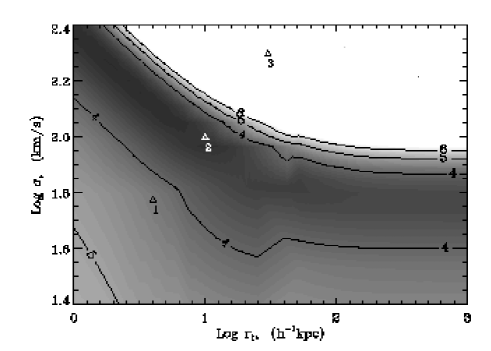
Figure 10: Upper panel : $\chi^{2}/{\rm dof}$ contour plot for the couple $(r_{t*},\sigma_{*})$. The “macro” model is the softened IS. Naturally, the $\chi^{2}$ minimum ($\sim 1.1$) is reduced as compared to the unperturbed previous model. The three peculiar couples 1, 2, 3 predict the fifth images plotted on the lower panel. The only noticeable effect of substructures on the fifth image occurs for models with a very high $\chi^{2}$ model that provide a bad fit for the external arcs.