Maximum-likelihood astrometric geometry calibration of interferometric telescopes: application to the Very Small Array

Abstract

Interferometers require accurate determination of the array configuration in order to produce reliable observations. A method is presented for finding the maximum-likelihood estimate of the telescope geometry, and of other instrumental parameters, astrometrically from the visibility timelines obtained from observations of celestial calibrator sources. The method copes systematically with complicated and unconventional antenna and array geometries, with electronic bandpasses that are different for each antenna radiometer, and with low signal-to-noise ratios for the calibrators. The technique automatically focusses on the geometry errors that are most significant for astronomical observation. We apply this method to observations made with the Very Small Array and constrain some $450$ telescope parameters, such as the antenna positions, effective observing frequencies and correlator amplitudes and phase shifts; this requires only $\sim 1$ h of CPU time on a typical workstation.

1 Introduction

Accurate knowledge of observing frequency, projected baselines and other geometric parameters is essential if interferometer data are to be turned into useful images. The accuracy required is typically a small fraction of the operating wavelength. For example, to keep phase errors below 10 degrees for an interferometer operating at 30 GHz, it is necessary to know the baseline length to an accuracy of better than 0.3 mm.

The standard way in which interferometer geometries are determined is along the following lines. First, direct measurements are made using, for example, tape measures, theodolites, and measurements of electrical lengths of electronic systems. Then, observations of celestial calibrators are carried out. For example, the observation by a particular pair of antennas of a bright calibrator of known RA and Dec gives the collimation phase of that pair (the difference in electrical length of the two arms of that interferometer). How this quantity varies, for example, with hour angle and for a series of calibrators at different declinations, is also investigated. These standard methods are described in e.g. Thompson, Moran & Swenson (1994), and in these ways a series of corrections to the directly measured geometry is produced, with the aim of ensuring that the physical baselines (in wavelengths) used in subsequent data analysis are correct.

This approach is of proven effectiveness for determining the geometries of interferometer arrays such as the Very Large Array (VLA). It is not adequate, however, for interferometers such as the Very Small Array (VSA, see e.g. Watson et al. (2002); Scott et al. (2002)), which is designed for imaging the CMB on scales $\ga 10$ arcmin at 30 GHz, and thus has baselines of length $\la 2$ m. At first sight this may seem surprising, as VSA baselines (in both metres and wavelengths) are so small. From the point of view of geometry determination from astrometry, however, the VSA is different from most other interferometer arrays in two respects.

• The collecting area of VSA antennas is very small and so there are few suitable celestial calibrators. Only the brightest calibrators are of use and signal-to-noise is a major issue.

• For most arrays like the VLA, the principal swivel axes of each antenna (e.g. altitude and azimuth, or polar and declination) intersect, at least nominally. If an axis is incorrectly aligned (e.g. the polar axis does not quite point to the Pole), then to first order this has no effect on the measured phase of a source, and its effect on source amplitude will manifest as a simple pointing correction which a standard 5-point observation (at expected source position, then offsets North, South, East then West) will provide. In the case of the VSA, the table elevation axis and the individual horn rotation axes (see Section 3) do not intersect by $\sim$ 1 m. This design helps reduce important systematic errors and also reduces cost, but it makes astrometric geometry determination significantly harder. If an axis is misaligned, then in general a phase error is also introduced. The identification of such errors is exacerbated by the lack of signal-to-noise.

There are also further difficulties associated with determining the geometry of the VSA, which can be present in other interferometers.

• As a result of, for example, the compliance needed for fitting horn-reflectors to cryostats, the position of the electrical centre of each horn will be slightly different, manifesting as a physical baseline correction and a pointing correction.

• A large observing bandwidth makes it hard to achieve a flat band pass, so the effective radio frequency becomes antenna dependent.

• Unconventional geometry makes it difficult to make a straightforward interpretation of a set of geometry calibration observations.

As a result of all these factors, phase (and amplitude) effects arise from complicated causes that are particularly hard to determine because of the lack of very high signal-to-noise calibrators. We have therefore implemented a maximum-likelihood method to determine the geometry, and other telescope parameters, astrometrically from the visibility timeline data obtained during a calibration observation of a sufficiently bright unresolved radio source. In the geometric model, we include as variables all the important dimensions and angles that require accurate determination, including the positions of the antennas, their effective observing frequencies and phase shifts on different baselines. In finding the best-fit geometry, the maximum-likelihood method correctly allows for the signal-to-noise ratio of the observations (on the assumption that the instrumental noise is Gaussian); the procedure also automatically guards against attempting to determine unimportant geometry errors that do not in fact much affect astronomical observation, since these similarly will not much affect calibrator observations.

In this paper, we focus on the method in its application to the VSA, although we point out the usefulness of the approach generally to radio and optical interferometry. In Section 2, we present the general maximum-likelihood method for the geometry calibration. The VSA is introduced in Section 3, where we develop a model of the telescope as a function of the parameters to be calibrated. Using this model, the likelihood method is applied to real VSA observations in Section 4. Finally, our conclusions are presented in Section 5.

2 Astrometric geometry calibration

Given a multi-dish interferometer consisting of $N_{a}$ separate antennas, with antenna positions denoted by ${\textbf{{d}}}_{i}$ ($i=1,\ldots,N_{a}$) relative to some origin, one can measure the correlated signals of any two antennas along $N_{b}=\frac{1}{2}N_{a}(N_{a}-1)$ independent baselines ${\textbf{{D}}}_{j}$ ($j=1,\ldots,N_{b}$), given in some ground-based reference frame specific to the telescope. The phase of the signal is modulated by the geometric path difference that the incident radiation experiences between the antennas. If the baseline is represented by a vector u in a coordinate system ($uv$-coordinates) such that the component $u$ of the vector ${\textbf{{u}}}=(u,v,w)$ is measured in the east-west direction, $v$ in the north-south direction and $w$ in the direction of the antennas’ pointing centre, the path difference is given by the projection of the direction cosines ${\textbf{{x}}}=(x,y,z)$ of the source on the sky onto the baseline components, i.e. by $\Delta={\textbf{{u}}}\cdot{\textbf{{x}}}$. Because the field of view is a section of a sphere, the third direction cosine is $z=\sqrt{1-x^{2}-y^{2}}$. Assuming a small field size or a sufficiently compact source, $z\approx 1$.

The response of an interferometer to an extended source can be obtained by integration over the solid angle of the source. Let us denote the sky brightness distribution of the source at the observing frequency $\nu$ by $I(x,y,\nu)$. One defines the complex (not fringe-rotated) visibility ${\cal V}(u,v,w,\nu)$ as (compare Thompson, Moran & Swenson, 1994)

$${\cal V}(u,v,w,\nu)=\int_{-\infty}^{\infty}\int_{-\infty}^{\infty}A(x,y,\nu)I(x,y,\nu)e^{2\pi i\frac{\nu}{c}(ux+vy+w)}{dx\ dy},$$ (1)

where $A(x,y,\nu)$ is the directional antenna (power) response pattern or primary beam (normalised to unity at its peak). To simplify the notation, we denote the real part $\Re[\mathcal{V}({\textbf{{u}}})]$ of the visibility $\mathcal{V}({\textbf{{u}}})$ by $\Re({\textbf{{u}}})$ and similarly $\Im({\textbf{{u}}})$ for the imaginary part.

For point sources at positions ${\textbf{{x}}}_{k}$ from the pointing centre, whose brightness distributions are given by $I({\textbf{{x}}})=S_{k}\ \delta({\textbf{{x}}}-{\textbf{{x}}}_{k})$, the integral (1) for the complex visibilities $\mathcal{V}({\textbf{{u}}},\nu)$ reduces to

$$\Re({\textbf{{u}}},\nu) = \sum_{k}A({\textbf{{x}}}_{k},\nu)S_{k}\cos\left(2\pi\frac{\nu}{c}{\textbf{{u}}}\cdot{\textbf{{x}}}_{k}\right),$$

$$\Im({\textbf{{u}}},\nu) = \sum_{k}A({\textbf{{x}}}_{k},\nu)S_{k}\sin\left(2\pi\frac{\nu}{c}{\textbf{{u}}}\cdot{\textbf{{x}}}_{k}\right),$$ (2)

where the sum is over all relevant sources in the field of view and ${\textbf{{x}}}_{k}$ and $S_{k}$ denote, for the $k$th source, respectively the position from the pointing centre and the flux.

As the Earth rotates, the u-vector corresponding to a baseline ${\textbf{{D}}}_{j}$ varies with the time $t_{i}$ at which the visibility sample was measured. We will denote the $uv$-coordinates of the $j$th baseline at a time $t_{i}$ (or alternatively at hour angle $H_{i}$) by ${\textbf{{u}}}_{ij}\equiv{\textbf{{u}}}({\textbf{{D}}}_{j},t_{i})$, and the corresponding visibility by $\mathcal{V}_{ij}$. The transformation ${\textbf{{R}}}(\delta,H_{i},L)$ that relates a baseline vector ${\textbf{{D}}}_{j}$ in the telescope frame to the $uv$-coordinates is a simple rotation given by

$${\textbf{{u}}}_{ij}={\textbf{{R}}}(\delta,H_{i},L)\ {\textbf{{D}}}_{j},$$ (3)

which will generally depend on the geographic latitude $L$ of the telescope and the declination $\delta$ and hour angle $H_{i}$ of the phase-tracking centre.

For a given a model of the telescope, the signal timelines for an observation of a point source can be predicted and compared with the observed data. If the source is sufficiently bright, one may then use a maximum-likelihood approach to determine the antenna geometry and a large number of other telescope parameters. For Gaussian instrumental noise the maximum-likelihood solution for the parameters can be found by minimising the standard $\chi^{2}$-misfit statistic between the predicted visibilities $\mathcal{V}^{\mathrm{P}}$ and observed visibilities $\mathcal{V}^{\mathrm{O}}$, namely

$$\chi^{2}(\mathcal{V}_{ij}^{\mathrm{P}},\mathcal{V}_{ij}^{\mathrm{O}}) = \sum^{N_{t},N_{b}}_{i,j}w_{ij}\ \left[(\Re^{\mathrm{O}}({\textbf{{u}}}_{ij})-\Re^{\mathrm{P}}({\textbf{{u}}}_{ij}))^{2}\right.$$ (4)

$$\qquad\,\,\quad\left.+(\Im^{\mathrm{O}}({\textbf{{u}}}_{ij})-\Im^{\mathrm{P}}({\textbf{{u}}}_{ij}))^{2}\right].$$

In this expression, the sums run over all $N_{t}$ time samples and $N_{b}$ baselines. The weights on the observed visibilities $\mathcal{V}_{ij}^{\mathrm{O}}$ are given by $w_{ij}=1/\sigma_{ij}^{2}$ assuming that the noises are independent, which is true for the thermal Johnson noises from each antenna. For a given observation, $\chi^{2}$ is a function of $N_{p}$ parameters $\{p_{l}\}$ ($l=1,\ldots,N_{p}$), including, for example, the antenna positions on the table $\{{\textbf{{d}}}_{i}\}$, the correlator amplitudes $\{C_{j}\}$, (constant) residual phase shifts $\{\phi_{j}\}$ and effective observing frequencies $\{\nu_{i}\}$. By minimising the $\chi^{2}$-function with respect to these parameters, it is possible to find the maximum-likelihood estimate of the telescope geometry.

Finding the global minimum of the $\chi^{2}$-function is numerically quite challenging. The optimisation takes place in an $N_{p}$-dimensional space and, as outlined for the VSA below, one typically has $N_{p}\approx 450$. Moreover, the $\chi^{2}=\mbox{constant}$ hypersurfaces are rather uneven. In particular, there are many local minima, and a straightforward (e.g. gradient search) minimisation algorithm may never find the correct basin of attraction. The existence of local minima can be understood intuitively, since a minimum occurs whenever the fringe pattern is fitted correctly on only one of the baselines. Even though the false minimum can easily be recognised from the poor fit on at least some of the timelines, a straightforward optimisation would stop there. Hence a successful fit requires a good initial estimate. Simulations show that for the VSA the initial antenna positions have to be measured manually to an accuracy of at least a third of a wavelength, i.e. roughly 3 mm. This is feasible with a steel tape measure. It should also be noted that there is a certain degeneracy in the problem. For example, a rescaling of the baselines is equivalent to a scaling of the observing frequency.

There are a number of possible numerical minimisation algorithms to choose from. Some of them employ gradient information, such as conjugate gradient algorithms (Press et al., 1992). Derivatives of the $\chi^{2}$-functional with respect to the telescope parameters can be found in Appendix A. Simulated annealing methods (Kirkpatrick et al., 1983) try to find their way through local minima. In this application, however, the number of parameters is very large and the $\chi^{2}$-surface does not have any significant large-scale slope, rendering a minimisation in a large number of dimensions very difficult even for the annealing method. Given a good initial estimate, we found a comparatively simple algorithm, Powell’s method (Press et al., 1992), to be very robust and reliable.

3 The Very Small Array

The VSA consists of an array of 14 horn-reflector antennas mounted at variable positions on a table that can be steered in elevation. The antennas track individually about their horn axes. A metallic enclosure serves as a ground shield. The observing frequency can be varied between 26 and 36 GHz, with a receiver bandwidth of 1.5 GHz and an effective system temperature of 30–35 K. The telescope was designed to be able to observe in two different configurations using antennas of different sizes.

1. The compact array consists of conical horn reflector antennas each with an aperture diameter of 14.3 cm. The primary beam has a FWHM of about $4.6\degr$ at a frequency of 34 GHz. The CMB power spectrum is measured in 10 independent bins of width $\Delta\ell\approx 80$ from $\ell\approx 100-900$. The VSA observed in the compact configuration between August 2000 and August 2001.

2. The extended array is a scaled version of the compact array. The aperture diameter is 32.2 cm, sampling multipoles $\ell\approx 350-1900$ with a resolution of $\Delta\ell\approx 200$. The VSA has been observing in the extended configuration since September 2001.

The table on which the VSA antennas are mounted can be tilted about a hinge aligned along the east-west direction (Fig. 1). The maximum elevation angle $\epsilon$ of the table is $70\degr$ and the minimum is $0\degr$. The antennas have an inclination relative to the table of $\eta=35\degr$ towards the south, allowing observations of up to $35\degr$ from the zenith to the north and south. Each antenna can individually track a source east-west up to angles of $\beta=40\degr$ from the meridian.

Figure 1: The VSA antennas are mounted on a table with a hinge in east-west direction, which tracks a source in elevation $\epsilon$. The individual horns are tilted at an angle $\eta$ with respect to the table and track in table ‘azimuth’ $\beta$.

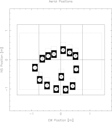
Figure 2: Top: the compact arrangement of the 14 VSA antennas on the table in September 2000. The rectangular area indicates the shape of the lower part of the VSA table, with the hinge on the lower end. The dashed lines above the horns show the extension of the antenna mount (Rusholme, 2001). Bottom: the $uv$-coverage of the VSA using the antenna arrangement shown in (a). The observed field is at a declination of $\delta=22\degr$. The duration of the observation is 3 hours either side of transit.

For the VSA, the rotation R from (3) is a function of the table elevation $\epsilon$. If the elevation has not been determined accurately, an error $\Delta\epsilon$ is introduced. Misalignments of the table hinge can be taken into account by polar angles $\theta$ and $\phi$ describing the deviation of the hinge from the east-west direction. Using the three-dimensional rotation matrices ${\textbf{{R}}}_{x}(\phi)$, ${\textbf{{R}}}_{y}(\phi)$ and ${\textbf{{R}}}_{y}(\phi)$ for right-handed rotations about the corresponding coordinate axes, R is given by

$${\textbf{{R}}}(\delta,H,L,\Delta\epsilon,\theta,\chi)$$ (5)

$$= {\textbf{{R}}}_{x}(\frac{\pi}{2}-\delta){\textbf{{R}}}_{z}(-H){\textbf{{R}}}_{x}(L-\frac{\pi}{2}){\textbf{{R}}}_{y}(\theta){\textbf{{R}}}_{z}(\chi){\textbf{{R}}}_{x}(\epsilon+\Delta\epsilon).$$

The actual arrangement of the antennas on the table for the compact configuration in September 2000 is shown in Fig. 2 (a). The resulting projected baselines during a 6-hour observation of a field at declination $\delta=22\degr$ are shown in panel (b). Since the telescope table is stationary with respect to the ground, during a track on a field the samples u lie on a series of curves (or $uv$-tracks).

Figure 3: Simplified schematic of the electronics of the receiving system of the VSA for compact array observations at a centre frequency of 33 GHz. A signal coming from an antenna at the radio frequency $\nu_{\mathrm{RF}}$ is reduced to the (2nd) IF frequency $\nu_{\mathrm{IF}}$ after mixing with the signals coming from the two local oscillators. It is split into $\sin$- and $\cos$-channels, and a geometric path delay is inserted into each channel separately. The correlated signals from pairs of antennas are integrated to produce the real and imaginary parts of the visibility.

The electronics of the receiving system of the VSA are illustrated in Fig. 3. An antenna receives a signal at the radio frequency $\nu_{\mathrm{RF}}$. After mixing with the two local oscillators, which produce a combined frequency $\nu_{\mathrm{LO}}=\nu_{\mathrm{LO},1}+\nu_{\mathrm{LO},2}$, the frequency of the signal is reduced to the (2nd) IF frequency $\nu_{\mathrm{IF}}=\nu_{\mathrm{RF}}-\nu_{\mathrm{LO}}$. In order to measure both the real and imaginary parts of the complex visibility, the signal is split into $\sin$- and $\cos$-channels with a phase difference of 90 degrees, yielding 28 such channels for $N_{a}=14$ antennas. To avoid a loss of signal coherence due to changing path lengths during a tracking run, appropriate geometric path delays are inserted into each channel. The correlated signals from each pair of antennas are integrated to produce the real and imaginary parts of the $N_{b}$ visibilities. To minimise the number of required splits of each $\cos$- or $\sin$-channel, the real part of the visibility for a given baseline can be formed from either the $\cos$-$\cos$ or the $\sin$-$\sin$ combinations, whereas the imaginary parts may consist of $\cos$-$\sin$ or $\sin$-$\cos$. A lookup table is used to determine which $\cos$- and $\sin$-channels correspond to real and imaginary parts of a given baseline.

The attenuation and passbands of filters and amplifiers are not spectrally flat, resulting in slightly different effective IF frequencies $\nu_{\mathrm{IF},\cos}$ and $\nu_{\mathrm{IF},\sin}$ for each antenna. Additional path delays introduced by the cables and electronics between antennas and correlators also affect the visibilities, and the amplitudes of the signal differ due to the different electronic gains of the correlators. Therefore the amplitudes $C^{(r)}_{j}$ and $C^{(i)}_{j}$ of the real and imaginary parts and phase shifts $\phi^{(r)}_{j}$ and $\phi^{(i)}_{j}$ vary for each baseline $j$. However, tests show that these are effectively constant over timescales of approximately one month on a given baseline.

The raw data have to be corrected for inserted path delays $\rho^{(r)}_{j,l}$ and $\rho^{(i)}_{j,l}$, where $l=1,2$ denotes the $\cos$ and $\sin$–channels from different antennas corresponding to the real and imaginary part of the $j$th baseline. The path delays are introduced at the different IF frequencies $\nu^{(r)}_{\mathrm{IF},j,l}$ and $\nu^{(i)}_{\mathrm{IF},j,l}$. Note that this notation with $2\times N_{b}$ different symbols obscures the fact that there are just $2\times N_{a}$ different path delays and IF frequencies, as the path delays are inserted per antenna and not per baseline.

Gathering together the effects described above, the predicted visibilities for the $j$th baseline for observations of a set of point sources at positions ${\textbf{{x}}}_{k}$ with fluxes $S_{k}$ are thus given by

$$\Re^{\mathrm{P}}({\textbf{{u}}}_{j}) = C^{(r)}_{j}\sum_{k}A\left({\textbf{{x}}}_{k},\sqrt{\nu^{(r)}_{j,1}\nu^{(r)}_{j,2}}\right)S_{k}$$

$$\times \cos\left(2\pi\left[\frac{\sqrt{\nu^{(r)}_{j,1}\nu^{(r)}_{j,2}}}{c}{\textbf{{u}}}_{j}\cdot{\textbf{{x}}}_{k}\right.\right.$$

$$\qquad-\left.\left.\left\{\frac{\nu^{(r)}_{\mathrm{IF},j,1}}{c}\rho^{(r)}_{j,1}-\frac{\nu^{(r)}_{\mathrm{IF},j,2}}{c}\rho^{(r)}_{j,2}\right\}+\phi^{(r)}_{j}\right]\right),$$

$$\Im^{\mathrm{P}}({\textbf{{u}}}_{j}) = C^{(i)}_{j}\sum_{k}A\left({\textbf{{x}}}_{k},\sqrt{\nu^{(i)}_{j,1}\nu^{(i)}_{j,2}}\right)S_{k}$$ (6)

$$\times \sin\left(2\pi\left[\frac{\sqrt{\nu^{(i)}_{j,1}\nu^{(i)}_{j,2}}}{c}{\textbf{{u}}}_{j}\cdot{\textbf{{x}}}_{k}\right.\right.$$

$$\qquad-\left.\left.\left\{\frac{\nu^{(i)}_{\mathrm{IF},j,1}}{c}\rho^{(i)}_{j,1}-\frac{\nu^{(i)}_{\mathrm{IF},j,2}}{c}\rho^{(i)}_{j,2}\right\}+\phi^{(i)}_{j}\right]\right),$$

where $\nu=\nu_{\mathrm{IF}}+\nu_{LO,1}+\nu_{LO,2}$ is the radio frequency corresponding to a given IF frequency $\nu_{\mathrm{IF}}$. The superscripts ^P indicate that the visibilities have been theoretically predicted. Given the calculable dependence of ${\textbf{{u}}}_{j}$ for each baseline on the time $t$, one can thus calculate the quantities $\mathcal{V}_{ij}^{\mathrm{P}}$ appearing in the expression for $\chi^{2}$ given in (4).

4 Analysis of VSA calibration observations

In order to constrain the geometry, an observation with a good signal-to-noise ratio at a sufficiently high elevation is required. There are three possible calibration sources for the VSA compact array that fulfil these requirements: Cas-A, Cyg-A and Tau-A. These are essentially unresolved point sources for the VSA compact array. In the plots presented below, we use a 4-h calibration observation of Cas-A as an illustrative example. The optimisation with respect to antenna positions, correlator amplitudes and phases and the IF frequencies was carried out using Powell’s algorithm down to a relative convergence tolerance of $10^{-3}$ in the value of $\chi^{2}$. The entire calculation required around 1 h of CPU time on a Sparc Ultra workstation.

4.1 Timelines

Figure 4: Comparison of observed and predicted fringes on VSA baseline antenna 1/antenna 2, using an observation of Cas-A. The panels show the real and imaginary parts, the amplitude and the phase of the visibility respectively, as a function of hour angle (in hours). The theoretical fringe predicted from the optimised telescope parameters is plotted with a solid line and the observed fringe with a dashed line. The units on the $y$-axis are arbitrary.

As an illustration of the fit obtained, in Fig. 4 we plot the observed fringes for VSA baseline antenna 1/antenna 2. The four panels show respectively the real and imaginary parts of the visibility, the amplitude and the phase, each as a function of hour angle. Each panel shows the timelines for the observed fringes (dashed) and the fringes predicted assuming the best-fit telescope geometry (solid), obtained from the $\chi^{2}$-minimisation. The scatter of the observed real and imaginary parts around the predicted lines indicates the noise level of the observation.

The quasi-sinusoidal fringe pattern shows an increasing fringe frequency for the 1/2 baseline. Since the data have not been fringe-rotated, the phase is going rapidly through cycles of $2\pi$. On this baseline, small quadrature errors (see Watson et al. (2002)) and differences in the amplitudes on the two channels are seen as a slight variation of the visibility amplitude and as structure in the visibility phase. We note that the best fit is in excellent agreement with the observations and matches the observed amplitudes and phases very closely.

4.2 The $\chi^{2}$-surface

Confirmation that the optimisation procedure has indeed fully converged can be seen in Fig. 5, 6 and 7. These plots show one-dimensional cuts through the $\chi^{2}$-surface in parameter space along some of the parameter coordinate axes. In each case, the $y$-axis indicates the value of the $\chi^{2}$-function, with an arbitrary normalisation, as a function of the deviation of the parameter value from the best-fit value. All plots are centred around a local minimum in the $\chi^{2}$-surface, indicating that the optimisation procedure has fully converged, and that the obtained reconstruction is indeed the maximum-likelihood estimate. There is, however, a strong caveat in interpreting these one-dimensional $\chi^{2}$-contours: they are by no means representative of the accuracy with which the parameters can be determined, which would require a marginalisation over all other parameters rather than a simple cut. In fact, the position and shape of the one-dimensional contour can be changed significantly by simply varying one or a few of the other parameters. To ensure that a minimum has been found, all parameters have to converge simultaneously.

Figure 5: The $\chi^{2}$-surface as a function of the $x$-position of VSA antenna 1. The units on the $x$-axis are metres from the optimised position, the $y$-units are arbitrary. Low values of $\chi^{2}$ correspond to the most likely solution. The minimisation has converged to the local minimum in the centre. A vertical line indicates the position of the manually measured value of the position.

Figure 6: The $\chi^{2}$-surface as a function of the $y$-position of antenna 1. Compare Fig. 5. It is interesting to note that adjacent minima are nearly as pronounced as the central one.

Figure 7: The $\chi^{2}$-surface as a function of the IF frequency on the $\cos$-channel of antenna 1. The $x$-axis is in units of 12 GHz from the optimal frequency, i.e. 0.01 corresponds to 120 MHz.

Fig. 5 shows a cut along the $x$-position of VSA antenna 1. Minima in $\chi^{2}$ correspond to the most likely solution. As for all other plots, the minimum has been found. A vertical line indicates the original input value of the position, as was manually measured on the table. Fig. 6 shows a cut along the $y$-position for the same antenna. It is obvious from the figure that, in this case, the calibration observation used is only just sufficient to distinguish between the true minimum and the adjacent minima either side, which are nearly as deep. As mentioned previously, to avoid being trapped in a false local minimum, one requires a sufficiently accurate initial estimate. Nevertheless, it is still possible to detect false minima, since the resulting positioning mistake of the order of 1 cm induces significant phase errors on at least one of the baselines of which the corresponding antenna is a part.

As a further illustration, Fig. 7 shows a cut along the IF frequency of the $\cos$-channel of antenna 1. Once more, we see that the position obtained by the Powell algorithm lies indeed at the minimum for this parameter.

4.3 Imaging with the VSA

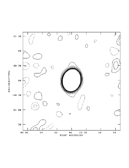
Figure 8: An image of Jupiter observed by the VSA. The geometry and other telescope parameters have been simultaneously calibrated by observations of Tau-A and Cas-A. The dynamical range of the image is 500:1, indicating that the phase errors due to the calibration are indeed negligible.

The parameters found from the calibration observations can be applied to the data reduction of subsequent observations. Fig. 8 shows a VSA map of Jupiter, which has been produced using a calibration that combined observations of both Cas-A and Tau-A. This highlights that the geometry fitting procedure can easily exploit several data sets simultaneously by simply adding up the $\chi^{2}$-functionals for all observations. The dynamical range of the image is an excellent 500:1, showing that the geometry calibration on other sources was sufficiently successful to render phase errors negligible. Other VSA maps are shown in Watson et al. (2002), and the primordial CMB maps obtained from VSA observations in the compact configuration are presented by Taylor et al. (2002).

5 Discussion and conclusions

In this paper, we have presented a method for astrometric geometry calibration of interferometers by performing a likelihood analysis of visibility timelines produced during an observation of a reasonably bright radio point source. The method has been demonstrated for the specific case of the Very Small Array, for which one must simultaneously constrain some 450 telescope parameters, such as the antenna positions, the effective observing frequency of each antenna which can vary due to different bandpass characteristics, and phase shifts on different baselines introduced in the electronic system or by different cable lengths. In particular, analysis of VSA observations of Tau-A and Cas-A sources show that the relative positions of the antennas on the telescope table can be determined to a small fraction of a wavelength. The quality of the fit is sufficiently good to enable high dynamic-range mapping with the VSA. This astrometric calibration is very straightforward and cheap, as it requires no equipment other than the telescope itself. Multiple calibration observations can easily be combined to produce a better parameter estimate by summing the $\chi^{2}$-functionals for all available data sets.

The calibration method is currently in active use by the VSA project and has successfully determined the geometry for several different antenna configuration since the start of its observing programme. The calibration of the VSA is described in more detail in Watson et al. (2002), and power spectra derived from the first year of observations in the compact configuration are presented in Scott et al. (2002).

Although the astrometric calibration method has been applied specifically to the VSA, it can easily be adapted to other telescopes. It is worth noting, however, that there is one feature of the VSA which does not necessarily generalise to other CMB telescopes, even though it is common to most ground-based arrays. Each VSA antenna tracks the source separately in ‘azimuth’ (semi-comounted design). This has the advantage of providing a valuable check on systematic contaminations, because the path delays on a particular baseline change during the observation and the sky signal can be recognised by its characteristic fringe frequency. On the Cosmic Background Imager (Padin et al., 2002) and the Degree Angular Scale Interferometer (Leitch et al., 2002), the antennas are mounted on a rigid tracking platform supported by an alt-azimuth mount. This design keeps the baseline projections with respect to the source constant and reduces the fringe rate on all baselines to zero, making the described geometry fitting impossible. A similar method can still be applied, however, if the fringe rate is artificially changed. For instance, the telescope could be kept at a fixed pointing position while the source is within the antenna beam, thus providing a non-zero fringe rate.

Appendix A Derivatives used in the VSA geometry calibration

For reference purposes, in this Appendix we quote the expressions for the derivatives of the $\chi^{2}$-functional (4) combined with the visibilities (6) used in the maximum-likelihood algorithm for the the VSA geometry calibration.

The gradient is required by some numerical minimisation algorithms that use gradient information to accelerate the computation. Although not required by the minimisation algorithm, the curvature can be useful for some iterative minimisation algorithms and for quantifying errors or uncertainties on the reconstruction. Assuming that the maximised estimate of the parameters is indeed in the correct basin of attraction on the likelihood surface and that this surface can be reasonably approximated by a Gaussian around the maximum, the uncertainties in the reconstruction can be obtained from the inverse of the Hessian matrix of $\chi^{2}$.

A.1 First derivatives of $\chi^{2}$

From (4), the $\chi^{2}$-gradient with respect to the telescope and correlator parameters $p_{l}$ is

$${\frac{\partial\chi^{2}}{\partial p_{l}}} = 2\sum^{N_{t},N_{b}}_{i,j}w_{ij}\left[\left(\Re^{\mathrm{P}}({\textbf{{u}}}_{ij})-\Re^{\mathrm{O}}({\textbf{{u}}}_{ij})\right){\frac{\mathrm{d}\Re^{\mathrm{P}}({\textbf{{u}}}_{ij})}{\mathrm{d}p_{l}}}+\left(\Im^{\mathrm{P}}({\textbf{{u}}}_{ij})-\Im^{\mathrm{O}}({\textbf{{u}}}_{ij})\right){\frac{\mathrm{d}\Im^{\mathrm{P}}({\textbf{{u}}}_{ij})}{\mathrm{d}p_{l}}}\right]$$

where again the symbol $\Re^{\mathrm{P}}({\textbf{{u}}}_{ij})$ denotes the real part of the visibility predicted for the $i$th time sample on the $j$th baseline. The dependence of the visibilities on the parameters can be explicit, as in the case of the correlator amplitudes, or implicit in the position of the samples ${\textbf{{u}}}_{ij}$, as for the antenna positions:

$${\frac{\mathrm{d}\Re^{\mathrm{P}}({\textbf{{u}}}_{ij})}{\mathrm{d}p_{l}}}={\frac{\partial\Re^{\mathrm{P}}({\textbf{{u}}}_{ij})}{\partial p_{l}}}+{\frac{\partial\Re^{\mathrm{P}}({\textbf{{u}}}_{ij})}{\partial{\textbf{{u}}}_{ij}}}\cdot{\frac{\partial{\textbf{{u}}}_{ij}}{\partial p_{l}}}.$$ (7)

We now substitute the expressions (6) appropriate for the VSA. For the sake of notational brevity, we define the arguments

$$\psi^{(r)} = \frac{\sqrt{\nu^{(r)}_{1}\nu^{(r)}_{2}}}{c}{\textbf{{u}}}_{j}\cdot{\textbf{{x}}}_{k}-\left\{\frac{\nu^{(r)}_{\mathrm{IF},1}}{c}\rho^{(r)}_{1}-\frac{\nu^{(r)}_{\mathrm{IF},2}}{c}\rho^{(r)}_{2}\right\}+\phi^{(r)},$$

$$\nu^{(r)} = \sqrt{\nu^{(r)}_{1}\nu^{(r)}_{2}},$$ (8)

and similarly for $\psi^{(i)}$ and $\nu^{(i)}$. Then the derivatives of the predicted visibilities with respect to the $uv$-loci,

$${\frac{\partial\Re^{\mathrm{P}}({\textbf{{u}}})}{\partial{\textbf{{u}}}}} = -2\pi C^{(r)}\sum_{k}A({\textbf{{x}}}_{k},\nu^{(r)})S_{k}\sin\left(2\pi\psi^{(r)}\right)\frac{\nu^{(r)}}{c}{\textbf{{x}}}_{k},$$

$${\frac{\partial\Im^{\mathrm{P}}({\textbf{{u}}})}{\partial{\textbf{{u}}}}} = 2\pi C^{(i)}\sum_{k}A({\textbf{{x}}}_{k},\nu^{(i)})S_{k}\cos\left(2\pi\psi^{(i)}\right)\frac{\nu^{(i)}}{c}{\textbf{{x}}}_{k},$$

only depend on table parameters, whereas

$${\frac{\partial\Re^{\mathrm{P}}({\textbf{{u}}})}{\partial C^{(r)}}} = \sum_{k}A({\textbf{{x}}}_{k},\nu^{(r)})S_{k}\cos\left(2\pi\psi^{(r)}\right),$$

$${\frac{\partial\Im^{\mathrm{P}}({\textbf{{u}}})}{\partial C^{(i)}}} = \sum_{k}A({\textbf{{x}}}_{k},\nu^{(i)})S_{k}\sin\left(2\pi\psi^{(i)}\right),$$ (10)

$${\frac{\partial\Re^{\mathrm{P}}({\textbf{{u}}})}{\partial\phi^{(r)}}} = -2\pi C^{(r)}\sum_{k}A({\textbf{{x}}}_{k},\nu^{(r)})S_{k}\sin\left(2\pi\psi^{(r)}\right),$$

$${\frac{\partial\Im^{\mathrm{P}}({\textbf{{u}}})}{\partial\phi^{(i)}}} = 2\pi C^{(i)}\sum_{k}A({\textbf{{x}}}_{k},\nu^{(i)})S_{k}\cos\left(2\pi\psi^{(i)}\right),$$ (11)

only depend on parameters of the electronic system.

The derivatives with respect to the frequencies are

$${\frac{\partial\Re^{\mathrm{P}}({\textbf{{u}}})}{\partial\nu^{(r)}_{\mathrm{IF},1}}} = -2\pi C^{(r)}\sum_{k}A({\textbf{{x}}}_{k},\nu^{(r)})S_{k}\sin\left(2\pi\psi^{(r)}\right)\left(\frac{1}{2c}\sqrt{\frac{\nu^{(r)}_{2}}{\nu^{(r)}_{1}}}-\frac{\rho^{(r)}_{1}}{c}\right){\textbf{{u}}}_{j}\cdot{\textbf{{x}}}_{k},$$

$${\frac{\partial\Re^{\mathrm{P}}({\textbf{{u}}})}{\partial\nu^{(r)}_{\mathrm{IF},2}}} = -2\pi C^{(r)}\sum_{k}A({\textbf{{x}}}_{k},\nu^{(r)})S_{k}\sin\left(2\pi\psi^{(r)}\right)\left(\frac{1}{2c}\sqrt{\frac{\nu^{(r)}_{1}}{\nu^{(r)}_{2}}}+\frac{\rho^{(r)}_{2}}{c}\right){\textbf{{u}}}_{j}\cdot{\textbf{{x}}}_{k},$$

and analogously for the imaginary parts. These derivatives apply to a single baseline only. In practice, a given frequency channel is used in several baselines. In order to compute the $\chi^{2}$-derivatives one thus has to sum over all baselines containing the respective frequency channel.

The derivatives of the $uv$-positions with respect to the geometric parameters are given by

$${\frac{\partial(u_{ij})_{k}}{\partial p_{l}}}=\left\{\begin{array}[]{ll}\sum_{m}{\frac{\partial R^{i}_{km}}{\partial p_{l}}}D^{j}_{m}&\quad\mbox{if $p_{l}\in\{\Delta\epsilon,\theta,\phi\}$}\\ \sum_{m}R^{i}_{km}{\frac{\partial D^{j}_{m}}{\partial p_{l}}}&\quad\mbox{if $p_{l}\in\{{\textbf{{d}}}_{i}\}$}\\ 0\phantom{{\frac{\partial D^{j}_{m}}{\partial p_{l}}}}&\quad\mbox{otherwise}\end{array}\right.,$$ (13)

where subscripts denote the vector components, D is a baseline vector and ${\textbf{{R}}}(\delta,H_{i},L,\Delta\epsilon,\theta,\chi)$ is the transformation matrix from table to $uv$-coordinates introduced in (5):

$${\textbf{{u}}}_{ij}={\textbf{{R}}}(\delta,H,L,\Delta\epsilon,\theta,\chi)\ {\textbf{{D}}}_{j}(\{{\textbf{{d}}}_{i}\}).$$

Derivatives with respect to parameters other than the table parameters will vanish since they do not affect the geometry. Furthermore, a given baseline depends only on the positions of those two horns of which it is composed, and the resulting matrix is considerably sparse.

A.2 Curvature of $\chi^{2}$

Denoting the real part of the visibility predicted at the $i$th time sample on baseline $j$ by $\Re^{\mathrm{P}}_{ij}$, the $\chi^{2}$-curvature is given by

$${\frac{\partial^{2}\chi^{2}}{\partial p_{l}\partial p_{n}}} = 2\sum_{i,j}w_{ij}\left\{\left({\frac{\partial\Re^{\mathrm{P}}_{ij}}{\partial{\textbf{{u}}}}}\cdot{\frac{\partial{\textbf{{u}}}_{ij}}{\partial p_{n}}}\right)\left({\frac{\partial\Re^{\mathrm{P}}_{ij}}{\partial p_{l}}}+{\frac{\partial\Re^{\mathrm{P}}_{ij}}{\partial{\textbf{{u}}}}}\cdot{\frac{\partial{\textbf{{u}}}_{ij}}{\partial p_{l}}}\right)\right.$$

$$+\left(\Re^{\mathrm{P}}_{ij}-\Re^{\mathrm{O}}_{ij}\right)\ \left[{\frac{\partial^{2}\Re^{\mathrm{P}}_{ij}}{\partial p_{l}\partial p_{n}}}+\left({\frac{\partial{\textbf{{u}}}_{ij}}{\partial p_{n}}}\right)^{\mathrm{t}}\left[\nabla_{{\textbf{{u}}}}\nabla_{{\textbf{{u}}}}\Re^{\mathrm{P}}_{ij}\right]\left({\frac{\partial{\textbf{{u}}}_{ij}}{\partial p_{l}}}\right)+{\frac{\partial\Re^{\mathrm{P}}_{ij}}{\partial{\textbf{{u}}}}}\cdot{\frac{\partial^{2}{\textbf{{u}}}_{ij}}{\partial p_{l}\partial p_{n}}}\right]$$

$$+\left({\frac{\partial\Im^{\mathrm{P}}_{ij}}{\partial{\textbf{{u}}}}}\cdot{\frac{\partial{\textbf{{u}}}_{ij}}{\partial p_{n}}}\right)\left({\frac{\partial\Im^{\mathrm{P}}_{ij}}{\partial p_{l}}}+{\frac{\partial\Im^{\mathrm{P}}_{ij}}{\partial{\textbf{{u}}}}}\cdot{\frac{\partial{\textbf{{u}}}_{ij}}{\partial p_{l}}}\right)$$

$$+\left.\left(\Im^{\mathrm{P}}_{ij}-\Im^{\mathrm{O}}_{ij}\right)\ \left[{\frac{\partial^{2}\Im^{\mathrm{P}}_{ij}}{\partial p_{l}\partial p_{n}}}+\left({\frac{\partial{\textbf{{u}}}_{ij}}{\partial p_{n}}}\right)^{\mathrm{t}}\left[\nabla_{{\textbf{{u}}}}\nabla_{{\textbf{{u}}}}\Im^{\mathrm{P}}_{ij}\right]\left({\frac{\partial{\textbf{{u}}}_{ij}}{\partial p_{l}}}\right)+{\frac{\partial\Im^{\mathrm{P}}_{ij}}{\partial{\textbf{{u}}}}}\cdot{\frac{\partial^{2}{\textbf{{u}}}_{ij}}{\partial p_{l}\partial p_{n}}}\right]\right\}.$$

Again the expressions (LABEL:eqn:geochi2gradu)–(LABEL:eqn:geochi2gradfreq) can be used to substitute for the partial derivatives.

References

- Kirkpatrick et al. (1983) Kirkpatrick S., Gelatt Jr. C.D., Vecchi M.P., 1983, Science, 220, 671
- Leitch et al. (2002) Leitch E.M., 2002, ApJ, 568, 28
- Padin et al. (2002) Padin S. et al., 2002, PASP, 114, 83
- Press et al. (1992) Press W.H., Teukolsky S.A., Vetterling W.T., Flannery B.P., 1992, Numerical Recipies in Fortran. CUP, Cambridge
- Rusholme (2001) Rusholme B., 2001, The Very Small Array. PhD thesis, University of Cambridge
- Scott et al. (2002) Scott P.F. et al., 2002, submitted to MNRAS, astro-ph/0205380
- Taylor et al. (2002) Taylor A.C. et al., 2002, submitted to MNRAS, astro-ph/0205381
- Thompson, Moran & Swenson (1994) Thompson A.R., Moran J.M., Swenson G.W., 1994, Interferometry and Synthesis in Radio Astronomy. Krieger Publishing Company, New York
- Watson et al. (2002) Watson R.A. et al., 2002, submitted to MNRAS, astro-ph/0205378