Cosmic Crystallography of the Second Order

Abstract

The cosmic crystallography method of Lehoucq et al. [1] produces sharp peaks in the distribution of distances between the images of cosmic sources. But the method cannot be applied to universes with compact spatial sections of negative curvature. We apply to the these a second order crystallographic effect, as evidenced by statistical parameters.

PACS number: 98.80.Jk

Keywords: cosmology, large scale structure

1 Introduction

The method of cosmic crystallography was developed by Lehoucq, Lachièze-Rey, and Luminet [1], and consists of plotting the distances between cosmic images of clusters of galaxies. In Euclidean spaces, we take the square of the distance between all pairs of images on a catalogue versus the frequency of occurence of each of these distances. In universes with Euclidean multiply connected spatial sections, we have sharp peaks in a plot of distance distributions.

It is usual to consider the Friedmann-Lemaître-Robertson-Walker (FLRW) cosmological models of constant curvature $(S^{3},E^{3},H^{3})$ with simply connected spatial sections. However, models with these spacetime metrics also admit, compact, orientable, multiply connected spatial sections, which are represented by quotient manifolds $M=\tilde{M}/\Gamma$, where $\tilde{M}$ is $S^{3}$, $E^{3}$ or $H^{3},$ and $\Gamma$ is a discrete group of isometries (or rigid motions) acting freely and properly discontinously on $\tilde{M}$. The manifold $M$ is described by a fundamental polyhedron (FP) in $\tilde{M}$, with faces pairwise identified through the action of the elements of $\Gamma$. So $\tilde{M}$ is the universal covering space of $M$ and is the union of all cells $g($FP$)$, $g\in$ $\Gamma$.

The repeated images of a cosmic source is the basis of the cosmic cristallography method. The images in a multiply connected universe are connected by the elements $g$ of $\Gamma$. The distances between images carry information about these isometries. These distances are of two types [2]: type I pairs are of the form $\{g(x),g(y)\},$ where

$$distance[g(x),g(y)]=distance[x,y],$$ (1)

for all points $x,y\in M$ and all elements $g\in$ $\Gamma$; type II pairs of the form $\{x,g(x)\}$ if

$$distance[x,g(x)]=distance[y,g(y)],$$ (2)

for at least some points $x,y\in M$ and some elements $g$ of $\Gamma$.

The cosmic cristallography method puts in evidence type II pairs. These distances are due to Clifford translations, which are elements $g\in\Gamma,$ such that Eq. (2) holds for any two points $x,y\in M.$ Type II pairs give sharp peaks in distance distributions in Euclidean [1, 3] and spherical spaces [4], but they do not appear in hyperbolic space. This is illustrated in Fig. 1 for an FLRW model with total energy density $\Omega_{0}=0.3$ and having as spatial sections the Weeks manifold - coded $m003(-3,1)$ in [5] and in Table I below - which is the closed, orientable hyperbolic manifold with the smallest volume (normalized to minus one curvature) known. The Bernui-Teixeira (B-T) function [6] is an analytical expression for a uniform density distribution in an open hyperbolic model.

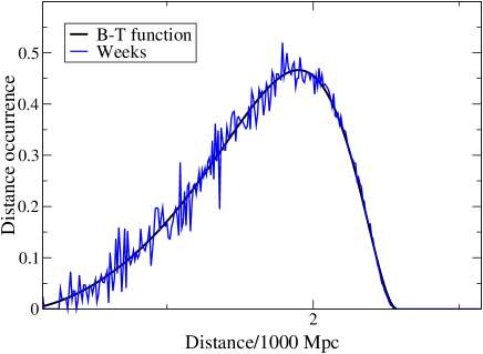
Figure 1: Distribution of pair distances of cosmic images for the Bernui-Teixeira function, and for a universe with Weeks manifold as spatial sections and $\Omega_{0}=0.3.$

In hyperbolic spaces, the identity (or trivial motion) is the only Clifford translation. In this case, the cosmic cristallography method by itself cannot help us to detect the global topology of the universe. Several works have tried to identify multiply connected, or closed, hyperbolic universes by applying variants of the cosmic cristallographical method [7, 8, 9, 10], most of which now rely on type I, in the absence of type II, isometries. It is these variants that we call cosmic crystallography of the second degree.

One of these [7], proposed by us, consisted of subtracting, from the distribution of distances between images in closed hyperbolic universes, the similar distribution for the open model. It did not pretend to be useful for the determination of a specific topology, but it might reinforce other studies that look for nontrivial topologies.

Uzan, Lehoucq, and Luminet [9] invented the collect correlated pairs method, that collect type I pairs and plot them so as to produce one peak in function of the density parameters, $\Omega_{m}$ for matter and $\Omega_{\Lambda}$ for dark energy.

Gomero et al. [10] obtained topological signatures, by taking averages of distance distributions for a large number of simulated catalogues and subtracting from them averages of simulations for trivial topology.

Here we introduce still another second order crystallographic method, in the absence of Clifford translations and sharp peaks. We look for signals of nontrivial topology in statistical parameters of their distance distributions.

As commented above on Ref. [7], these methods are not as powerful as the original Clifford crystallography, but will certainly be useful as added tools to help looking for the global shape of the universe.

2 Simulations

Let the metric of the Friedmann’s open model be written as

$$ds^{2}=a^{2}(\eta)(d\eta^{2}-d\lambda^{2})\ ,$$ (3)

where $a(\eta)$ is the expansion factor or curvature radius, and

$$d\lambda^{2}=d\chi^{2}+\sinh^{2}\chi(d\theta^{2}+\sin^{2}\theta\,d\phi^{2})$$ (4)

is the standard metric of hyperbolic space $H^{3}$. We assume a null cosmological quantity, hence the expressions for $a(\eta)$ and other quantities are as in Friedmann’s open model - see, for example, Landau and Lifshitz [11].

To simulate our catalogues we assume for the cosmological density parameter the values $\Omega_{0}=0.3$ and $\Omega_{0}=0.4,$ with Hubble’s constant $H_{0}=65\,$km s^-1Mpc^-1. The present value of the curvature radius is $a(\eta_{0})=5513$ Mpc for $\Omega_{0}=0.3$ and $5954\,$Mpc for $\Omega_{0}=0.4$.

To generate pseudorandom source distributions in the FP, we first change the coordinates to get a uniform density in coordinate space:

$$dV=\sinh^{2}\chi\sin\theta\,\,d\chi\,d\theta\,d\phi=du\,dv\,d\phi\,,$$

with $u(\chi)=(\sinh\chi\cosh\chi-\chi)/2$ and $v(\theta)=\cos^{-1}\theta$. Our sources are then generated with equal probabilities in $(u,v,\phi)$ space, and their large scale distributions are spatially homogeneous.

Table I. The eight manifolds used as spatial sections. Their names and
data are taken from the SnapPea software. The last two columns give
a number of cells that cover the observable universe.
Manifold				Number of cells
Name	Volume	$\chi_{in}$	$\chi_{out}$	$\Omega_{0}=0.3$	$\Omega_{0}=0.4$
m003(-3,1)	0.94	0.52	0.75	747	379
m003(-2,3)	0.98	0.54	0.75	729	357
m017(-3,2)	1.89	0.64	0.85	463	247
m221(+3,1)	2.83	0.74	0.94	403	199
m342(-4,1)	3.75	0.77	1.16	451	237
s890(+3,2)	4.69	0.87	1.38	653	273
v2051(+3,2)	4.69	0.87	1.38	653	273
v2293(+3,2)	4.69	0.87	1.38	653	273

We did the simulations for eight spatially compact, hyperbolic models. Their space sections are the manifolds listed in Table I, which gives their names, volumes, and the circumscribing and inscribing radii ($\chi_{out}$ and $\chi_{in}$) of their FP’s. These and other data on the manifolds were obtained from the SnapPea program [5]. In the last two columns, we list the number of cells (replicas of FP) needed to assure a complete cover  of $H^{3}$ up to a radius $\chi=2.335$ for $\Omega_{0}=0.3$ and $\chi=1.996$ for $\Omega_{0}=0.4$. This corresponds to the redshift ($Z=1300$) of the last scattering surface. Aproximately $850$ images were created in each simulated catalogue. Manifolds with different volumes will have different numbers of sources in their FP’s.

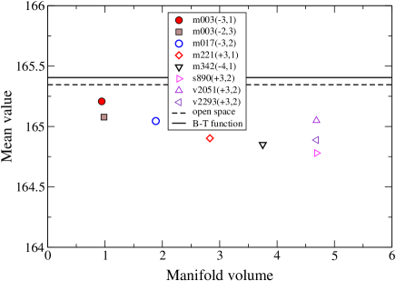
Figure 2: The mean values for the eight studied manifolds, with $\Omega_{0}=0.3.$ In this and remaining figures, a dashed line marks the value of the plotted parameter for the open model, and a solid line marks the Bernui-Teixeira value.

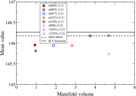
Figure 3: The mean values for our simulations with $\Omega_{0}=0.4$.

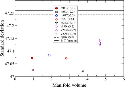
Figure 4: The standard deviations $\sigma$ for the simulations with $\Omega_{0}=0.3.$

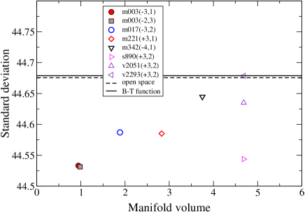
Figure 5: The standard deviations for $\Omega_{0}=0.4.$

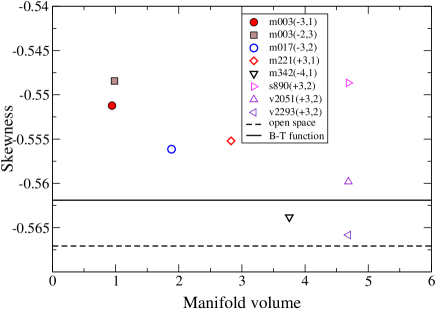
Figure 6: The skewnesses for $\Omega_{0}=0.3$.

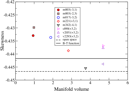
Figure 7: The skewnesses for $\Omega_{0}=0.4$.

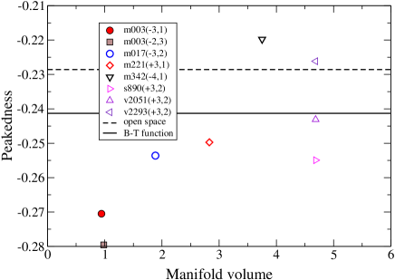
Figure 8: The peakednesses for $\Omega_{0}=0.3.$

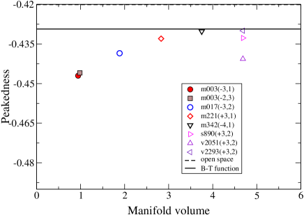
Figure 9: The peakednesses for $\Omega_{0}=0.4.$

Ten different pseudorandom distributions of sources for each manifold were simulated. From the result of each simulation we calculated the distance distribution and then the latter’s mean value $mv=E[X],$ standard deviation $\sigma=\sqrt{\mu_{2}},$ skewness $sn=\mu_{3}/\sigma^{3},$ and peakedness $pn=(\mu_{4}/\sigma^{4})-3,$ where $X$ is the distance variable, $E$ is the expected value operator, and $\mu_{\nu}=E[(X-mv)^{\nu}]$ is the $\nu$-moment about the mean value - cf. [12], for example.

For each of our chosen eight compact manifolds, we took the averages of these statistical parameters for ten simulations (obtained by varying the computer pseudorandom seed), to get their tendency in comparison with those for the simply connected case.

We proceeded in two ways to obtain a distribution in the open model, for comparison with the compact cases. In one of them, a simulated catalogue (real ones are not yet deep enough for use in cosmic crystallography) was obtained, with the same cosmological parameters and a pseudorandom distribution of sources inside the observable universe (redshift $\leq 1300$). In the other, the analytical Bernui-Teixeira function for a uniform distribution in simply connected universes [6] was used.

3 Results and conclusions

We compare the results for eight compact manifolds with those for the simulated simply connected case, and with the B-T function. Figures 2-9 show these results for $mv$, $\sigma$, $sn$, and $pn$, plotted vs. the manifold volumes, with the density parameters $\Omega_{0}=0.3$ and $\Omega_{0}=0.4$. It is of course premature to think of a functional dependence on volume (except for the obvious fact that, if the volume is so large as to enclose the observable universe, then the distribution of sources is indistinguishable from that for an open universe - see Fagundes [13], for example). But we note a tendency of $mv$, $\sigma$, and $pn$ in compact universes to have values below those of the corresponding B-T function, and for $sn$ to lie above that function. This could give us a signal of nontrivial topology in a future, realistic situation.

We expect that the presence of type I pairs of distances is more evident for manifolds with smaller normalized volumes, or for models with smaller $\Omega_{0}$. In fact our results are better for $mv$ and $\sigma$ with $\Omega_{0}=0.3$, where the observable universe is bigger than for $\Omega_{0}=0.4$. This implies more copies of the FP, and hence more topological effects. The set of these statistical parameters may eventually provide a complementary indication as for the multiply connectedness of a possibly negatively curved cosmos.

E. G. is grateful to Fundação de Amparo à Pesquisa do Estado de São Paulo (FAPESP Process 01/10328-6) for a post-doctoral scholarship. H. V. F. thanks Conselho Nacional de Desenvolvimento Científico e Tecnológico (CNPq Process 300415/84-2) for partial financial support.

References

- [1] R. Lehoucq, M. Lachièze-Rey, and J.-P. Luminet, Astron. Astrophys. 313, 339 (1996).
- [2] J.-P. Uzan, R. Lehoucq and J.-P. Luminet, Astron. Astrophys. 344, 735 (1999).
- [3] H. V. Fagundes and E. Gausmann, Phys. Lett. A238, 235 (1998).
- [4] E. Gausmann, R. Lehoucq, J.-P. Luminet, J.-P. Uzan, and J. R. Weeks, Class. Quantum Grav. 18, 5155 (2001).
- [5] J. R. Weeks, SnapPea: A Computer Program for Creating and Studying Hyperbolic Manifolds, available at Web site www.northnet.org/weeks.
- [6] A. Bernui and A. F. F. Teixeira, Cosmic Crystallography: Three Multipurpose Functions, astro-ph/9904180.
- [7] H. V. Fagundes and E. Gausmann, astro-ph/9811368; Proc. XIX Texas Symp. Rel. Astrophys. Cosmology, CD-ROM version.
- [8] H. V. Fagundes and E. Gausmann, Phys. Lett. A261, 235 (1999).
- [9] J.-P. Uzan, R. Lehoucq, and J.-P. Luminet, Astron. Astrophys. 351, 766 (1999).
- [10] G. I. Gomero, M. J. Rebouças, and A. F. F. Teixeira, Int. J. Mod. Phys. D9, 687 (2000).
- [11] L. Landau and E. Lifshitz, The Classical Theory of Fields (Addison-Wesley, Reading, 1961).
- [12] J. W. Barnes, Statistical Analysis for Engineers and Scientists (McGraw-Hill, New York, 1994).
- [13] H. V. Fagundes, Phys. Rev. Letters 51, 517 (1983).