X-RAY EMISSION OF YOUNG SN IA REMNANTS
AS A PROBE FOR AN EXPLOSION MODEL

Abstract

We present results of hydrodynamical simulations of young supernova remnants. To model the ejecta, we use several models (discussed in literature) of type Ia supernova explosions with different abundances. Our hydro models are one-dimensional and spherically symmetrical, but they take into account ionization kinetics with all important processes. We include detailed calculations for the X-ray emission, allowing for time-dependent ionization and recombination. In particular, we compare the computed X-ray spectra with recent XMM-Newton observations of the Tycho SN remnant. Our goal is to find the most viable thermonuclear SN model that gives good fits to both these X-ray observations and typical SN Ia light curves.

Introduction

Recent observations with XMM-Newton telescope with high spectral and space resolution, give us an opportunity to get clearer understanding of nature and origin of X-ray sources. For example, with new data on supernova remnants we can find out more about the supernova explosion itself. So far, there exist many explosion models proposed by theorists for different types of supernovae, but still there are no definite criteria to decide which of the models are realized in nature. During the first months after an explosion one can examine a theoretical model by calculating bolometric and monochromatic light curves and spectra. Later on, gas in the ejecta cools down and becomes almost unobservable. The next opportunity to analyze the ejecta is on the stage of a young supernova remnant (SNR), when noticeable amount of circumstellar gas is swept up. At this moment a reverse shock forms, goes inwards the ejecta and illuminates it once again.

We will focus only on Type Ia Supernovae (SN Ia) and compare the results for four theoretical models of explosion. We are eager to find a model which would be in good agreement with observations of SN Ia both at the epoch of maximum light and on the young remnant stages.

In this work, we calculate hydrodynamical evolution and X-ray emission of a supernova remnant at the age of 430 years, which corresponds to the age of Tycho SNR, and compare the results with spectra and images of this remnant obtained by XMM-Newton space telescope (Decourchelle et al. 2001). We examine the same models that where applied to our broad-band light curve modelling (Blinnikov, Sorokina 2003), so we will be able to judge on the correctness of these models from two points of view.

Quite a while ago, it was concluded that Tycho’s supernova was of Type I (Baade 1945). After that time there were many other papers which suggested other types for Tycho. But the morphology of the remnant, its shell-like structure, says that most probably it is still the remnant of Type Ia supernova.

The basic parameters of the Tycho remnant are the following: the age is 430 years, the angular size is $\sim 8^{\prime}$, thus the radius is $\sim 2-3$ pc (depending on adopted distance). It has almost spherical shape, so we do not need any additional assumptions to model it with a 1D code.

Tycho’s remnant was observed for many years in radio wavelength and optics with terrestrial instruments (e.g., van den Bergh 1971, van den Bergh et al. 1973, Duin, Strom 1975, Dickel et al. 1982) and in X-rays with different space telescopes (e.g., Davison et al. 1976, Seward et al. 1983, Tsunemi et al. 1986, Hwang, Gotthelf 1997, Decourchelle et al. 2001). Its images and spectra were analyzed in many papers (e.g., Chevalier, Raymond 1978, Hamilton et al. 1986, Itoh et al. 1988, Brinkmann et al. 1989, Vancura et al. 1995, Hwang et al. 1998). The instruments become better every decade. The most recent observations with XMM-Newton provide us with data of excellent spatial resolution, which allows us to examine not only crude models to reproduce the emission of the remnant, but also to change between models which differ not very strongly.

Models

To simulate supernova ejecta in our calculations of evolution and X-ray emission of remnant we have chosen four SN Ia explosion models. Three of them are Chandrasekhar-mass models and one is a sub-Chandrasekhar one:

• the classical deflagration model W7 (Nomoto et al. 1984). $M_{WD}=1.38M_{\odot}$, $E_{0}=1.2\times 10^{51}$ ergs, M(⁵⁶Ni) $=0.6M_{\odot}$.

• the deflagration model by Reinecke et al. (2002) (hereafter MR0). $M_{WD}=1.38M_{\odot}$, $E_{0}=4.6\times 10^{50}$ ergs, M(⁵⁶Ni) $=0.43M_{\odot}$.

• the delayed detonation model DD4 (Woosley & Weaver 1994b). $M_{WD}=1.38M_{\odot}$, $E_{0}=1.2\times 10^{51}$ ergs, M(⁵⁶Ni) $=0.6M_{\odot}$.

• the sub-Chandrasekhar-mass detonation model with low ⁵⁶Ni production (hereafter, WD065; Ruiz-Lapuente et al. 1993). $M_{WD}=0.65M_{\odot}$, $E_{0}=5.6\times 10^{50}$ ergs, M(⁵⁶Ni) $=0.5M_{\odot}$.

W7, DD4, and WD065 are well known SN Ia models. The last one is the best for modelling light curves and late spectra of very sub-luminous SNe Ia, like 1991bg. Two others are usually considered as the best models for typical SN Ia.

The recent MR0 model is originally 3D, but we have averaged it over the whole $4\pi$, since our hydro code is 1D. MR0 is almost a “first principle” model, and uses much less free parameters for flame modelling than all previous calculations. It is less energetic, contains less ⁵⁶Ni, but the latter is located in the outermost layers of ejecta due to 3D Rayleigh–Taylor instability. The combination of all these factors leads to the situation when the outermost ⁵⁶Ni layer has similar velocities for all Chandrasekhar-mass models.

From our light curve modelling (Blinnikov, Sorokina 2003) we have found that MR0 model is the best for UBVI bands, though the bolometric light curve is more similar to observations for W7. We discussed there that a bit more energetic model, and equally mixed as MR0, would be the best from the light curve modelling point of view.

We surround ejecta by a motionless gas of constant density ($5\times 10^{-24}\mbox{ g/cm}^{3}$), constant temperature ($10^{4}$ K), and with Solar abundances. We start calculations of the remnant evolution at the age of ejecta from several years to several decades.

Method

To model the hydrodynamical evolution of the supernova remnant we use hydro code from the package STELLA (Blinnikov et al. 2000). To find out the X-ray spectra we use the code written by P.L. for calculations of collisional ionization of a stationary plasma, which takes into account basic processes: ionization by electron impact, autoionization, photorecombination, dielectronic recombination, charge transfer. It calculates bremsstrahlung (free-free), free-bound, bound-bound, two-photon emission. This code has been elaborated by S.B. and E.S. into a time-dependent variant ($\dot{n}_{i}=f(T(t),n(t),Z,...)$ for all ionic species). Input parameters are current temperature, density, abundance.

The models were calculated as follows. We simulate an SN expansion into CSM, assuming that the remnant is transparent, i.e. radiation does not affect remnant’s dynamics, so we can calculate hydrodynamics and radiation separately. During the calculation we record history of temperature and density variations for each mesh zone and then we use this data to calculate time-dependent ionization. The resulting ionization stages for all elements at the age of Tycho remnant are used to evaluate an X-ray spectrum.

The problem here can arise in the correct hydro calculations without knowing the ionization stage of gas. For CSM, if it consists mostly of hydrogen, ionization should not affect hydro evolution strongly. But the ejecta is more metal-abundant. Number of free electrons can vary by a factor of a few for different ionization stages, that leads to strong changes in pressure within the ejecta and, therefore, to possible differences in the speed of the reverse shock. Because of limited computational resources we decide to start with flow models with a simplified equation of state. We assume a fixed, but not very low or very high, ionization stage (say, the 8th) of shocked gas during the calculations. In future we plan to iterate the ionization stage and repeat hydro calculations, which should make them more self-consistent.

Results and comparison with observations of Tycho remnant

The resulting hydrodynamical structure of our models at the age of Tycho remnant (430 years) is shown in Fig.1 and Fig.2. In each model the reverse shock is formed and goes inward the ejecta, but does not reach the center yet.

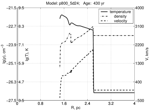
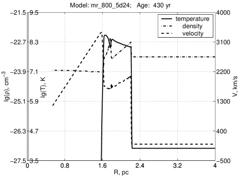
Fig. 1: Temperature (solid), density (dash-dotted) and velocity (dashed) profiles for models: left: WD065; right: MR0

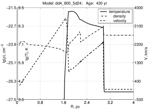
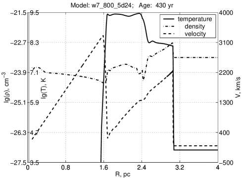
Fig. 2: Temperature (solid), density (dash-dotted) and velocity (dashed) profiles for models: left: DD4; right: W7

Due to different explosion energy in our models, they expand to the given age till different radii, the position of the contact discontinuity (that separates ejecta and ambient medium) for different explosion models also varies from 1.8 to 2.5 pc. Maximum value of the shocked ejecta density can vary in a range of an order of magnitude for different models. The differences in temperature of heated ejecta are of the order of half magnitude for different models. The width of the heated (therefore, emitting) region varies also quite noticeably. All these varieties lead to the differences in the emission one could observe from the remnant.

Results of the spectra simulations for different explosion models are shown in Fig.3 and Fig.4. The gray line corresponds to $N_{H}=4\times 10^{21}\,\mbox{cm}^{-2}$ galaxy column density, the black one – to $N_{H}=9\times 10^{21}\,\mbox{cm}^{-2}$.

These plots show that we can rule out the WD065 model (it shows very weak Fe K–line, contrary to the EPIC observation with XMM–Newton by Decourchelle et al. 2001). All Chandrasekhar-mass models produce almost the same spectra with similar strength of lines. Though Fe K emission is a bit stronger in MR0, it is not possible to judge which of these models is better.

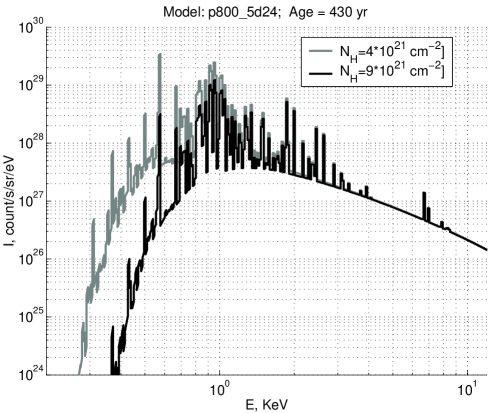
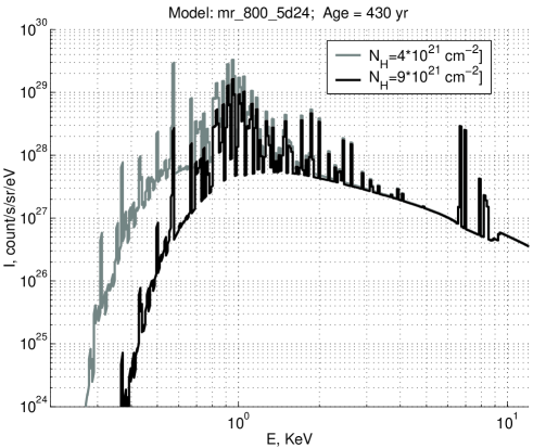
Fig. 3: Full theoretical X-ray spectra (with the account of interstellar absorption for column density $N_{H}$) of the simulated remnant in XMM-Newton range (0.2-10 keV) for various types of models: left: WD065; right: MR0

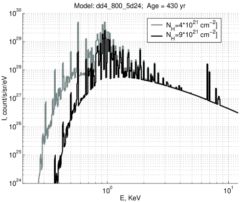
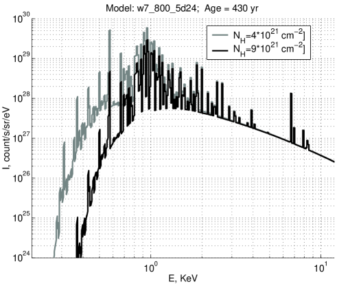
Fig. 4: Full theoretical X-ray spectra (with the account of interstellar absorption for column density $N_{H}$) of the simulated remnant in XMM-Newton range (0.2-10 keV) for various types of models: left: DD4; right: W7.

Much more drastic differences arise when we look at the profiles of the remnant in bandwidths of various ion lines and compare these with observed azimuthally averaged radial profiles of the deconvolved images in various lines (Decourchelle et al. 2001).

We plot (Fig.5 and Fig.6) the profiles of the simulated remnant in different lines (e.g., in FeXVII line and Si K line). Models DD4 and W7 give comparable profiles, but Si and Fe lines are separated strongly in space, WD065 is distinguished strongly from the others and from the observational data, while MR0 shows the best agreement with observations: the diameters of the remnant in Si and Fe lines are very close, an amplitude of the luminosity variations in the corresponding lines is also more similar to what is observed by Decourchelle et al. 2001.

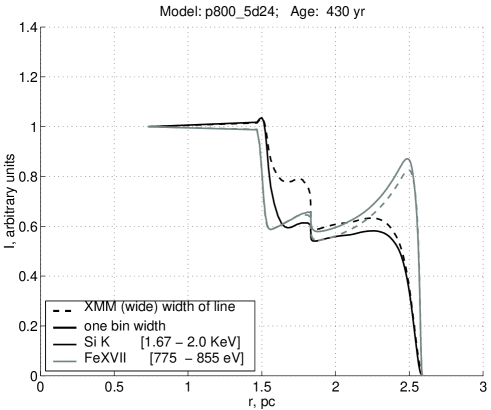
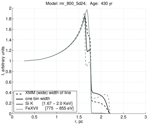
Fig. 5: Profiles of the remnant’s brightness in lines of Si K and FeXVII ions, integrated over line of sight. Dashed line shows a profile of emission within a range 1.67-2.0 keV (Si K) and 775-855 eV (FeXVII). Solid line shows emission within a range of one bin ($\Delta E=13.6$ eV @ 1 keV) that presumably corresponds to the emission line of Si K or FeXVII. Left: WD065; right: MR0

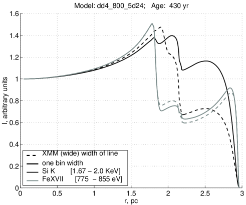
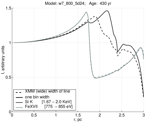
Fig. 6: Profiles of the remnant’s brightness in lines of Si K and FeXVII ions, integrated over line of sight. Dashed line shows a profile of emission within a range 1.67-2.0 keV (Si K) and 775-855 eV (FeXVII). Solid line shows emission within a range of one bin ($\Delta E=13.6$ eV @ 1 keV) that presumably corresponds to the emission line of Si K or FeXVII. left: DD4; right: W7

Discussion and prospects

Though the results are very preliminary, we can rule out the sub-Chandrasekhar-mass model WD065 for the Tycho SNR. The most popular models DD4 and W7 show relatively good agreement with observational data (though the radial profiles are not very encouraging). Nevertheless, the most promising model is still MR0. It fits better both the observed X-ray spectrum and the brightness profiles in different lines.

To make our results more reliable, we still need to upgrade our techniques in order to obtain a better agreement with X-ray observations. There is a number of issues that have to be worked out.

Since we do not know exactly the ionization stage (thus the “true” equation of state) of plasma on the hydro calculation step, we should calculate it by our time-dependent code. But due to our limited computer resources we cannot make it in a fully self-consistent way immediately. Instead, we can calculate separately and save the history of ionization and then perform the second iteration of flow calculation with the new (updated) set of ionization data.

In the modelling we assume $T_{e}=T_{i}$ in the calculations. We can introduce a parameter that specifies relationship between $T_{e}$ and $T_{i}$. Variations of this parameter will affect the spectrum shape. Thus we can find a value of the parameter that will make a best fit to spectrum.

We have only tested CSM with a constant density. In near future we plan to test also “windy” CSM, with density gradient. That will change the dynamical evolution and, probably, the emission of our models.

At last, looking at the spectra one can see, that Decourchelle et al. 2001 show very broad lines and we have them rather narrow, although we have taken into account thermal and Doppler broadening. Convolving our theoretical curves with XMM-Newton response matrix (EPIC, MOS and PN instruments) would give us a possibility for more accurate data fitting.

Taking into account all the above issues we will make the comparison of models and observations more correct and fruitful. Nevertheless, we believe that the main conclusion of this work will remain unchanged: the new 3D SN Ia model MR0, due to its low energetics and a strong mixing, seems the best to model Sn Ia remnants, as well as their light curves.

Acknowledgements. The work is supported in Russia by RFBR grant 02-02-16500.

E-mail address of D.I. Kosenko lisett@xray.sai.msu.ru
Manuscript received 19 October 2002; revised 19 October 2002; accepted 19 October 2002.

References

- [1] Baade W., Astroph. J., 102, 309, 1945.
- [2] Blinnikov, S.I., Bartunov, O.S., Astron. Astrophys., 273, 106, 1993.
- [3] Blinnikov, S.I., Sorokina E.I., Hunting the Cosmologocal Parameters, Eds. D. Barbossa et al., KLUWER, 2003.
- [4] Blinnikov, S.I. et al.; Astroph. J., 532, 1132, 2000.
- [5] Borkowski, K.J., Lyerly, W.J., and Reynolds, S.P., Astroph. J., 548, 820, 2001.
- [6] Brinkmann, W., Fink, H.H., Smith, A., and Haberl, F., Astron. Astrophys., 221, 385, 1989.
- [7] Chevalier R.A., Raymond J.C., Astroph. J. Lett., 225, L27, 1978.
- [8] Davison P.J.N., Culhane J.L., Mitchell R.J., Astroph. J. Lett., 206, L37, 1976.
- [9] Decourchelle A. et al.,Astron. Astrophys., 365, L218, 2001.
- [10] Dickel J.R. et al., Astroph. J., 257, 145, 1982.
- [11] Duin R.M., Strom R.G., Astron. Astrophys., 39, 33, 1975.
- [12] Hamilton A.J.S., Sarazin C.L., Szymkowiak A.E., Astroph. J., 300, 713, 1986.
- [13] Hwang U., Gotthelf E.V., Astroph. J., 475, 665, 1997.
- [14] Hwang U., Hughes J.P., Petre R., Astroph. J., 497, 833, 1998.
- [15] Itoh H., Masai K., Nomoto K., Astroph. J., 334, 279, 1988.
- [16] Nomoto, K., Thielemann, F.K., Yokoi, K., Astroph. J., 286, 644, 1984.
- [17] Reinecke, M., Hillebrandt, W., Niemeyer, J. C., Astron. Astrophys., 386, 936, 2002.
- [18] Ruiz-Lapuente, R. et al., Nature, 365, 728, 1993.
- [19] Seward F., Gorenstein P., Tucker W., Astroph. J., 266, 287, 1983.
- [20] Tsunemi H et al., Astroph. J., 306, 248, 1986.
- [21] van den Bergh S., Astroph. J., 168, 37, 1971.
- [22] van den Bergh S., Marscher A.P., Terzian Y., Astroph. J. Suppl., 26, 19, 1973.
- [23] Vancura O., Gorenstein P., Hughes J.P., Astroph. J., 441, 680, 1995.
- [24] Woosley, S.E., Weaver, T.A., Supernovae, Eds. J. Audouze et al., ELSEVIER, Sci.Pub., Amsterdam, 63, 1994.
- [25]