Energy exchange inside SN ejecta
and light curves of SNe Ia

E.I. Sorokina¹, S.I. Blinnikov<sup>2,1

1</sup> Sternberg Astronomical Institute, Moscow, Russia
² Institute for Theoretical and Experimental Physics, Moscow, Russia

A treatment of line opacity is one of the most crucial problems for the light curve (LC) modeling of Type Ia supernovae (SNe Ia). Spectral lines are the main source of opacity inside SN Ia ejecta from ultraviolet through infrared range. A lot of work has been done on this subject [1, 3, 6, 7, 8, 9].

The problem itself can be divided into two parts:

• How flux and energy equations are changed in the expanding medium;

• How one should average flux and intensity, as well as extinction and absorption coefficients, over energy bins used in calculations.

Almost all previous research was about the flux equation. Here we will focus on the energy equation. We will suppose a free expansion of gas, i.e. linear law for the velocity distribution $v=r/t$. The principal difference between the behavior of flux and intensity in comparison to the static case is that the flux always becomes lower in the expanding media, while the sign of the change of intensity depends on the temperature gradient. It is clear qualitatively. When we are sitting inside the gas and would like to measure a flux and an intensity at a fixed frequency in the static case we should just measure how the surrounding gas emits and absorbs at this frequency. If this specific frequency corresponds to a strong line we will not be able to see distant layers of gas, since rather large optical depth accumulates quite close to the observer. In the continuum we can see rather distant gas layers. So at the frequency of a strong line we observe almost local gas without temperature gradient, hence we measure rather low flux value, and the intensity corresponds to the local blackbody value. In the continuum the flux grows appreciably because of growing gradients, and the intensity corresponds to the blackbody at $\tau\sim 1$, where conditions differ from local ones.

Figure 1: Left panel: the zero moment of an occupation number $f_{0}$. Dots correspond to the local blackbody value, dashes show the blackbody at the distance where continuum forms, solid line demonstrates the behavior of $f_{0}$ when five spectral lines are present in the frequency interval we are interested in. Right panel: logarithms of monochromatic $\alpha$ (thick lines, “top hat” profile), $b-j$, and $\alpha(b-j)$. The main problem is to integrate the last function, especially when the number of lines is not 5, but several hundreds.

In the expanding case, a photon’s mean free path becomes less than in the static medium, even at the frequency which corresponds to the continuum at the rest observer frame. If we encounter a strong line blueward, before $\tau\sim 1$ is reached in continuum, then, most probably, we will not be able to see further out. So the temperature gradient at the mean free path of a photon becomes less than in the static case, therefore the flux drops down. The intensity in the expanding medium would then correspond to the blackbody radiation at the distance where the line forms, but it is redshifted by Doppler effect. For a constant temperature and pure continuum, the intensity at any space point and any frequency is lower than the local blackbody intensity. A strong nearby line enhances the value of the observed intensity (opposite to the behavior of the flux, which drops down with the comparison to a pure continuum case) and diminishes the difference between this intensity and a local blackbody. Fig. 1 shows all these dependencies for the zero moment of an occupation number, which is proportional to an angle averaged intensity (the zero moment of intensity): $J_{\nu}={2h\nu^{3}\over c^{2}}f_{0}$; $J_{\nu}={1\over 2}\int_{-1}^{1}I_{\nu}d\mu$.

To derive these dependencies formally, we have to solve the Boltzmann equation in the comoving frame for a spherically-symmetrical flow:

$${1\over c}{\partial f\over\partial t}+\mu{\partial f\over\partial r}+{1-\mu^{2}\over r}{\partial f\over\partial\mu}-{\nu\over ct}{\partial f\over\partial\nu}=\eta_{\nu}-\chi_{\nu}f\;,$$ (1)

where we put $r=vt$, which is quickly established in SN ejecta. When we apply a diffusion limit, so that the space derivatives are negligible, the solution of the Boltzmann equation is [3]

$$f_{0}=\int_{\nu}^{t\nu/t_{0}}{\nu\over\tilde{\nu}^{2}}\;\alpha^{\star}(t\nu/\tilde{\nu},\tilde{\nu})\,b(t\nu/\tilde{\nu},\tilde{\nu})\exp\left[-\int_{\nu}^{\tilde{\nu}}{\nu\over\bar{\nu}^{2}}\;\alpha^{\star}(t\nu/\bar{\nu},\bar{\nu})\;d\bar{\nu}\right]\;d\tilde{\nu}\;,$$ (2)

where $b$ is a blackbody occupation number, and the dimensionless absorption coefficient $\alpha^{\star}=\alpha ct$.

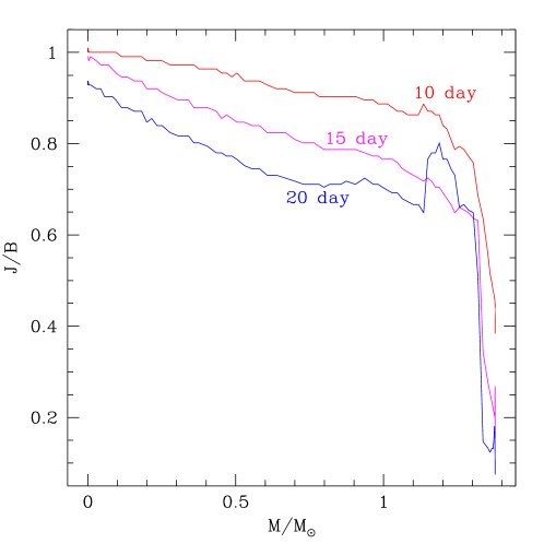
Figure 2: The distribution of $J/B$ inside the ejecta at different times demonstrates how matter and radiation are decoupled.

Last equation gives us an exact solution for a monochromatic value of $f_{0}$. Numerical codes which are used for computations of SNe radiative evolution operate with averaged numbers, and each energy bin contains hundreds of spectral lines. During such computations one needs to solve equations for energy exchange between radiation and gas in each bin:

$${d<j_{\nu}>\over dt}\;\propto\;<\alpha_{\nu}>(<b_{\nu}>-<j_{\nu}>).$$ (3)

The problem here is to average $\alpha$ correctly inside a bin with hundreds (or thousands) of lines. The right way is to average it so that

$$<\alpha>={<\alpha(b-f_{0})>\over<b>-<f_{0}>}\qquad(f_{0}\equiv j_{\nu}).$$ (4)

The main difficulty here is to derive an average value of $<\alpha(b-f_{0})>$. As we said above, in the strong lines $f_{0}=b$. If an optical depth in the continuum is also very high, so that radiation is tightly coupled with matter and $f_{0}=b$, then $b-f_{0}\approx 0$ and it is not so important how we treat $\alpha$. It becomes important when radiation is decoupled from matter. As it is seen in the fig. 2, they are decoupled within the entire SN Ia ejecta even before maximum light (which occurs about 20th day after explosion). A similar result was obtained in [5]. So the correct treatment of $<\alpha>$ is essential. We need to take the integral (2) accurately. It is very hard to do numerically, since $\alpha$ jumps up and down by many orders of magnitude hundreds of times. Moreover, where $\alpha$ is high, there $b-f_{0}$ is extremely small (see fig. 1). Analytically, one can solve this problem, but only for very simple line profiles. We assume that lines have a rectangle shape (“top hat” profile). For rectangle lines in the Rayleigh–Jeans regime and infinite expanding medium (so that at given $\nu$ one can observe emission with arbitrary shifted $\Delta\nu$ in the transparent case) we have

$$f_{0}(\nu)={kT\over h\nu}\Biggl{[}\!\!\Biggl{[}1-{1\over\alpha^{\star}_{N_{\nu}}}\left(1-e^{-\alpha^{\star}_{N_{\nu}}(1-{\nu\over\nu_{N_{\nu}}})}\right)\qquad\qquad\qquad\qquad\qquad\qquad\qquad\qquad$$

$$-\sum_{j=N_{\nu}+1}^{N_{\rm max}}\left[{1\over\alpha^{\star}_{j}}\left(1-e^{-\alpha^{\star}_{j}({\nu\over\nu_{j-1}}-{\nu\over\nu_{j}})}\right)\exp\left\{-\sum_{i=N_{\nu}}^{j-1}\alpha^{\star}_{i}\left({\nu\over\nu_{i-1}}-{\nu\over\nu_{i}}\right)\right\}\right]\qquad$$

$${}-{1\over\alpha^{\star}_{N_{\rm max}+1}}\left(1-e^{-\alpha^{\star}_{N_{\rm max}+1}\nu/\nu_{N_{\rm max}}}\right)\exp\left\{-\sum_{i=N_{\nu}}^{N_{\rm max}}\alpha^{\star}_{i}\left({\nu\over\nu_{i-1}}-{\nu\over\nu_{i}}\right)\right\}\Biggr{]}\!\!\Biggr{]}$$ (5)

To get $<\alpha>$ from (4), we need to integrate this expression once more. This also can be done analytically, and adds the third summation over all lines in the bin. Computing of these long sums is very time consuming. Probably, the efficiency can be improved along the way proposed in [2].

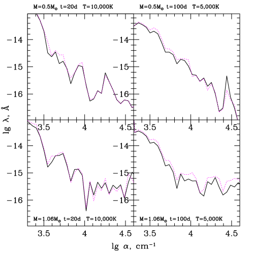
Figure 3: Logarithm of absorption coefficient calculated accordingly to our formulae (solid) and in Eastman–Pinto approximation (dotted). Top panels show the absorption for two sets of (time, temperature) inside the layer of W7 model which consists of mostly ⁵⁶Ni, while bottom panels correspond to the layer of intermediate mass elements.

Using our expression for $<\alpha>$, we have computed the opacity tables for standard SN Ia model W7. The results are compared with the absorption derived with the Eastman–Pinto approximation [7] (see fig. 3). In the UV region, where free–free and bound–free emission dominates, $<\alpha>$ remains almost unchanged, while it differs up to a factor of two in the range between near UV through IR.

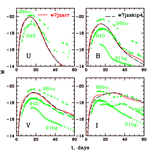
Figure 4: UBVI light curves of the model W7 with two opacity approximations: Eastman–Pinto (black dashed) and the way of averaging presented here (red solid). UBV bands remain almost unaffected, while I–band shows now a complicated structure, more similar to what one can observe for real SNe Ia, though not identical. Crosses, stars and triangles show the observational LCs for three SNe Ia.

LCs for W7 (fig. 4) were calculated with the help of the code STELLA [4]. UBV LCs remain almost unchanged, while I-band is affected appreciably (fig. 4). This is explained by the changes of opacity and spectrum in the I-band.

Acknowledgements

We are grateful to the organizers of the Ringberg meeting for their hospitality, to Stan Woosley for supporting our work in the UCSC. Our work in US was supported by grants NSF AST-97 31569 and NASA - NAG5-8128, in Russia RBRF 99-02-16205 and RBRF 02-02-16500.

References

- [1] E. Baron, P.H. Hauschildt, A. Mezzacappa, MNRAS 278 (1996) 763.
- [2] B. Baschek, W. v. Waldenfels, R. Wehrse, A&A 371 (2001) 1084.
- [3] S.I. Blinnikov, Astron.Lett. 22 (1996) 79.
- [4] S.I. Blinnikov et al., ApJ 496 (1998) 454.
- [5] R.G. Eastman, in Thermonuclear Supernovae. Eds. P. Ruis-Lapuente et al. – Dordrecht: Kluwer Academic Pub., (1997) p. 571.
- [6] R.G. Eastman and R.P. Kirshner, ApJ 347 (1989) 771.
- [7] R.G. Eastman, P.A. Pinto, ApJ 412 (1993) 731.
- [8] A.H. Karp et al., ApJ 214 (1977) 161.
- [9] R.V. Wagoner, C.A. Perez, M. Vasu, ApJ 377 (1991) 639.