Limits on Galactic Dark Matter
with 5 Years of EROS SMC Data

Five years of  data towards the Small Magellanic Cloud have been searched for gravitational microlensing events, using a new, more accurate method to assess the impact of stellar blending on the efficiency. Four long-duration candidates have been found which, if they are microlensing events, hint at a non-halo population of lenses. Combined with results from other  observation programs, this analysis yields strong limits on the amount of Galactic dark matter made of compact objects. Less than 25% of a standard halo can be composed of objects with a mass between $2\times 10^{-7}\,\rm M_{\odot}$ and 1 $\rm M_{\odot}$ at the 95% C.L.

1 Research context

The idea of using gravitational microlensing as a tool to probe the dark matter in the Galactic halo goes back to 1986 with a paper by B. Paczyński (Paczyński,, 1986). Since then, several experiments have been monitoring millions of stars towards the Large and Small Magellanic Clouds (lmc and smc) and candidates have been observed towards the two targets (Alcock et al.,, 1993; Aubourg et al.,, 1993; Ansari et al.,, 1996; Alcock et al., 1997a, ; Afonso et al.,, 1999; Lasserre et al.,, 2000).

The detection of candidates towards the lmc suggested a population of lenses accounting for $\sim$20% of a standard halo, with a most probable mass between 0.2 and 0.9 M_⊙ (Alcock et al.,, 2000). Results by Lasserre et al., (2000) show that objects up to 1 M_⊙ cannot account for more than 40% of a standard halo. These lenses cannot be ordinary Galactic stars, whose density is much too low to account for the observed optical depth, and Goldman et al., (2002) demonstrated they cannot be halo white dwarfs with hydrogen atmosphere. Much debate has occurred on the nature and the location of the lenses, the main two possibilities being 0.4 M_⊙ dark objects in the halo or stars at the low mass end of the main sequence in the clouds themselves (Sahu,, 1994; Wu,, 1994).

This makes the smc a very valuable target. While the characteristics (optical depth and duration) of events towards the two clouds should be similar for halo lenses (Sackett and Gould,, 1993), the different dynamical properties of the clouds could account for differences if the events are due to self-lensing.

The eros 2 experiment has been surveying the smc since 1996. We present here an analysis of five years of data accumulated towards this target.

2 Experimental setup and SMC observations

The telescope, camera, telescope operations and data reduction are as described in Palanque-Delabrouille et al., (1998), hereafter sm98, and references therein. Since July 1996, 10 one-square-degree fields have been monitored towards the smc. The first 5 years of data from 8.6 square degrees spread over these 10 fields have been analyzed. The data set contains about 5.2 million pairs of light curves in two wide pass bands called thereafter “red” and “blue”, sampled on average once every 2.5 days from end-April to mid-March when the smc is visible. About 400–500 images of each field were taken, with exposure times ranging from 5 minutes in the center of the smc to 15 minutes in the outermost region.

3 Data analysis

The analysis of the five-year data set is similar to those of the first year (sm98) and of the first two years (Afonso et al.,, 1999) of data where details can be found.

A first set of cuts is designed to select light curves that exhibit a single significant fluctuation. This already excludes 99.8% of the stars, most of which exhibit flat light curves.

A second set of cuts rejects stars that are a priori likely to be variable, based upon their position in a color-magnitude diagram: bright blue stars in the upper main sequence with low-amplitude variations and stars much brighter and redder than those of the red clump are rejected. These stars are contained in two thinly populated regions of the color-magnitude diagram, so rejecting them does not reduce much the number of light curves on which we can search for microlensing. Stars exhibiting a strong correlation between the red and the blue light curves outside the period containing the main fluctuation are also rejected. Supernovae are rejected by the comparison of the rising and falling times of the variation. Half of the light curves surviving the first set of cuts are rejected at this stage, leaving about 5000 light curves.

A third set of cuts improves the signal-to-noise ratio of the set of selected candidates by comparing the measurements with the best-fit point-source point-lens microlensing light curve. These criteria are sufficiently loose not to reject light curves affected by blending, parallax and most cases of binary lenses or sources. The remaining sample consists of about 30 light curves exhibiting a clean and unique fluctuation with a smooth time variation.

A fourth set of cuts constrains the time coverage of the event, excluding in particular all events with Einstein radius crossing times $t_{\rm E}$ exceeding 1200 days.

The final criterion is as follows: if blending significantly improves the fit, then the fitted blending should be physical, i.e. indeed correspond to the amplification of only a fraction of the total flux recovered.

To limit contamination of the set of selected candidates by spurious events, the levels of the above cuts are set such that most variable stars are rejected by at least two of them. The tuning of each cut and the estimation of the efficiency of the analysis is done with Monte Carlo simulated light curves, as described in sm98. Microlensing parameters are drawn uniformly in the following intervals: time of maximum magnification $t_{0}$ within the observing period $\pm 300$ days, impact parameter normalized to the Einstein radius $u_{0}\in[0,1.5]$ and time-scale $t_{\rm E}\in[0,1200]$ days.

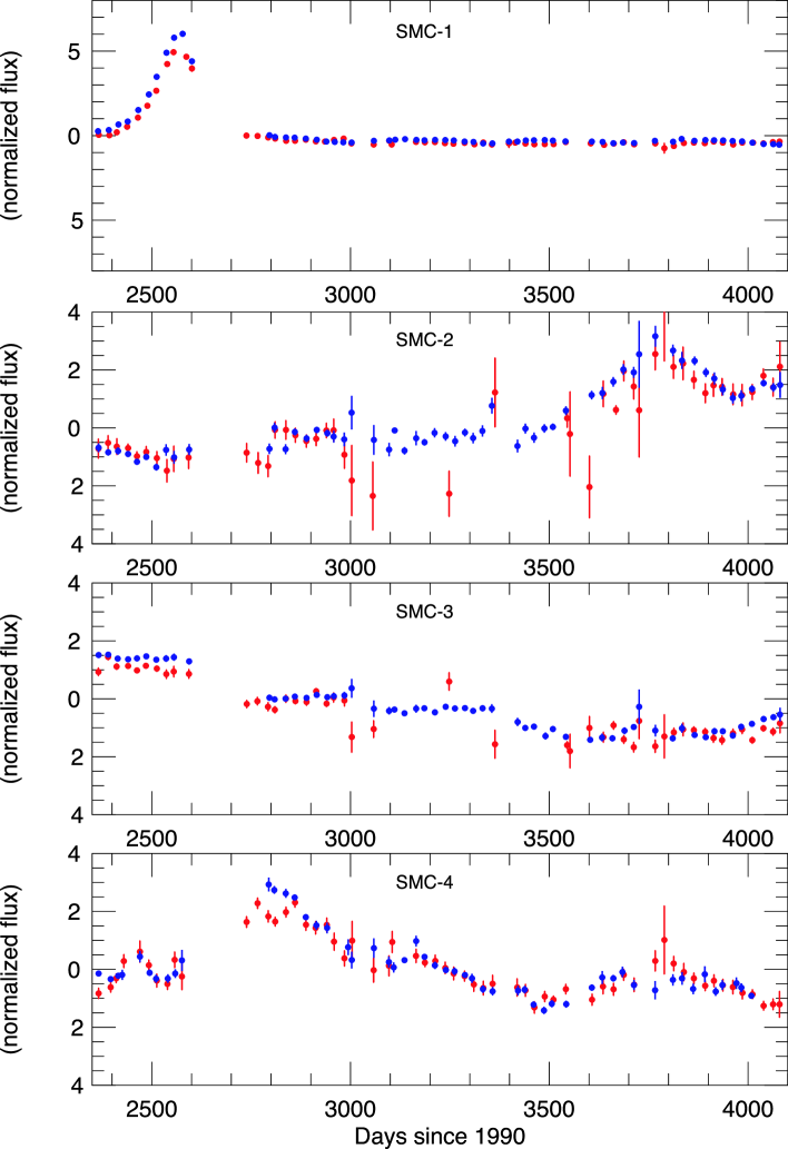
Four candidates (smc-1 to smc-4) pass all the cuts. Their light curves are shown in figure 1, their coordinates are given in table 1 and the microlensing fit parameters (point-source, point-lens and no-blending) in table 2.

Figure 1: Red light curves of the microlensing candidates detected towards the smc.

Table 1: Coordinates (J2000) and baseline photometry of the candidates.

	$\alpha$	$\delta$	$V_{J}$	$I_{C}$
smc-1	01:00:05.73	-72:15:02.33	17.9	17.9
smc-2	00:48:20.16	-74:12:35.31	20.4	19.5
smc-3	00:49:38.68	-74:14:06.77	20.2	19.3
smc-4	01:05:36.56	-72:15:02.39	19.9	19.4

Table 2: Results of microlensing fits to the smc candidates. $u_{0}$ is the impact parameter and $t_{\rm E}$ the Einstein radius crossing time in days.

	$u_{0}$	$t_{\rm E}$	$\chi^{2}/{\rm d.o.f.}$
smc-1	0.52	101	1026/706
smc-2	0.82	390	1526/990
smc-3	0.66	612	2316/968
smc-4	0.80	243	2923/951

Candidate smc-1 is the one already present in the previous analyses (one year and two years of smc data) done by eros. Further analysis of its light curve indicated that it was probably a self-lensing event (sm98). It was also detected as a possible microlensing candidate by the online trigger system of the macho experiment (Alcock et al., 1997b, ). Candidates smc-2, smc-3 and smc-4 have very long durations, with few points outside the amplified region of the light curve. The $\chi^{2}/{\rm d.o.f.}$ of candidate smc-4 is large, yet far from the cut level (which is set at 5.0 in the peak region). All three candidates, however, exhibit features in their baseline that are reminiscent of variable stars. These features appear clearly on the light curves plotted in 25-day bins (see figure 2). To allow a direct comparison of the red and blue fluxes, all fluxes have been normalized so that they would have a mean of zero and a variance of unity. Candidates smc-2 and smc-4 clearly look like irregular variables, while smc-3 has an irregular light curve and seems to be rising at the end. These candidates will need to be monitored for several more years to be either confirmed but most probably ruled out as microlensing candidates. They are not in the $\sim$3 square degrees of the smc on which the macho project took data.

Figure 2: Red and blue light curves of the microlensing candidates detected towards the smc, in 25-day bins.

The efficiency of the analysis for events with (Monte-Carlo) $u_{0}<1.5$ normalized to an observing period $T_{\rm obs}$ of five years is summarized in table 3.

Table 3: Detection efficiency $\epsilon$ in % as a function of the timescale $t_{\rm E}$ in days for events with $u_{0}<1.5$ and normalized to $T_{\rm obs}=5{\rm\>yr}$.

$t_{\rm E}$	5	15	50	125	325	500	900	1100	1300
$\epsilon$	2.1	6.3	11.1	13.8	11.8	10.1	7.5	5.9	2.7

4 Blending effect

The above efficiencies have been derived without taking account of stellar blending.

We have performed a study to quantify precisely the influence of blending on our results. We simulate an experiment with synthetic images, regularly spaced in time, in which microlensing events are embedded. The images are built from the hst colour-magnitude diagram (CMD) and luminosity function (LF) of the Magellanic Clouds, which extend well beyond the eros detection limit (down to V=23.5 in the hst data). We have checked that the CMD and LF that we construct from these simulated images are in good agreement with those obtained from our data. All stars are lensed for a timescale $t_{\rm E}$ of 5 images. The impact parameter $u_{0}$ is drawn uniformly between 0 and 1.5, and $t_{0}$ is set so that no two stars less than 20 pixels apart are magnified simultaneously (typical eros images have a seeing of 2.1 arcsec corresponding to a gaussian with rms of 1.5 pixel).

The standard photometry chain of eros is applied to these images, leading to the detection of 5599 objects (in this terminology an object usually encompasses several simulated stars) with their red and blue light curves. A total of 6304 generated microlensing events were found with $u_{0}<1$ and an average timescale $\langle t_{\rm E}\rangle=3.16$ images. The effect of blending is readily seen from the fact that more events than objects are detected. Of these events, 60% are due to the brightest star in the two pixels around the object, with recovered $\langle t_{\rm E}\rangle=4.00$ images and $\langle u_{0}\rangle=0.52$, close to the generated values. The remaining events are due to a fainter, blended component of the object, with recovered $\langle t_{\rm E}\rangle=1.89$ images, well underestimated, and $\langle u_{0}\rangle=0.64$, clearly overestimated, as expected from the impact of a significant blend. The optical depth being proportional to the number of events and to their mean $t_{\rm E}$, an estimate of the ratio $R$ of the recovered optical depth to the generated one is:

$$R=\frac{6304}{5599/1.5}\frac{3.16}{5.0}=1.07\;,$$

with an estimated error of about 10%.

The light curves from the above blending simulation are then used as templates in our Monte Carlo chain designed to compute the efficiency of our analysis (section 3) as follows: for each object detected in the actual data, an object is randomly chosen from the blending simulation in the same region of the CMD. The light curve of the latter is shifted and stretched to account for the randomly selected duration and time of maximum amplification, but the amplitudes in each colour are of course kept as found in the blending simulation to reflect the impact of the underlying stellar companions of the microlensed star. This template is used (instead of the standard shape derived by Paczyński in the absence of blending and used for the efficiency computation in the previous section) to add a microlensing event to the real (flat in most cases) light curve. To ensure similar photometric dispersion in the Monte Carlo and in the data, the rms flux deviation of each simulated data point from the blended microlensing light curve is taken to be the same as the deviation of the real light curve from constant brightness. The modified light curve goes through the same analysis cuts as in the standard computation of the efficiency.

The efficiency with the blending simulation described above is within 10% of the efficiency computed from the standard procedure, in agreement with estimates in previous works (Palanque-Delabrouille,, 1997). The loss due to the under-estimation of the magnification of a blended event (the observed magnification on a blended object is lower than the physical magnification of the underlying star) is almost exactly compensated by the fact that an object includes more than one star subject to lensing. In addition, as expected, the cuts of the analysis are sufficiently loose not to reject blended microlensing events. In particular, there are no cuts requiring a strict achromaticity of the event. For the eros experiment, blending has a small impact on the efficiency and can therefore be neglected.

5 Limits

In order to set limits on the contribution of dark objects to the halo, we use the so-called “standard” halo model described in sm98 as model 1, and take into account the efficiency of the analysis given in section 3.

For a given experiment, assuming that the halo is made of compact objects having a single mass $M$, we define $P_{M}(t_{\rm E})$ as the probability distribution of expected event durations, taking efficiencies into account, and $f\tilde{N}_{\negthinspace M}$ as the expected number of events, where $f$ is the halo mass fraction with respect to a full standard halo. We construct a frequentist confidence level $1-p_{n}$ considering only the number $n$ of observed events as a Poisson process:

$$1-p_{n}=\sum_{i=0}^{n}\frac{e^{-f\tilde{N}_{\negthinspace M}}(f\tilde{N}_{\negthinspace M})^{i}}{i!}$$

We also make an independant Kolmogorov test comparing the observed event durations to the expected $P_{M}(t_{\rm E})$ distribution, and obtain a Kolmogorov probability $p_{t}$.

A well known prescription for the confidence level of the combined test is

$$p=p_{n}p_{t}(1-\ln p_{n}p_{t})$$

Our experiment has however an unknown contribution of background — variable stars or any other unknown phenomenon — to the observed candidates. We therefore test all combinations, attributing candidates either to signal or background, and retain, for every mass fraction $f$, the configuration that maximizes $p$, i.e. the most conservative one. This ensures that we have a given frequentist coverage for all possible hypotheses.

We then set a frequentist 95% CL limit on $f$, taking into account both the number of candidates and their duration, by finding the value of $f$ that yields $p_{max}=0.05$.

Although this prescription could be used to combine several experiments, it gives the same weight to all and does not yield useful results if the sensitivities of some of the experiments differ significantly. Therefore, to combine various experiments, we use instead a Liptak-Stouffer (Liptak,, 1958) prescription where the flat p-values are converted to unit-variance, zero-mean gaussian distributed variables. A weighted sum of these variables is also gaussian distributed, and can be converted back to a p-value. We take as weights the expected number of events of each experiment for each lens mass.

The results obtained by the various phases of eros (which are independent experiments) are summarized in table 2 for microlensing candidates towards the smc — no smc candidate in eros1 (Renault et al.,, 1998), 4 candidates in eros2 (sm98 and present work) — and in table 4 for microlensing candidates towards the lmc — no planetary mass candidate (Renault et al.,, 1997, 1998), lmc-1 from eros1 photographic plates (Ansari et al.,, 1996) and the others from eros2 (Lasserre et al.,, 2000; Lasserre,, 2000; Milsztajn et al,, 2001).

Table 4: Summary of the microlensing candidates detected by eros towards the lmc. The parameters are the same as in table 2.

	$u_{0}$	$t_{\rm E}$
lmc-1	0.44	23
lmc-3	0.21	44
lmc-5	0.59	24
lmc-6	0.41	35
lmc-7	0.30	30

Figure 3 shows the 95 % exclusion limit derived from this method on $f$, the halo mass fraction, at any given mass $M$ — i.e. assuming all deflectors in the halo have mass $M$ — for the eros1 ccd lmc and eros1 ccd smc, eros1 photographic plates, eros2 3-year lmc and eros2 5-year smc experiments, and for the combination of all. We also show in the figure the limits that would be obtained with a single smc event (smc-1), then with no event at all in any of the eros experiments, which indicates the overall sensibility of the eros project, considering presently analysed data.

Figure 3: Exclusion diagram at 95 % C.L. for the standard halo model ($4\times 10^{11}\>{\rm M}_{\odot}$ inside 50 kpc). The dashed lines are the limits towards the lmc by eros 1 and eros 2, the thin plain lines are limits towards the smc  and the thick line is the combined limit from the five eros sub-experiments. The dotted lines are the limits that would be obtained considering no observed events: they indicate the overall sensibility of the eros dataset. We also indicate the limit that would be obtained if the three very long duration events on the smc were considered as background (label “smc-1 only”) : the limit is lowered in a negligible way in the 2–3 $\rm M_{\odot}$ mass range.

The “dent” in the eros1 plate limit and in the eros2 lmc limit at a mass near $0.5\rm M_{\odot}$ is the impact of the $\sim$30 day candidates observed towards the lmc. For any mass between $2\times 10^{-7}$ and $10^{-1}\leavevmode\nobreak\ {\rm M}_{\odot}$, we exclude at 95 % C.L. that more than 20% of the mass of a standard halo be made of compact objects. It can be seen that the combined limit is above the best limit for some values of the mass. This occurs quite naturally since the observed smc and lmc candidates have quite different characteristics. At high mass, for instance, our method will consider smc candidates as signal and lmc candidates as background, thus weakening the limit obtained by the lmc alone. It illustrates the (marginally significant) incompatibility between the candidates observed by eros towards the smc and the lmc.

6 Comparison of LMC and SMC results

Another way to gauge the present results on microlensing towards the smc is to compare them directly to the result of the macho collaboration towards the lmc (Alcock et al.,, 2000). Such a comparison is made easier by the fact that the expected $t_{E}$ distributions of halo microlenses towards the smc and lmc are very similar: their averages and widths differ by only a few percent, and these differences are much smaller than the widths themselves. The ratio of the optical depths towards the smc and lmc is more uncertain; for a spherical isothermal halo, it is expected to be about $\tau_{SMC}/\tau_{LMC}\simeq 1.4$, but this value can be lower for flattened halos. Actually, it was proposed to use observations towards the smc to evaluate the galactic dark halo flattening (Sackett and Gould,, 1993).

In their analysis A, the macho group has listed 13 microlens candidates with an average duration $<t_{E}>\,=36$ days and a width of the $t_{E}$ distribution compatible with all microlenses having the same mass. From this, they compute an optical depth $\tau=1.2\times 10^{-7}$, of which about $1.0\times 10^{-7}$ is attributed to halo lenses. This translates into an expected number of events for the present eros smc data set of

$$N_{evts}=N_{*}\frac{T_{obs}}{<t_{E}>}\frac{2}{\pi}<\epsilon>\tau_{SMC}\,,$$

where $N_{*}=5.2\,10^{6}$ is the number of smc stars monitored by eros, $T_{obs}=5$ yrs is the total duration of the observations, and $<\epsilon>=0.146$ is the average eros detection efficiency for microlensing events of duration $<t_{E}>\simeq\,0.1$ yr. (This average efficiency is obtained by interpolating the values in Table 3, and is normalized to $u_{0}<1$.) Substituting these numerical values leads to $N_{evts}=2.4\times(\tau_{\rm SMC}/10^{-7})$.

There are, however, no eros smc microlensing candidates that are compatible with the $t_{E}$ distribution observed by the macho group towards the lmc: candidate smc-1, the shortest of all, is very likely due to a lens in the smc (see parallax analysis and the discussion that follows in sm98); the other 3 candidates all have durations longer than 240 days, clearly incompatible with an average of 36 days. From this absence of microlensing candidates with the required duration, eros can exclude $\tau_{SMC}>10^{-7}$ for events similar to those in macho sample A, at better than 90% C.L. The value corresponding to the spherical isothermal halo model, $\tau_{SMC}=1.4\times\tau_{LMC}\simeq 1.4\times 10^{-7}$ is excluded at better than 96% C.L.

7 Discussion and conclusions

The analysis of five years of microlensing data towards the smc yielded four candidates, and allowed to put stringent limits on the amount of galactic dark matter made of compact objects. Objects with a mass between $2\times 10^{-7}\,\rm M_{\odot}$ and 1 $\rm M_{\odot}$ cannot account for more than 25% of the mass of a standard spherical, isothermal and isotropic Galactic halo of $4\times 10^{11}\,\rm M_{\odot}$ out to 50 kpc.

The new method described in this paper to combine the results and use all the information available on the events has one drawback compared to methods used in previous works: it could be more sensitive to the halo model, adding an extra dependence on the velocity distribution. Previously, only the influence of the halo model on the number of expected events has been studied, as in sm98. A change in the velocity distribution, however, would mainly shift the “dent” in the eros2 lmc limit. In addition, since the final exclusion limit is quite flat over a large range of masses, the final result should not be influenced by reasonable changes in the velocity distribution assumptions.

This limit excludes a sizeable fraction of the allowed domain shown in Fig. 12 of Alcock et al. (2000).

All the candidates that have been detected so far towards the smc have long durations, and seem more compatible with unidentified variable stars or self-lensing within the cloud than with halo objects. These would need to have supersolar masses to account for such durations.

The statistics are still very low for a quantitative comparison of the smc and lmc samples of microlensing candidates. They have, however, quite different characteristics which is poorly compatible with a unique population of lenses.