A 6.3-h superhump in the cataclysmic variable TV Columbae: the longest yet seen

Abstract

We present results from a two week multi-longitude photometric campaign on TV Col held in 2001 January. The data confirm the presence of a permanent positive superhump found in re-examination of extensive archive photometric data of TV Col. The 6.3-h period is 15 per cent longer than the orbital period and obeys the well known relation between superhump period excess and binary period. At 5.5-h, TV Col has an orbital period longer than any known superhumping cataclysmic variable and, therefore, a mass ratio which might be outside the range at which superhumps can occur according to the current theory. We suggest several solutions for this problem.

1 Introduction

1.1 Permanent superhumps

Patterson & Richman (1991) initially suggested the term ‘permanent superhump’ for the subclass of cataclysmic variables (CVs) having quasi-periodicities slightly different from their binary orbital periods. Unlike SU UMa systems (see Warner 1995 for a review of SU UMa systems and CVs in general), which show this behaviour only during superoutbursts, permanent superhump systems show the phenomenon during their normal brightness state. However, their amplitudes are highly variable and are sometimes below the detection limits, so the term ‘permanent superhump’ is somewhat misleading.

Whitehurst & King (1991) suggested that superhumps occur when the accretion disc extends beyond the 3:1 resonance radius. According to Osaki (1996), permanent superhumpers differ from other subclasses of non-magnetic CVs in having relatively short orbital periods and high mass-transfer rates, resulting in accretion discs that are thermally stable but tidally unstable. Retter & Naylor (2000) provided observational support for this idea.

The ‘positive superhump’, a periodicity that is a few per cent larger than the orbital period, is explained as the beat period between the binary motion and the precession of an eccentric accretion disc in the apsidal plane. Periods slightly shorter than the orbital periods have also been seen in several systems. They are known as ‘negative superhumps’, and may be generated by the nodal precession of the accretion disc (Patterson et al. 1993; Patterson 1999). However, there are some theoretical difficulties with this idea (Murray & Armitage 1998; Wood, Montgomery & Simpson 2000; Murray et al. 2002). Superhumps were also associated with the formation of a spiral structure in the accretion disc (Steeghs, Harlaftis & Horne 1997; Baba et al. 2002).

Observations of positive superhumps have shown a roughly linear relationship between the period excess, expressed as a fraction of the binary period, and the binary period itself (Stolz & Schoembs 1984). Negative superhumps seem to obey a similar rule (Patterson 1999).

Table 1: Photometric observations of TV Col

Set	Month/year	Nights	Site	Telescope size	Detector	Filter/s	Exposures	Mean night	Number of
				[m]			[s]	length [h]	outbursts
1	12/1985	6	ESO	0.91	photometer	V,B,L,U,W	16	4.2 (gaps)	0
2	12/1985–1/1986	13	SA	0.75+1.0	photometer	white	2	3.0	0
3	11–12/1987	16	ESO	0.91	photometer	V,B,L,U,W	16	5.4 (gaps)	3
4	12/1987	9	ESO	0.91	photometer	V,B,L,U,W	16	5.0	0
5	11/1988	7	ESO	0.91	photometer	V,B,L,U,W	16	4.4 (gap)	0
6	1/1989	6	SA	1.0	CCD	white	40	7.3	0
7	1/1991	9	SA	0.75	photometer	B,R	4	4.8	0
8	12/1991	11	SA	0.75	photometer	white	10	4.0	1
9	1/2001	5	SA+AU+NZ	0.75+0.40+0.25	CCD	white	20-90	11.8	0
10	1/2001	8	SA+AU+NZ	0.75+0.40+0.25	CCD	white	20-90	10.6	0

1.2 TV Col

TV Col is a 14th mag CV at a distance of about 370 pc (McArthur et al. 2001). Its light curve shows multiple periodicities that have attracted many observers. Motch (1981) found periodicities of 5.2 h and 4 d from photometry taken over 10 nights. A radial velocity study by Hutchings et al. (1981) confirmed these periods and detected another at 5.5 h, which they identified as the orbital period. They also pointed out that the 4-d period is exactly the beat periodicity between the other two periods. The 5.2-h period was interpreted as the spin period of a magnetic white dwarf, leading to a classification of the object as an intermediate polar (for reviews of intermediate polars, see Patterson 1994; Warner 1996; Hellier 1996). The detection of a 32-m period in x-ray observations (Schrijver et al. 1985; Schrijver, Brinkman & van der Woerd 1987) confirmed the intermediate polar nature of TV Col, but left the 5.2-h period unidentified.

Further observations confirmed the presence of the three periods in the optical regime (Barrett, O’Donoghue & Warner 1988; Hellier, Mason & Mittaz 1991; Hellier 1993; Augusteijn et al. 1994). The orbital period was also detected in the ultraviolet (Bonnet-Bidaud, Motch & Mouchet 1985). It was found that the 5.2-h period is not stable (e.g. Augusteijn et al. 1994), suggesting that it is a superhump period. The fact that it is shorter than the binary period would make it a negative superhump. Barrett et al. (1988), however, discussed other possible models for the system.

1.3 The significance of superhumps in TV Col

Superhumps have only been observed in CVs with orbital periods below about 3.7 h. Since the orbital period of TV Col is 5.5 h, the interpretation of its 5.2-h period as a negative superhump would make this system an extreme case. There is known to be a strong correlation in CVs between the orbital period and the mass of the secondary star (Smith & Dhillon 1998), which arises because systems with longer orbital periods have larger separations and thus require more massive secondaries to fill their Roche-lobes. The 5.5-h orbital period of TV Col implies a secondary star of $\sim 0.6M_{\odot}$ – much more massive than in other superhumping systems. A typical white dwarf in CVs has a mass of $\sim 1.0M_{\odot}$, which means the mass ratio, $q=M_{\rm donor}/M_{\rm compact}$, in TV Col could be about 0.6 or even higher. This value significantly exceeds the theoretical limit for superhumps – $q\la$0.33 (Whitehurst 1988; Whitehurst & King 1991; Murray 2000). TV Col thus offers a unique opportunity to test the predictions of the models for precessing accretion discs.

There seems to be a strong connection between positive and negative superhumps. Light curves of many permanent superhumpers show both types of superhumps (Patterson 1999; Arenas et al. 2000; Retter et al. 2002). In addition, period deficits in negative superhumps are about half the period excesses in positive superhumps (Patterson 1999): $\epsilon_{\rm negative}\approx-0.5\epsilon_{\rm positive}$, where $\epsilon=(P_{\rm superhump}-P_{\rm orbital})/P_{\rm orbital}$.

This prompted us to examine available photometry of TV Col for positive superhumps, which would be predicted to have a period near 6.3 h. We indeed found such evidence (Retter & Hellier 2000; Retter et al. 2001), which is presented here. At the request of a referee, we then obtained new multi-site photometry on TV Col in 2001 January, which confirmed the 6.3-h period.

2 Photometric data

2.1 Published observations

We have re-analysed existing optical photometry that was presented by Barrett et al. (1988); Hellier et al. (1991); Hellier (1993); Hellier & Buckley (1993) and Augusteijn et al. (1994). This data set contains 77 nights of observations obtained during 1985–1991 over eight separate runs, using the 0.75-m and 1-m telescopes at the South African Astronomical Observatory (SAAO) and the Dutch telescope at the European Southern Observatory (ESO). The main properties of these data are summarized in the first eight rows of Table 1.

2.2 New observations

In 2001 January 2–15 we obtained optical photometry of TV Col from three locations: Sutherland, South Africa (SA) using the 0.75-m telescope with the UCT CCD photometer; Mt Tarana Observatory, Australia (AU; 0.40-m telescope; ST8 CCD) and Auckland, New Zealand (NZ; 0.25-m telescope; ST6 CCD). No filters were used and typical exposure times were a few tens of seconds. Altogether, more than 150 hours of useful data were collected.

For the SA data, PSF-fitting photometry was carried out using a comparison star $9^{\prime\prime}$ NW of TV Col. Aperture photometry yielded similar results, with differences typically less than 0.02 mag. The data from AU and NZ were reduced using aperture photometry, with GSC7059:486 (AU) and GSC7059:754 (NZ) as reference stars. Since different comparison stars were used at the three sites, a linear fit was subtracted from each whole data set before combining them.

Table 2 shows the log of the observations, while Figs. 1 and 2 show the resulting light curve. We see that an outburst of $\sim$1 mag occurred on 2001 January 7, which lasted between 7.6 and 30 h. These data were excluded from the analysis, and the remainder were divided into two sets: before the outburst (Set 9), and afterwards (Set 10). The properties of these sets are included as the last two rows in Table 1.

Figure 1: Light curve of the 2001 January observations (‘clear filter’). A mini-outburst occurred at day 6 of the run.

Table 2: New photometric observations

UT	Time of Start	Run Time	Points	Site	Notes
Date	[HJD]	[h]	number
020101	2451911.895	6.5	541	NZ
020101	2451911.963	3.5	30	AU
020101	2451912.298	7.6	796	SA
030101	2451913.382	5.6	612	SA
040101	2451913.879	6.9	557	NZ
040101	2451913.930	6.6	77	AU
040101	2451914.299	7.6	680	SA
050101	2451915.292	7.7	583	SA
060101	2451915.869	5.5	456	NZ
060101	2451916.291	7.5	774	SA
070101	2451917.287	7.6	650	SA	outburst
080101	2451917.864	4.2	150	NZ
080101	2451918.286	6.5	558	SA
090101	2451919.281	7.4	630	SA
100101	2451920.296	7.2	225	SA
110101	2451920.924	7.4	69	AU
110101	2451921.278	7.6	726	SA
120101	2451922.278	4.3	308	SA
130101	2451922.986	5.7	65	AU
130101	2451923.287	7.0	136	SA
140101	2451923.860	3.2	235	NZ
140101	2451923.986	7.3	85	AU
140101	2451924.277	7.2	678	SA
150101	2451925.276	7.1	756	SA

Figure 2: Light curve of the 2001 January observations (‘clear filter’). Single nights from the three sites are plotted vertically. An offset of 1 mag was imposed between successive nights

3 Analysis

3.1 General remarks

When searching for a 6-h superhump period in the light curve of a variable star there are several complications. Firstly, CVs tend to have night-to-night secular variations of a few tenths of a magnitude that are not related to the periodicity (e.g., Retter, Leibowitz & Naylor 1999). Therefore, very often the best detrending of the data for periodogram analysis is the subtraction of the nightly means / trends. Removing the mean or trends eliminates noise in the power spectrum from this effect. Obviously, observations shorter than the period might be badly normalized. Secondly, superhump periods are not stable. Thirdly, the mini-outbursts observed in TV Col (Section 2.2 and Fig. 1; Szkody & Mateo 1984; Schwartz et al. 1988; Hellier & Buckley 1993; Augusteijn et al. 1994) pose further difficulties because they can alter the phase of the superhump period (Hellier & Buckley 1993). Therefore, the data are best analyzed in subsets spanning short intervals ($\la$2 weeks).

Most subsets shown in Table 1 are not ideal for the search for a 6 h periodicity as the observations were typically shorter than one cycle, had long gaps during the nights, extended over a long interval of time, or had outbursts. The best sets for our purpose are the two new ones (9 and 10) and Set 6, as these all consist of long successive nights. They also have the advantage of having been carried out with CCDs (rather than photometers).

As we have discussed previously, Sets 1–8 contain evidence for a periodicity of 6.3 h, which we interpreted as being a positive superhump (Retter & Hellier 2000; Retter et al. 2001). In the new data, this periodicity is strongly seen in Set 10.

3.2 Set 10

In Fig. 3a we present the power spectrum (Scargle 1982) of the data in Set 10. Note that no de-trending method was necessary. In addition to the three known optical periods (5.5 h, 5.2 h and 4 d, marked as f₁, f₂ and f₃) and their 1 d^-1 aliases, there is a fourth peak (labelled f₄) and its 1 d^-1 aliases. This peak is stronger than f₁, and is the fourth highest peak in the graph after f₂, f₃ and a 1 d^-1 alias of f₂. After fitting and subtracting the three known frequencies (f₁, f₂ and f₃) and detrending by subtracting a linear term from each night, f₄ becomes the strongest peak in the residual power spectrum (Fig. 3b).

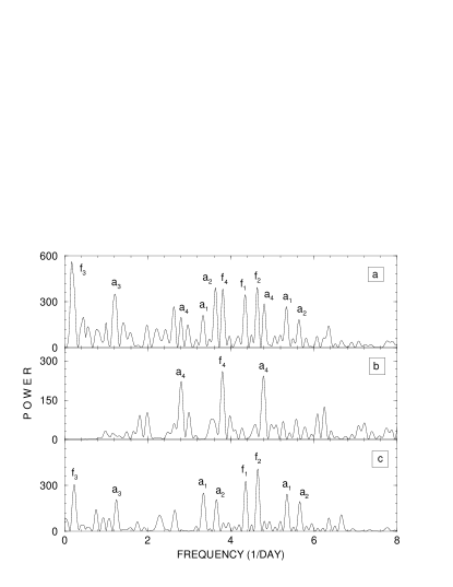
Figure 3: Power spectra of Set 10. (a) Raw data; In addition to the three previously known periods – the orbital period (marked as f₁), the negative superhump (f₂) and the beat between the two (f₃), there is a fourth structure of peaks centered around 6.3 h (f₄); ‘a_i’ ($i=1-4$) represent 1 d^-1 aliases of ‘f_i’ correspondingly; (b) After fitting and subtracting f₁, f₂, f₃ and the nightly trends, the period is still present, and becomes the strongest peak in the graph. (c) A synthetic light curve, consisting of sinusoids of the three previously known optical periods (5.2 h, 5.5 h, 4 d) (plus noise) sampled as the data thus illustrating the window function. This test shows that aliases of the three known periods cannot explain the f₄ peak.

In Fig. 4 we show the data of Set 10 folded on the 6.3-h period after the three previously known periods (5.2 h, 5.5 h and 4-d) were removed. The peak-to-peak amplitude of the sinusoidal fit to the light curve is $0.08\pm 0.01$ mag.

Figure 4: The 2001 January data (after the outburst) folded on the 6.3-h period and binned into 20 bins. Two cycles are shown for clarity. The bars represent 1-$\sigma$ errors in each bin.

3.3 Other subsets

Figure 5 presents power spectra of the five best sets among all ten. Sets 1, 2, 3, 5 and 8 were rejected because either outbursts occurred during the observations (Sets 3 and 8), and the data between outbursts were too scarce; the mean night length was too short (Sets 1, 2 and 8) or there were long gaps during the runs (Sets 1, 3 and 5). The three previously known periods (5.2 h, 5.5 h, 4 d) have been removed, as have the nightly trends. In the residual power spectra of Sets 4, 6 and 7, the highest peak (or a 1 d^-1 alias) is compatible with the peak from Set 10. It is absent from Set 9, which is one of the best data sets, but only gives an upper limit of 0.02 mag on the peak-to-peak amplitude of the 6.3-h period in these data. We return to this issue below.

Figure 5: Power spectra of the best five subsets after the removal of the three previously known periods (5.2 h, 5.5 h, 4 d) and a linear fit from each night. In Sets 4, 6 and 7 the strongest peak (or a 1 d^-1 alias) is consistent with the location of the peak found in Set 10 (which is identical with Fig. 3b). Its 1 d^-1 aliases (a₄) are also marked. Set 9 do not show this pattern despite presumably being one of the best sets. This issue is further discussed below. The vertical dotted line shows the mean of the period found from the four other data sets.

In Sets 4, 6, 7 and 10 the f₄-peak lies in the range 3.74–3.84 d^-1 ($0.2639\pm 0.0035$ d). The large interval originates from many observations covering less than a full cycle of the period (thus being affected by the detrending method used), but might also reflect true long-term changes in the periodicity. Note that superhumps in other systems have shown large changes (e.g., up to more than one per cent in V603 Aql – Patterson et al. 1997).

3.4 Tests

To reject the possibility that individual nights may be responsible for the appearance of the period, we calculated power spectra for the data from Sets 6 and 10 while rejecting one night at a time. The suspected period survived this test and was one of the four highest peaks, together with the 5.2-h, 5.5-h and 4-d periods (besides 1 d^-1 aliases). In addition, when the data in Set 10 were divided into two independent sets consisting the even nights and odd nights, the 6.3-h period appeared in both sets.

We investigated other possible spurious sources of the candidate period, in a series of tests detailed below. We first assessed whether the period could be an artefact of the window function in combination with the known periods. We then tested whether noise, either uncorrelated or correlated, could be the source of the periodicity. We then considered the possibility that extinction may be responsible for the appearance of the period. Finally, we comment on the fact that the superhump periodicity in TV Col was discovered in published observations and subsequently confirmed by the new data.

3.4.1 The window function

Could the new peak in the power spectrum be an artefact of the window function? To check this we created a noiseless simulation of two of the best sets (6 and 10). A synthetic light curve was built using three sinusoids at the orbital period, the negative superhump period and at the beat period between the two. These sinusoids were given the same amplitudes they have in the data, and sampled according to the window function. There was no evidence for significant power at the proposed period.

3.4.2 Uncorrelated noise

To check whether uncorrelated noise could be responsible for the presence of the candidate period, we added noise to the model light curves of Sets 6 and 10 (previous section). The noise in the original data was defined as the root mean square of the data minus the three periods modelled. We then searched for the highest peak in a small interval (3.72–4.00 d^-1) around the candidate period. In 1000 simulations, no peak reached the height of the candidate periodicity. An individual example of a simulation for Set 10 is shown in Fig. 3c. In a further test we mimicked the technique shown in Fig. 3b, by subtracting the previously known periods (5.2 h, 5.5 h, 4 d) from our model light curves, after imposing an error of 0.005 d^-1 in the periods. We then checked the height of the highest peak in the resulting power spectrum. In 1000 simulations, no peak reached the level of the candidate periodicity.

3.4.3 Correlated noise

We also tried to assess the probability that correlated noise could be responsible for the candidate periodicity. In the absence of a model for the correlated noise, the best test is to use the repeatability between different data sets. Given that we found a period in Set 10, and assuming that the nearby peak in Set 4 represents the same period, we can ask how likely it is that the strongest period in the other data sets (after the previously known periods had been subtracted) would be consistent with it. The probability of the highest peak in another data set being, by chance, compatible with the candidate period in Set 10 is 0.1. This was calculated from (i) the frequency range for the candidate period on the assumption that the peaks in Set 4 and Set 10 set this range, which implies that the peaks are compatible if they are within 0.1 d^-1, and (ii) the range over which it could occur taken as the spacing of the 1 d^-1 aliases (1 d^-1 is the maximum range over which periods are truly independent). The period discovered in Set 10 was seen in two of the remaining three data sets (besides Set 4). We thus used the binomial distribution to find that the probability of this occurring by chance was only about 2.8 per cent.

3.4.4 Extinction effects

The observations were made in white light, and the differential photometry was performed relative to three comparison stars that are almost certainly redder than TV Col. Since there are very few blue stars available in a typical CV field, this is a standard procedure in CCD photometry of CVs. The colour difference may result in extinction variations with airmass on the data. For a single observing site this could introduce apparent periodicities in the data which should approximately be equal to a fraction of a day, i.e. a period of 12 h, 8 h, 6 h, etc. This might explain the detection of a 6.3 h, although the typical length of the observing runs would more favour a period of 8 or 12 h. However, it is very unlikely that two different data sets would be affected by extinction variations such that the same period is found in both. Furthermore, the observations in data set 10 were in fact obtained at different observing sites, where the source will cross the meridian at very different times, which are far from being equal an integral number of the new period we found.

It is important to realise that variations in the data due to extinction are not intrinsic to the source, i.e. this will distort the light curve and will actually affect the detection of any period that is present in the source. In fact, we do detect the previously known 5.2 and 5.5-h periods at the correct positions in the power spectra, so this effect cannot be strong. As shown in Fig. 3, we detect the 5.2, 5.5 and 6.3-h periods at very similar strengths in data set 10, and it is unclear how one could reject the detection of the 6.3-h period without having to discard the 5.2 and 5.5-h periods as well. Nevertheless, as a final test we fitted and subtracted a sinusoid corresponding to the sidereal day ($23^{h}56^{m}4^{s}$) from the SA data and checked the resulting power spectrum. The candidate period survived this test, which confirmed that extinction effects are not responsible for the presence of the 6.3-h period.

3.4.5 Confirmation from new observations

Finally, we note that we have previously argued for a 6.3-h periodicity when we had only the data sets 1–8 (Retter & Hellier 2000; Retter et al. 2001). Its presence has now been confirmed by the new data. Table 3 summarizes all periods detected in the light curve of TV Col.

Table 3: The periods of TV Col

Number	Period [d]	Nature	Reference
1	0.022112(58)	spin	Schrijver et al. (1985; 1987)
2	0.21627(7)	negative	Motch (1981)
	0.21631(1)	superhump	Hutchings et al. (1981)
	0.216325(1)		Barrett et al. (1988)
	0.2162774(14)		Hellier et al. (1991)
	0.2162783(12)		Hellier (1993)
	0.216036(93)		Augusteijn et al. (1994)
3	0.228600(5)	orbital	Hutchings et al. (1981)
	0.228685(3)		Barrett et al. (1988)
	0.2285529(2)		Hellier et al. (1991)
	0.2286034(16)		Hellier (1993)
	0.22859884(77)		Augusteijn et al. (1994)
4	0.2639(35)	positive	This work
		superhump
5	3.90(15)	nodal	Motch (1981)
	4.024(4)	precession	Hutchings et al. (1981)
	4.02603(3)		Barrett et al. (1988)
	4.0283(5)		Hellier et al. (1991)
	3.934(70)		Augusteijn et al. (1994)

4 Discussion

4.1 The new period

The photometric data show a periodicity of 0.2639 d, in addition to the previously known periods. The repeatability of the peak in several independent data sets makes it highly significant, and it is also comforting to note that the new period is generally seen best in the best data sets.

The 6.3-h period has almost exactly the value predicted from the relation of Stolz & Schoembs (1984; updated by Patterson 1999), which is shown in Fig. 6. TV Col has already been classified as a permanent superhump system because its 5.2-h period was interpreted as a negative superhump (Section 1.2). Moreover, the new period and the negative superhump obey the relation between the two types of superhumps mentioned in Section 1.3. Further support for this idea (although not completely independently) comes from the fact that TV Col obeys a recently-proposed relation between the orbital period and the ratio between the positive superhump excess over the negative superhump deficit (Retter et al. 2002). Therefore, the new period is naturally interpreted as a positive superhump.

Figure 6: The relation between superhump period excess (over the orbital period) and orbital period in superhump systems. Empty circles correspond to periods in the SU UMa systems. Filled circles represent the values in permanent superhumpers. The data were taken from Patterson (1998; 1999). The solid line represents the linear fit to the data. The two tilted dashed lines show the 1-$\sigma$ error. There are a few permanent superhump systems with periods above the upper edge of the period gap (as defined by Diaz & Bruch 1997), marked by the vertical long-dashed line. The new period detected in TV Col obeys the relation and significantly extends the range of superhump periods in CVs.

Our result supports the observational connection between positive and negative superhumps. Since almost every permanent superhump system that has been well studied over a few years shows both types of superhumps, we may speculate that this is the general behaviour among permanent superhump systems. The idea that the two types of superhumps have a similar physical origin, namely a precessing accretion disc, is also supported.

4.2 Changes through the outburst

TV Col had a mini-outburst on 2001, January 7 (Section 2.2; Fig. 1). Such outbursts are very common in the light curve of TV Col, but their nature is still unclear (Szkody & Mateo 1984; Schwartz et al. 1988; Angelini & Verbunt 1989; Hellier & Buckley 1993; Augusteijn et al. 1994; Kato 2001a; 2001b).

Examination of the data presented above shows that the 6.3-h period appeared only in the data taken after the 2001 outburst (Set 10). Before the outburst (Set 9) an upper limit of 0.02 mag is found for the peak-to-peak amplitude of this periodicity. It is thus possible that the amplitude was increased by the outburst by at least a factor of four. Alternatively, the outburst triggered the appearance of the positive superhump period. We note that amplitudes of permanent superhumps can significantly vary in a single source and sometimes the superhumps are even not detected (e.g. Patterson et al. 1997). The amplitude of the negative superhump, on the other hand, was slightly lower after the outburst. Table 4 presents the development of the amplitudes of the four periods through the outburst. The data are consistent with there being no change in the amplitudes of the 5.5-h and 4-d periods.

Table 4: Changes in the amplitudes of the periods by the outburst

Period	Peak-to-peak amplitude	Peak-to-peak amplitude
	before outburst (Set 9)	after outburst (Set 10)
5.2 h	0.09(1)	0.06(1)
5.5 h	0.10(2)	0.10(2)
6.3 h	$<$0.02	0.08(1)
4 d	0.22(6)	0.21(4)

Previous studies around an outburst in 1991 December showed that the phase of the 5.2-h period (the negative superhump) was changed by about 0.4 (Hellier & Buckley 1993). Our 2001 data were similarly checked. First, the ephemeris fitted to the two parts of the data (before and after outburst) suggested a shift of $\sim$1.4 h (0.27 cycles). To confirm this result, minima of the negative superhump were calculated from the data after the subtraction of the other periods (4 d and 5.5 h from both sets, and 6.3 h only from the latter data). The O$-$C diagram (Fig. 7) clearly shows a shift of $\sim$1.2 h or 0.24 cycles. The data are consistent with no shift in the phase of the orbital and beat periods. Note that the errors on the 4-d period and its phase are large as less than two cycles of this frequency were observed in each set.

Figure 7: O$-$C diagram of the minima of the negative superhump period. The other periods were first subtracted from the data. A parabola was fitted to the light curve near the minima to find the points of extrema. The dashed vertical line presents the time of the outburst. The two horizontal lines show the mean of the points before and after the outburst. The phase of the negative superhump was shifted by $\sim$0.25 by the outburst.

4.3 The mass ratio problem

According to theory, superhumps can only appear in binaries with tidally unstable accretion discs. Simulations show that the tidal instability can only occur if the disc radius exceeds a certain value, the 3:1 resonance radius. This implies that eccentric discs (which generate the superhumps) can be present only in CVs with small mass ratios – $q$=$M_{donor}/M_{compact}$$\la$0.33 (Whitehurst 1988; Whitehurst & King 1991; Murray 2000). Hellier (1993) concluded, however, that the mass ratio in TV Col is $q$=0.62-0.93 from a spectroscopic analysis of the system, but this depended on an interpretation of the radial velocity variation of the emission lines that may not be correct.

We can estimate the mass ratio in TV Col by a different method. The relation between the orbital period and the superhump period excess (Fig. 6) suggests that there is a connection between the latter and some physical quantity. Indeed, this relation was initially explained by Osaki (1985), who investigated the motion of free particles in the binary potential. He considered the axisymmetric part of the tidal perturbation potential of the secondary star and derived an expression for the precession rate of the eccentric disc based on a nonresonant free particle orbit at the disc edge in the first order. His formula has been commonly used to obtain the binary mass ratio from the superhump period excess (e.g. Retter, Leibowitz & Ofek 1997; Patterson 1998). The superhump period in TV Col is $15.4\pm 1.5$ per cent larger than the orbital period. Using equation (15) of Osaki (1996), we find: $q=0.92\pm 0.12$ – well above the 0.33 limit suggested by the hydrodynamic simulations, and consistent with the values estimated by Hellier (1993) presented above.

The mass ratio in TV Col might thus be inconsistent with the models. In the following, we discuss a few possible solutions for this dilemma and suggest how the observations of TV Col can be reconciled with the theory.

4.3.1 TV Col may be an extreme system

TV Col has a binary period of 5.5 h. According to the relation between the orbital period and the secondary mass in CVs (Smith & Dhillon 1998), the companion mass is $M_{2}=0.57\pm 0.11M_{\odot}$. If the mass of the primary white dwarf in TV Col is $M_{1}\approx 1M_{\odot}$ (Ramsay 2000), the mass ratio is around 0.6 – still above the theoretical limit. TV Col can have a mass ratio below the critical value only for the secondary mass at the bottom of the above range and for a very massive white dwarf near the Chandrasekhar mass (1.44$M_{\odot}$). The mass ratio is then 0.32. However, for a CV with the limiting theoretical mass ratio of 0.33, a superhump period excess of only about 7 per cent is expected according to Osaki’s equation discussed in the previous section and this is inconsistent with the observational value of TV Col. This fact might indicate that Osaki’s formula cannot be applied to TV Col.

The equation developed by Osaki is based on a dynamical calculation of non-resonant particles. Furthermore, it does not assume that the disc radius exceeds the 3:1 resonance radius. More sophisticated models have been introduced since. Murray (2000) compared the mass ratios reliably measured for three eclipsing SU UMa systems with estimates using the superhump excess in Osaki’s equation and found some inconsistency. He argued that the use of a gaseous disc (rather than isolated test particles) modifies the equations. The eccentricity is excited at the 3:1 resonance and then propagates inwards through the disc. According to his ideas, pressure forces are an important factor in the calculations, yielding mass ratios lower than the previous estimates. Murray also argued that, for systems with mass ratios exceeding 0.25, the dynamical equations cannot be applied. From his simulations (see his fig. 2), and using the observed superhump period excess of TV Col, a mass ratio of about 0.3 can be deduced. For a white dwarf of $M_{1}=1M_{\odot}$, this implies an undermassive secondary with $M_{2}=0.3M_{\odot}$, which would indicate an evolved star close or near the end of hydrogen burning (see discussions in Augusteijn et al. 1996; Beuermann et al. 1998).

Montgomery (2001) and Montgomery et al. (in preparation) developed analytic expressions for both types of superhumps. Montgomery et al. argued that in binaries having superhumps, the ratio between the negative superhump deficit and the positive superhump excess ($\phi=\epsilon_{-}/\epsilon_{+}$) should be used to estimate the mass ratio, rather than just one of these parameters. Using their equation 9 and the observed $\phi$ parameter in TV Col ($-0.357\pm 0.055$), we can estimate a mass ratio within the range 0.31-0.56. The lower value is consistent with Murray’s simulations.

The mass ratio in TV Col may thus be about the critical limit of 0.33. A criticism of this solution is that it suggests that it is only a coincidence that TV Col obeys the apparent relation between the superhump period excess and the orbital period (Fig. 6).

4.3.2 Invoking the magnetic field of the white dwarf

Another solution to the problem might come from the suggestion that the strong magnetic field of the white dwarf pushes the particles in the outer accretion disc to larger orbits, allowing a disc size bigger than the normal tidal radius in a non-magnetic system (this was confirmed by Murray, personal communication). In this way tidally unstable discs in systems with mass ratios larger than 0.33 can be obtained. We are, however, not familiar with any model calculations that have been made for this case.

5 Summary and conclusions

1. We have found a 6.3-h period in the optical light curve of TV Col in the multi-longitude photometric campaign held in 2001 January. This detection confirms our findings from re-analysis of previously published photometric data. The periodicity is most naturally explained as a positive superhump.

2. In the middle of the 2001 January run a short-lived minor outburst occurred. The new period is seen only in the data following outburst. The outburst also changed the phase of the negative superhump by about a quarter of a cycle, while its amplitude was slightly decreased.

3. Our findings support the classification of TV Col as a permanent superhump system. Its superhump period is the longest known among CVs. TV Col thus offers a unique opportunity to test and reject some of the models, as it extends the superhump regime to periods far beyond the predicted values into a regime where the differences between models become significant. The mass ratio of TV Col might exceed the limit for superhump systems allowed by hydrodynamic simulations.

4. The observational and physical link between positive and negative superhumps is thus strengthened by our result. We might speculate that all permanent superhump systems may have both types of superhumps.

5. Our finding significantly extends the upper limit of orbital periods in positive superhump systems (from 3.7 h to 5.5 h). This range of periods is populated with dwarf novae and nova-like systems. Therefore, we strongly urge observers to search for superhumps in nova-likes and dwarf novae with orbital periods above the period gap and up to at least 5.5 h, to check whether TV Col is unique. If TV Col has certain properties that can explain its extraordinarily long superhump period (e.g. classification as an intermediate polar), then other long-period superhump systems should possess similar features.

6 Acknowledgments

This paper uses observations made at the South African Astronomical Observatory (SAAO). We thank P. Woudt for his kind assistance as the support astronomer, J. Patterson for utilizing the CBA net and Michele Montgomery for sending us an early version of her paper prior to publication. Two anonymous referees are acknowledged for valuable comments. We also thank D. O’Donoghue for sending some of the data to CH and for using his reduction software. TN was a PPARC advanced fellow when the majority of this work was carried out. AR was supported by PPARC and is currently supported by the Australian Research Council.

References

- [1] Angelini L., Verbunt F., 1989, MNRAS, 238, 697
- [2] Arenas J., Catalan M.S., Augusteijn T., Retter A., 2000, MNRAS, 311, 135
- [3] Augusteijn T., Heemskerk M.H.M., Zwarthoed G.A.A., van Paradijs J., 1994, A&A Suppl., 107, 219
- [4] Augusteijn T., van der Hooft F., de Jong J.A., van Paradijs J., 1996, A&A, 311, 889
- [5] Baba et al., 2002, PASJ, 54, L7
- [6] Barrett P., O’Donoghue D., Warner B., 1988, MNRAS, 233, 759
- [7] Beuermann K., Baraffe I., Kolb U., Weichhold M., 1998, A&A, 339, 518
- [8] Bonnet-Bidaud J.M., Motch C., Mouchet M., 1985, A&A, 143, 313
- [9] Diaz M.P., Bruch A., 1997, A&A, 322, 807
- [10] Hellier C., 1993, MNRAS, 264, 132
- [11] Hellier C., 1996, in Evans A., Wood J.H., eds., Proc. IAU Colloq. 158, Cataclysmic variables and related objects, Kluwer, Dordrecht, 143
- [12] Hellier C., Buckley D.A.H., 1993, MNRAS, 265, 766
- [13] Hellier C., Mason K.O., Mittaz J.P.D., 1991, MNRAS, 248, 5
- [14] Hutchings J.B., Crampton D., Cowley A.P., Thorstensen J.R., Charles P.A., 1981, ApJ, 249, 680
- [15] Kato T., 2001a, vsnet-alert, 5532, http://www.kusastro.kyoto-u.ac.jp/vsnet/Mail/vsnet-alert/msg05532.html
- [16] Kato T., 2001b, vsnet-alert, 5589, http://www.kusastro.kyoto-u.ac.jp/vsnet/Mail/vsnet-alert/msg05589.html
- [17] McArthur B.E. et al., 2001, ApJ, 560, 907
- [18] Montgomery M.M., 2001, MNRAS, 325, 761
- [19] Motch C., 1981, A&A, 100, 277.
- [20] Murray J.R., 2000, MNRAS, 314, L1
- [21] Murray J.R., Armitage P.J., 1998, MNRAS, 300, 561
- [22] Murray J.R., Chakrabarty D., Wynn G.A., Kramer L., 2002, MNRAS, 335, 247
- [23] Osaki Y., 1985, A&A, 144, 369
- [24] Osaki Y., 1996, PASP, 108, 39
- [25] Patterson J., 1994, PASP, 106, 209
- [26] Patterson J., 1998, PASP, 110, 1132
- [27] Patterson J., 1999, in Mineshige S., Wheeler C., eds, Disk Instabilities in Close Binary Systems, Universal Academy Press, Tokyo, Japan, p. 61
- [28] Patterson J., Richman H., 1991, PASP, 103, 735
- [29] Patterson J., Thomas G.R., Skillman D., Diaz M., Suleimanov V.F., 1993, ApJ Suppl., 86, 235
- [30] Patterson J., Kemp J., Saad J., Skillman D., Harvey D., Fried R., Thorstensen J.R., Ashley R., 1997, PASP, 109, 468.
- [31] Ramsay G., 2000, MNRAS, 314, 403
- [32] Retter A., Hellier C., 2000, in Charles P., King A., O’Donoghue D., eds, Proc. of Cataclysmic Variables: a 60th Birthday Symposium in Honour of Brian Warner, special edition, p35
- [33] Retter A., Naylor T., 2000, MNRAS, 319, 510
- [34] Retter A., Leibowitz E.M., Naylor T., 1999, MNRAS, 308, 140
- [35] Retter A., Leibowitz E.M., Ofek E.O., 1997, MNRAS, 286, 745
- [36] Retter A., Hellier C., Augusteijn T., Naylor T., 2001, ASP Conf. Ser., Vol 229, ”Evolution of Binary and Multiple Star Systems: a Meeting in Celebration of Peter Eggleton’s 60th Birthday”, eds. Ph. Podsiadlowski, S. Rappaport, A. R. King, F. D’Antona, L. Burderi (San Francisco: ASP), p. 391.
- [37] Retter A., Chou Y., Bedding T., Naylor T., 2002, MNRAS, 330, L37
- [38] Scargle J.D., 1982, ApJ, 263, 835
- [39] Schrijver J., Brinkman A.C., van der Woerd H., Watson M.G., King A.R., van Paradijs J., van der Klis M., 1985, SSRv, 40, 121
- [40] Schrijver J., Brinkman A.C., van der Woerd H., 1987, ApSS, 130, 261
- [41] Schwarz H.E., van Amerongen S., Heemskerk M.H.M., van Paradijs J., 1988, A&A, 202, L16
- [42] Smith D.A., Dhillon V.S., 1998, MNRAS, 301, 767
- [43] Steeghs D., Harlaftis E.T., Horne K., 1997, MNRAS, 290, L28
- [44] Stolz B., Schoembs R., 1984, A&A, 132, 187
- [45] Szkody P., Mateo M., 1984, ApJ, 280, 729
- [46] Warner B., 1995, Cataclysmic Variable Stars, Cambridge University Press, Cambridge
- [47] Warner B., 1996, Ap&SS, 241, 263
- [48] Whitehurst R., 1988, MNRAS, 232, 35
- [49] Whitehurst R., King A., 1991, MNRAS, 249, 25
- [50] Wood M.A., Montgomery M.M., Simpson J.C., 2000, ApJ, 535, L39