Abstract

We present an overview of all the cosmic shear results obtained so far. We focus on the 2-point statistics only. Evidences supporting the cosmological origin of the measured signal are reviewed, and issues related to various systematics are discussed.

Cosmic shear review

¹Institut d’Astrophysique de Paris, CNRS, 98bis Boulevard Arago, F–75014 Paris.
²University of Lisboa, Dept. of Physics, 1749-016, Lisboa.
³Obs. de Paris/LERMA, 77 Av. Denfert-Rochereau, F–75014 Paris.
⁴Service de Physique Théorique de Saclay, F–91191 Gif sur Yvette Cedex.

1 Introduction

The cosmic shear is a gravitational lensing effect caused by the large scale structures in the universe on the distant galaxies. Its net effect is to distort coherently the galaxy images over large angular scales and to change the focusing properties of the light beam (galaxies appear larger or smaller depending on the intervening mass density). Only the former effect is ’easily’ measurable, and is the one we will discuss here. The latter, which has been measured in some cluster lensing cases, is much more challenging for cosmic shear purposes.

The measurement of the amplitude of the cosmic shear as a function of scale is a direct indicator of the projected mass power spectrum, convolved with a selection function which only depends on the cosmological parameters and the redshift distribution of the sources. It is therefore a tool for evaluating the mass distribution in the universe, as well as for measuring the cosmological parameters. In the following, we first outline the theory of cosmic shear, and its link to measurable quantities in Section2. We discuss the measurements and the systematics in Section 3. Section 4 is a discussion of the cosmological parameters measurements and the still open problems associated with it.

2 Theory

In the presence of mass inhomogeneities, a light ray is deflected, and it is observed at an angular position $\beta$ on the sky instead of at its intrinsic location $\theta$. The mapping between the two position angles defines the amplification matrix $\cal A$

$${\cal A}={\partial\beta_{i}\over\partial\theta_{j}}=\left(\matrix{1-\kappa-\gamma_{1}\ \ \ \ \ \ \ \gamma_{2}\cr\gamma_{2}\ \ \ \ \ \ \ 1-\kappa+\gamma_{1}}\right),$$ (1)

where the convergence $\kappa$ and the shear ${{\mbox{\boldmath$\gamma$}}}=(\gamma_{1},\gamma_{2})$ are given by the second derivatives of the projected gravitational potential $\varphi$:

$$\kappa={1\over 2}\left(\varphi_{,11}+\varphi_{,22}\right)\ ;\ \ \gamma_{1}={1\over 2}\left(\varphi_{,11}-\varphi_{,22}\right)\ ;\ \ \gamma_{2}=\varphi_{,12}.$$ (2)

Figure 1: The left panel is a 3-dimensional mass power spectrum for the linear (dashed) and non-linear (solid) regimes when baryons are included. A value of $\Omega_{b}=0.05$ was used. The right panel shows the induced convergence power spectrum (Eq.3) for the two dynamical regimes. Other parameters are $\Omega_{\rm cdm}=0.25,\Omega_{\Lambda}=0.7,\sigma_{8}=0.9,h=0.7,z_{\rm source}=0.8$.

The central quantity in cosmic shear analysis is the convergence power spectrum $P_{\kappa}(k)$, which relates any cosmic shear two point statistics to the cosmological parameters and the 3-dimensional mass power spectrum $P_{3D}(k)$:

$$P_{\kappa}(k)={9\over 4}\Omega_{0}^{2}\int_{0}^{w_{H}}{{\rm d}w\over a^{2}(w)}P_{3D}\left({k\over f_{K}(w)};w\right)\left[\int_{w}^{w_{H}}{\rm d}w^{\prime}n(w^{\prime}){f_{K}(w^{\prime}-w)\over f_{K}(w^{\prime})}\right]^{2},$$ (3)

where $f_{K}(w)$ is the comoving angular diameter distance out to a distance $w$ ($w_{H}$ is the horizon distance), and $n(w(z))$ is the redshift distribution of the sources. The mass power spectrum $P_{3D}(k)$ is evaluated in the non-linear regime [24], and $k$ is the 2-dimensional wave vector perpendicular to the line-of-sight. Figure 1 is an example of 3-dimensional and convergence power spectra for comparison. A fair amount of baryons was included (using CAMB [17]), in order to show that the baryon oscillations, which are clearly visible on the 3D spectrum, are severely diluted in the projected spectrum.

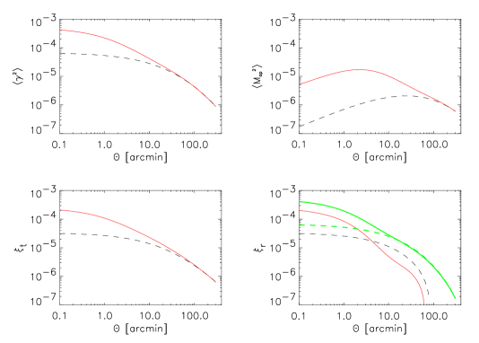
Figure 2: Lensing statistics predictions for the cosmological model used in Figure 1. Both linear (dashed) and non-linear (solid lines) regimes are represented. On the bottom-right plot, the thick dashed and solid lines are the full shear correlation function.

The cosmic shear effect is measured from the ellipticity $e$ of the galaxies, which is assumed to be fully described by their second order moments ${\cal M}$ of the surface brightness $I({{\mbox{\boldmath$\theta$}}})$:

$${\cal M}_{ij}=\int I\left({{\mbox{\boldmath$\theta$}}}\right)\theta_{i}\ \theta_{j}\ {\rm d}^{2}\theta\ ;\ \ \ {{\mbox{\boldmath$e$}}}=\left({{\cal M}_{11}-{\cal M}_{22}\over{\rm Tr}({\cal M})},\ \ {2{\cal M}_{12}\over{\rm Tr}({\cal M})}\right).$$ (4)

To first order in the lensing amplitude, $e$ is an unbiased estimate of the shear $\gamma$. The three most commonly measured 2-point statistics are respectively the shear top-hat variance [19, 1, 13], the aperture mass variance [14, 23] and the shear correlation function [19, 1, 13]. They are all different measurements of the same quantity, the convergence power spectrum $P_{\kappa}(k)$:

$$\langle\gamma^{2}\rangle={2\over\pi\theta_{c}^{2}}\int_{0}^{\infty}~{}{{\rm d}k\over k}P_{\kappa}(k)[J_{1}(k\theta_{c})]^{2}\ ;\ \ \langle M_{\rm ap}^{2}\rangle={288\over\pi\theta_{c}^{4}}\int_{0}^{\infty}~{}{{\rm d}k\over k^{3}}P_{\kappa}(k)[J_{4}(k\theta_{c})]^{2},$$

$$\xi(\theta_{c}) = \langle{{\mbox{\boldmath$\gamma$}}}(r)\cdot{{\mbox{\boldmath$\gamma$}}}(r+\theta_{c})\rangle_{r}={1\over 2\pi}\int_{0}^{\infty}~{}{\rm d}k~{}kP_{\kappa}(k)J_{0}(k\theta_{c})$$ (5)

$$\left(\matrix{\xi_{t}(\theta_{c})\cr\xi_{r}(\theta_{c})}\right) = {1\over 4\pi}\int_{0}^{\infty}~{}{\rm d}k~{}kP_{\kappa}(k)\left[J_{0}(k\theta_{c})\pm J_{4}(k\theta_{c})\right]$$ (6)

where $J_{n}$ is the Bessel function of the first kind, and $\theta_{c}$ is the smoothing radius (or the pair separation for the shear correlation functions).

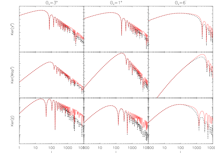
Figure 3: Integrants of the different lensing statistics (Eqs.(2,6)) for the linear (dotted line) and non-linear (solid line) regimes. From top to bottom: top-hat variance, aperture mass and total correlation function. The vertical axis is arbitrary, and the three columns correspond to $\theta_{c}=3{\rm deg}$, $1{\rm deg}$ and $6^{\prime}$ respectively.

Figure 2 is an example of lensing quantities predictions for the same cosmology as in Figure 1. It shows the importance of the non-linear corrections for scales below $30^{\prime}$ to $1$ degree. An illustration of the difference between the linear and non-linear regimes is done by plotting the integrants of Eqs.(2, 6) as in Figure 3. Figures 2 and 3 make it clear that the lensing signal is dominated by the first few peaks in the smoothing kernel, with a transition linear/non-linear around a smoothing scale of $1$ degree, depending slightly on the statistic under interest.

3 Observations

3.1 Two-point statistics

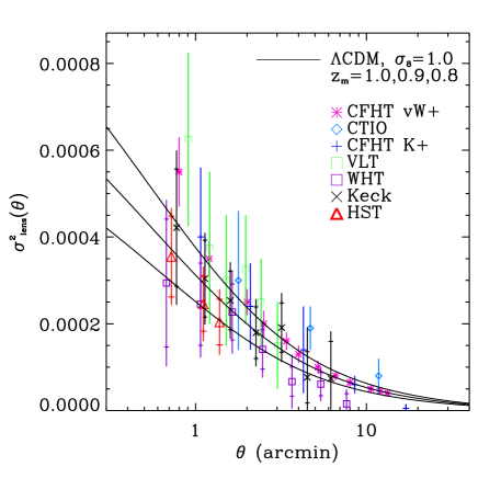
Figure 4: Compilation of recent results of top-hat shear variance measurements from several groups [21].

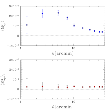
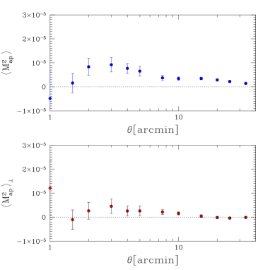
Figure 5: Left: $E$ (top) and $B$ (bottom) modes measured in the VIRMOS survey. Right: $E$ (top) and $B$ (bottom) modes measured in the RCS survey. The $B$ mode is low and the $E$ mode compatible with the predictions for the aperture mass statistics.

There are now several evidences of the cosmological origin of the measured signal:

(a) The consistency of the shear excess variance measured from different telescopes, at different depths and with different filters. This is summarized on Figure 4.

(b) On a single survey, the self consistency of the different types of lensing statistics as given in Eqs.(2,6) [27].

(c) The $E$, $B$ modes decomposition separates the lensing signal into curl and curl-free modes [5]. It is expected, and it can also be quantified on the star field [28], that residual systematics equally contribute to $E$ and $B$, while the lensing signal should be present ONLY in the $E$ mode. This is a consequence that gravity derives from a true scalar field [25]. The $E$ mode is identical to the aperture mass statistic Eq.(2) [14, 23], while the $B$ mode can be computed in the same way by rotating each galaxy by $45$ degrees. The $E$ and $B$ modes have been measured in several surveys [27, 28, 20, 9, 4], and support the cosmological origin of the signal, showing also the already small amount of residual systematics achieved with today’s technology. Figure 5 shows such measurements for the VIRMOS–DESCART and RCS surveys.

(d) The lensing signal is expected to decrease for low redshift sources, as consequence of the lower efficiency of the the gravitational distortion. This decrease of the signal has been observed recently for the first time, when comparing the VIRMOS survey aperture mass [28] which has a source mean redshift around $0.9$ to the RCS which has a source mean redshift around $0.6$. The expected decrease in signal amplitude is about $2$, which is what is observed (see Figure 5).

(e) Space images provide in principle a systematics-free environment, and even if the observed areas are still smaller than ground based observations, space data provide ideal calibrations of the cosmic shear signal [22, 7, 21], which are in excellent agreement with ground based measurements.

3.2 Systematics

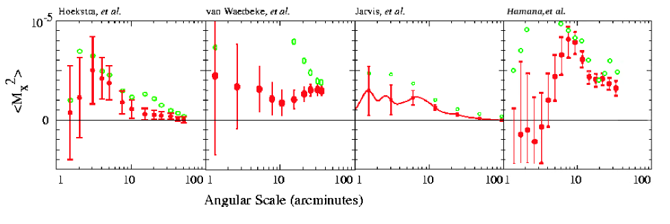
Figure 6: Plot showing the relative amplitude of the $E$ and $B$ modes (points without and with error bars respectively) for the surveys where the aperture mass has been measured [9, 28, 12, 6] (picture taken from [12], and extended) The result of [9] is for the full magnitude range, while in Figure 5, right panel, it is for the galaxies used for the cosmic shear analysis.

As we said, any 2-points statistic can be decomposed into the so-called $E$ and $B$ modes channels, which separate the cosmological signal from the systematics [5, 20]. Figure 6 shows the $E$ and $B$ modes that have been measured so far, using the aperture mass only (this is the statistic which provides an unambiguous $E$ and $B$ separation [20]). The two deepest surveys have large scale $B$ mode contamination [28, 6], and the two shallow surveys have small scale contamination [9, 12].

The source of systematics is still unclear. It could come in part from an imperfect Point Spread Function correction, but also from intrinsic alignment of galaxies. The later effect has been observed for dark matter halos in simulations, but it is still difficult to have a reliable prediction of its amplitude. Nevertheless, it is not believed to be higher than a $10\%$ contribution for a lensing survey with a mean source redshift at $z_{s}=1$. In any case, intrinsic alignment contamination can be removed completely by measuring the signal correlation between distant redshift bins, instead of measuring the full projected signal [16].

4 Cosmological Parameters Constraints and Conclusion

As quoted earlier [11], the cosmic shear signal depends primarily on four parameters: the cosmological mean density $\Omega_{m}$, the mass power spectrum normalization $\sigma_{8}$, the shape of the power spectrum $\Gamma$, and the redshift of the sources $z_{s}$. Therefore, any measurement of the statistics shown in Section 2 provide constraints on these parameters. A big enough lensing survey [10] will also provide constraints on many other parameters, but we do not discuss this issue here.

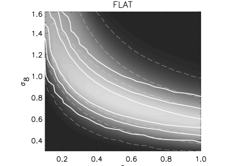
Figure 7: The solid lines on each plot show the 1, 2 and 3$\sigma$ contours of the VIRMOS and RCS survey, from the measurements shown in Figure 5. The contours have been marginalised over the source redshift and the slope of the matter power spectrum as described elsewhere [27, 9].

Figure 7 shows the joint $\Omega_{m}$, $\sigma_{8}$ constraints obtained from the measurements of Figure 5. They are obtained only when comparing the measured lensing signal to the non-linear predictions. Indeed, the actual surveys are not yet big enough to probe the linear scales accurately. The non-linear power can be computed numerically [24], but its precision is still uncertain. Recent investigations show that a $10\%$ r.m.s. uncertainty is expected, which means that the cosmological parameters cannot be known with better precision for the moment. According to the Figures 2, 3, the transition scale between the linear and non-linear regimes is around 1 degree. The consequence is that the quoted mass normalization $\sigma_{8}$ is sensitive to the validity of the non-linear mapping at small scale. In this respect, [12] are less contaminated by this problem because they used the lensing signal from $30^{\prime}$ to $100^{\prime}$ to constrain the mass normalization.

Table 1 summarizes the $\sigma_{8}$ measurements for all the lensing surveys published so far. For simplicity it is given for $\Omega_{m}=0.3$. Despite the differences among the surveys, it is worth to note that the results are all consistent within $2.5\sigma$ between the most extreme cases, when poorly known parameters are marginalised.

The residual $B$ mode has been included in the analysis of the most recent cosmic shear surveys [28, 9, 6, 12], but we do not know yet how to deal with it properly: some groups [28, 9, 6] added the $B$ mode in quadrature to the $E$ errors, taking into account the correlation between various scales. The $B$ mode has been substracted first from the $E$ mode in [9], and not in [28]. This might probably result in a slight bias for high $\sigma_{8}$ values in [28]. Unfortunately we have no garantee that the $B$ substraction is the right correction method. Recently [12] marginalised the probabilities over $E-B$ to $E+B$ taken as the signal, which is more likely to include the ’true’ $B$ mode correction one has to apply.

The $B$ mode correction and the non-linear power spectrum predictions are, today, the major limitations of cosmic shear surveys. They prevent the measurements of cosmological parameters below $10\%$, even if today’s lensing surveys could do better in principle. It is therefore very difficult to establish a discrepancy among the cosmic shear results today. There is probably something to learn about basic PSF correction with the existing data, since the different groups get different $B$ mode amplitude and scale dependence. This is still widely unexplored.

The positive aspect is that cosmic shear is now established as a powerfull tool to probe the dark matter and the cosmological parameters, and that it works, which was not the case only 2 years ago. There is a lot to expect from forthcoming surveys, with the first results expected in less than a year from now.

Acknowledgements.  We thank H. Hoekstra, U.-L. Pen, P. Schneider for useful discussions. We thank Anthony Lewis for the use of the CAMB software. This work was supported by the TMR Network “Gravitational Lensing: New Constraints on Cosmology and the Distribution of Dark Matter” of the EC under contract No. ERBFMRX-CT97-0172.

Table 1: Constraints on the power spectrum normalisation ”$\sigma_{8}$” for $\Omega_{m}=0.3$ for a flat Universe, obtained from a given ”statistic”. ”CosVar” tells us whether or not the cosmic variance has been included, ”E/B” tells us whether or not a mode decomposition has been used in the likelihood analysis. Note that [27] and [4] measured a small B-mode, which they didn’t use in the parameter estimation. $z_{s}$ and $\Gamma$ are the priors used for the different surveys identified with ”ID”. Note also the cosmic shear results obtained by [15, 7], which are not in the table here because they reported a shear detection, not a $\sigma_{8}$ measurement.

ID	$\sigma_{8}$	Statistic	Field	$m_{\rm lim}$	CosVar	E/B	$z_{s}$	$\Gamma$
[18] Maoli	$1.03\pm 0.05$	$\langle\gamma^{2}\rangle$	VLT+CTIO+	-	no	no	-	0.21
et al. 01			WHT+CFHT
[27] LVW	$0.88\pm 0.11$	$\langle\gamma^{2}\rangle$, $\xi(r)$	CFHT	I=24	no	no	1.1	0.21
et al. 01		$\langle M_{\rm ap}^{2}\rangle$	8 sq.deg.			(yes)
[22] Rhodes	$0.91^{+0.25}_{-0.29}$	$\xi(r)$	HST	I=26	yes	no	0.9-1.1	0.25
et al. 01			0.05 sq.deg.
[8] Hoekstra	$0.81\pm 0.08$	$\langle\gamma^{2}\rangle$	CFHT+CTIO	R=24	yes	no	0.55	0.21
et al. 01			24 sq.deg.
[2] Bacon	$0.97\pm 0.13$	$\xi(r)$	Keck+WHT	R=25	yes	no	0.7-0.9	0.21
et al. 02			1.6 sq.deg.
[21] Refregier	$0.94\pm 0.17$	$\langle\gamma^{2}\rangle$	HST	I=23.5	yes	no	0.8-1.0	0.21
et al. 02			0.36 sq.deg.
[28] LVW	$0.94\pm 0.12$	$\langle M_{\rm ap}^{2}\rangle$	CFHT	I=24	yes	yes	0.78-1.08	0.1-0.4
et al. 02			12 sq.deg.
[9] Hoekstra	$0.91^{+0.05}_{-0.12}$	$\langle\gamma^{2}\rangle$, $\xi(r)$	CFHT+CTIO	R=24	yes	yes	0.54-0.66	0.05-0.5
et al. 02		$\langle M_{\rm ap}^{2}\rangle$	53 sq.deg.
[4] Brown	$0.74\pm 0.09$	$\langle\gamma^{2}\rangle$, $\xi(r)$	ESO	R=25.5	yes	no	0.8-0.9	-
et al. 02			1.25 sq.deg.			(yes)
[6] Hamana	$(2\sigma)0.69^{+0.35}_{-0.25}$	$\langle M_{\rm ap}^{2}\rangle$, $\xi(r)$	Subaru	R=26	yes	yes	0.8-1.4	0.1-0.4
et al. 02			2.1 sq.deg.
[12] Jarvis	$(2\sigma)0.71^{+0.12}_{-0.16}$	$\langle\gamma^{2}\rangle$, $\xi(r)$	CTIO	R=23	yes	yes	0.66	0.15-0.5
et al. 02		$\langle M_{\rm ap}^{2}\rangle$	75 sq.deg.

References

- [1] Blandford, R., Saust, A., Brainerd, T., Villumsen, J., MNRAS 251, 600 (1991)
- [2] Bacon, D., Massey, R., , Réfrégier, A.,. Ellis, R. 2002. Preprint astro-ph/0203134
- [3] Bacon, D.; Réfrégier; A., Ellis, R.S.; 2000 MNRAS 318, 625
- [4] Brown, M.L., Taylor, A.N., Bacon, D.J., et al., astro-ph/0210213
- [5] Crittenden, R., Natarayan, P., Pen Ue-Li, Theuns, T., ApJ 568, 20 (2002)
- [6] Hamana, T., Miyazaki, S., Shimasaku, K., et al., astro-ph/0210450
- [7] Hämmerle, H., Miralles, J.-M., Schneider, P., Erben, T., Fosbury, R.A.E.; Freudling, W., Pirzkal, N., Jain, B.; White, S.D.M.; 2002 A&A385 , 743
- [8] Hoekstra, H., Yee, H., Gladders, M.D. 2001 ApJ 558, L11
- [9] Hoekstra, H.; Yee, H.; Gladders, M., Barrientos, L., Hall, P., Infante, L. 2002 ApJ 572, 55
- [10] Hu, W., Tegmark, M., ApJ 514, L65 (1999)
- [11] Jain, B., Seljak, U., ApJ 484, 560 (1997)
- [12] M. Jarvis, G. Bernstein, B. Jain, et al., astro-ph/0210604
- [13] Kaiser, N., ApJ 388, 272 (1992)
- [14] Kaiser, N. et al., 1994, in Durret et al., Clusters of Galaxies, Eds Frontières.
- [15] Kaiser, N.;, Wilson, G.;, Luppino, G. 2000 preprint, astro-ph/0003338
- [16] King, L., Schneider, P., astro-ph/0208256
- [17] Lewis, A., Challinor, A., PRD 66, 023531 (2002)
- [18] Maoli, R.; van Waerbeke, L.; Mellier, Y.; et al.; 2001 A&A 368, 766 [MvWM+]
- [19] Miralda-Escudé, J., ApJ 380, 1 (1991)
- [20] Pen, Ue-Li, Van Waerbeke, L., Y. Mellier, ApJ 567, 31 (2002)
- [21] Réfrégier, A., Rhodes, J., Groth, E., ApJL, in press, astro-ph/0203131
- [22] Rhodes, J.; Réfrégier, A., Groth, E.J.; 2001 ApJ 536, 79
- [23] Schneider, P., Van Waerbeke, L., Jain, B., Kruse, G., ApJ 333, 767 (1998)
- [24] Smith, R., Peacock, J., Jenkins, A., et al. 2002, astro-ph/0207664
- [25] Stebbins, A., 1996, astro-ph/9609149
- [26] Van Waerbeke, L.; Mellier, Y.; Erben, T.; et al.; 2000 A&A 358, 30
- [27] Van Waerbeke, L.; Mellier, Y.; Radovich, M.; et al.; 2001 A&A 374, 757
- [28] Van Waerbeke, L., Mellier, Y., Pello, R. et al., A& A 393, 369 (2002)
- [29] Wittman, D.; Tyson, J.A.; Kirkman, D.; Dell’Antonio, I.; Bernstein, G. 2000a Nature 405, 143