Understanding the LMXB X2127+119 in M15

We present HST UV observations of the high-inclination low mass X-ray binary AC211 (X2127+119), which is located in the globular cluster M15 (NGC 7078). We have discovered a Civ P Cygni profile in this system, which confirms the existence of an outflow from AC211. The outflow velocity as measured from the P Cygni profile is ${\simeq}1500$ km s^-1. We calculate that the mass lost through this wind is too small to support a large period derivative as favoured by Homer & Charles (1998). Using new X-ray observations we have revised the ephemeris for AC211 and we find no evidence in support of a period derivative. The UV spectrum exhibits several absorption features due to O, Si and C. The very strong Heii line at 1640Å is not seen to modulate strongly with orbital phase, suggesting its origin lies in the outer parts of the system. In contrast, the eclipse of the UV continuum is short compared with the X-ray and optical eclipses.

1 Introduction

The star AC211 was first suggested as the optical counterpart of the X-ray source X2127+119 by Aurière et al. (1984), an association primarily based on its ultraviolet excess ($U-B$=-1.4). Their results were spectroscopically confirmed by Charles et al. (1986), making this the first optical counterpart of a globular cluster X-ray source to be identified.

Since then, there have been several studies of AC211 using optical spectroscopy (Naylor et al., 1988; Bailyn et al., 1989; Ilovaisky, 1989) as well as UV observations with the International Ultraviolet Explorer (IUE) (Naylor et al., 1992). All these suffered from heavy contamination due to background cluster stars. More recently Downes et al. (1996) acquired observations with the Faint Object Spectrograph (FOS) on board the Hubble Space Telescope (HST) and were able to resolve AC211 from the background stars in the cluster. They confirmed that several spectral features observed with IUE are intrinsic to AC211. However, their spectra were of relatively low resolution. In addition, Callanan et al. (1999) have recently detected EUV emission from M15 which could originate from AC211. If confirmed, this system would be the first persistent LMXB source detected at EUV wavelengths.

It has been recognized from the very earliest optical observations (Aurière et al., 1984) that AC211 may be an eclipsing system, and this model has been slowly elaborated, and the system is now generally accepted to be an Accretion Disc Corona (ADC) source, in which the compact object is hidden behind the rim of the accretion disc, and the majority of the X-ray come from a scattering corona (e.g.  White & Holt, 1982). The largest problem in this interpretation was the observation of two type I X-ray bursts (Dotani et al., 1990; Smale, 2001), which implied a direct line of sight to the surface of the neutron star. This puzzle was recently solved by White & Angelini (2001) who obtained Chandra images of the core of M15, which revealed the presence of a second X-ray source 2.7” from AC211. This source (M15 X-2) was completely unresolved by the X-ray instruments flown prior to Chandra, and is now presumed to have been the source of the X-ray bursts.

In this paper we present two sets of HST observations with the Space Telescope Imaging Spectrograph (STIS) instrument. We show that the strong Heii emission must originate in the ADC, while most of the continuum emission originates in a region very close to the centre of the disc. In addition we present the first detection of a Civ line in this system, which exhibits a P Cygni profile and thus confirms the existence of a wind.

2 Observations & Data reduction

Observations of AC211 were taken with the FUV-MAMA detector of the HST STIS spectrograph during two “visits”. Although the spacecraft is pointed towards the target for the duration of each visit, the observations are broken up by Earth occultations. Visit 1 on 1998 July 7 comprises 15 spectra with equal exposure lengths of 600 seconds. Visit 2 occurred 11 days later on 1998 July 18 and again we obtained 15 spectra of 600 second exposures. The grating used in both visits was the G140L, with a slit 52” long and 0.5” wide. However, only ${\simeq}25$” of the long slit projects onto the detector. This configuration produced spectra in the range of 1150-1730Å with a dispersion of 1.2Å per pixel at 1440Å. There were also a number of spectra from other sources recorded on the MAMA detector. The alignment of the slit on the sky was different for each visit and therefore apart from AC211 the additional spectra on the MAMA detector correspond to different stars for each visit.

The data returned from STScI included the fully reduced one dimensional spectra, as well as the two dimensional reduced spectral images. However, we noticed that in some cases the reduced data showed a poor subtraction of the geocoronal Ly${\alpha}$ emission and in a single case the reduced spectrum corresponded to a different object. We thus re-extracted the data. We took the flat fielded and bias corrected data from the STScI pipeline and used an optimal extraction technique (e.g.  Horne, 1986) to extract the spectra from the 2-dimensional images.

We used the wavelength calibration determined by STScI. We then created a response curve by dividing one of our extracted spectra with a reduced spectrum from the STScI pipeline and fitting the resulting points with a spline curve. We then used this curve for our flux calibration. The resulting spectra exhibited a much better geocoronal Ly${\alpha}$ subtraction. Although in some cases the signal to noise was improved significantly, the overall signal to noise in the mean spectrum from both visits was less (S/N${\simeq}25$) than the one produced from the STScI pipeline (S/N${\simeq}35$). Table 1 lists all the individual exposures obtained and the corresponding orbital phase at the middle of each exposure.

Table 1: Log of STIS exposures.

Spectrum	Mid-exposure		Exposure
	Julian Date	Phase	time (s)
Visit 1
11a	2451002.1866	0.69089	600
12a	2451002.1951	0.70286	600
12b	2451002.2023	0.71296	600
13a	2451002.2507	0.78079	600
13b	2451002.2579	0.79089	600
13c	2451002.2651	0.80098	600
13d	2451002.2758	0.81603	600
14a	2451002.3179	0.87504	600
14b	2451002.3251	0.88513	600
14c	2451002.3323	0.89523	600
14d	2451002.3395	0.90533	600
15a	2451002.3856	0.96996	600
15b	2451002.3928	0.98006	600
15c	2451002.3000	0.99016	600
15d	2451002.4072	1.00025	600
Visit 2
21a	2451013.0168	0.88017	600
22a	2451013.0254	0.89213	600
22b	2451013.0326	0.90222	600
23a	2451013.0725	0.95824	600
23b	2451013.0797	0.96834	600
23c	2451013.0869	0.97843	600
23d	2451013.0976	0.99348	600
24a	2451013.1397	1.05257	600
24b	2451013.1469	1.06263	600
24c	2451013.1541	1.07273	600
24d	2451013.1613	1.08283	600
25a	2451013.2075	1.14751	600
25b	2451013.2147	1.15761	600
25c	2451013.2219	1.16770	600
25d	2451013.2291	1.17780	600

3 The mean spectrum

Figure 1: The mean spectrum of AC211 produced from observations taken during both visits.

Our observations covered from phase 0.69 up to the main eclipse at phase 0.0 for visit 1, and from phase 0.88 through eclipse to phase 0.18 for visit 2. The combined mean spectrum produced from both visits can be seen in Fig 1. The main features are strong Heii (1640Å) emission, weak Nv (1247Å) emission, a broad Ly${\alpha}$ absorption region around 1180-1240Å and a weak Civ (1550Å) P Cygni line. There are also three absorption features superposed on the Ly${\alpha}$ feature. These are Ciii (1176Å), Siii (1192Å) and Ni (1202Å). There is a line at 1260Å which could be either Siii or Sii and a feature at 1300Å which could be due to either Siiii or Oi. Cii (1335Å) absorption is present well as the Siiv (1400Å) absorption doublet. In addition several narrow lines are also present in the spectrum like Siii (1528Å), Feii (1610Å), Ci^⋆ (1658Å) and Alii (1672Å), which we believe are interstellar in origin (see Sect. 8). Several of these spectral features including Siiv (1400Å) and Civ (1550Å) are seen for the first time in this system. Table 2 lists all the identified lines along with measurements of their equivalent widths and fluxes.

4 The UV continuum and eclipse

The average value of our continuum flux measurements is about $3{\times}10^{-15}$erg cm^-2s^-1Å^-1, but modulations by a factor of 2 are observed above and below this value. Even our brightest measurement is below that observed by Downes et al. (1996) with the HST FOS ($8{\times}10^{-15}$erg cm^-2s^-1Å^-1), which could be indicative of long term variability. However, their observations were taken at phases around 0.4 and investigation of the X-ray light curves presented in Ioannou et al. (2002) (hereafter Paper I) shows that phases around 0.4 also show the highest X-ray flux.

Fig. 2 shows the modulation of continuum flux with orbital phase as observed from both visits. The eclipse close to phase 1.0 is evident. We attribute the drop in continuum flux around phases 0.7-0.85 to vertical structure in the accretion disc as discussed in Paper I. The data were folded on the ephemeris which is discussed in Sect. 7.

Despite the fact that our spectra are of poor orbital coverage during and around eclipse, we have attempted to compare the radial extent of the UV emitting region with that of the X-ray and optical emitting regions. In Paper I we derived a radius for the X-ray emitting region of $R{\simeq}0.8R_{L1}$, where $R_{L1}$ is the distance from the centre of the disc to the inner Lagrangian point. That modelling assumed all of the X-ray flux originated from AC211, but varying the amount of contaminating light from M15 X-2 does not change the derived radius. This is because its is the width (not the depth) of the eclipse which constrains the size of the eclipsed object. Using the same system parameters for the inclination and mass ratio of the system as in Paper I we find that the extent of the UV emitting region on the orbital plane of the binary must be about $0.3-0.4R_{L1}$. The reason for this difference in the derived size is driven by the eclipse widths, which has a FWHM of 0.15 in phase in the X-ray data (Paper I) compared with about half this value in the UV (see Fig. 2).

Fig. 2 also allows a direct comparison between the UV and optical eclipses, the latter taken from Ilovaisky et al. (1993). It is evident that the optical eclipse is wider (its FWHM is 0.15 in phase measured from the data of Ilovaisky et al.). The eclipse can only be wider if the optically eclipsed material fills more of the Roche-lobe in the plane of the orbit than the material eclipsed in the UV. Thus we find that the UV emitting region is smaller, and more centrally concentrated than both the X-ray and optical regions. We must, though, caution that AC211 is a highly variable source, and thus far we have only obtained observations of part of 2 UV eclipses.

Figure 2: The behaviour of the continuum flux (in the band of 1420Å-1510Å) with orbital phase. Overplotted are the optical eclipse (solid line) from Ilovaisky et al. (1993) and the X-ray eclipse modeled in Paper I (“96a”, dashed line; note that the flux includes M15 X-2). The optical eclipse was folded on the ephemeris of Ilovaisky et al. (1993), while the X-ray and UV eclipses were folded on the ephemeris discussed in Sect. 7.

Table 2: Identifications, equivalent widths and fluxes of UV lines in the spectrum of AC211.

Element	${\lambda}$	$W_{\lambda}$a	Flux $({\times}10^{-15})$
	(Å)	(Å)	(erg cm-2 s-1)
Ciiib	1176.3	$-1.19{\pm}0.13$	$2.46{\pm}0.27$
Siiib,c	1192.0	$-1.60{\pm}0.14$	$3.08{\pm}0.26$
	1194.9
Nib	1201.7	$-0.75{\pm}0.11$	$1.17{\pm}0.17$
Nvb	1247.6	$1.05{\pm}0.09$	$2.34{\pm}0.20$
Siii or Siib	1261.6	$-1.56{\pm}0.15$	$3.88{\pm}0.23$
Oi & Siiid	1303.7	$-2.51{\pm}0.15$	$7.47{\pm}0.62$
Ciid	1336.1	$-1.91{\pm}0.14$	$5.78{\pm}0.38$
Siivd	1393.7	$-0.85{\pm}0.07$	$2.82{\pm}0.25$
	1403.6	$-0.66{\pm}0.08$	$2.16{\pm}0.24$
Siiid	1528.2	$-0.89{\pm}0.06$	$3.00{\pm}0.29$
Civ	1550.0	see table 3
Feiib	1609.6	$-0.37{\pm}0.10$	$1.13{\pm}0.29$
Heiid	1641.6	$10.95{\pm}1.08$	$33.5{\pm}1.7$
Cib	1658.2	$-0.44{\pm}0.16$	$1.41{\pm}0.37$
Aliib	1672.2	$-0.74{\pm}0.18$	$2.32{\pm}0.55$

^a Negative values indicate absorption lines.
^b The equivalent width and flux values are from the mean weighted spectrum of both visits.
^c Total equivalent width and the flux value for both lines of the Siii doublet.
^d The equivalent width and flux values are the averages from individual spectrum measurements.

5 The Heii 1640Å line

Figure 3: The behaviour of the Heii 1640Å line. The top panel shows the change in the equivalent width with orbital phase and the lower panel the change in flux. Observation made in Visit 1 are depicted by crosses and those from Visit 2 by stars.

Figure 4: The behaviour of the Heii line with orbital phase. Plots 11a to 15d correspond to visit 1 observations and 21a to 25d to visit 2 observations. Wavelength is in Å and flux in erg cm^-2s^-1

We have measured the Heii flux and equivalent width and plot them as functions of orbital phase in in Fig. 3. The overall flux level is around a factor 3 lower than in previous observations (Naylor et al., 1988, 1992; Downes et al., 1996) which were all close to $1{\times}10^{-13}$erg cm^-2s^-1. The flux shows variations at the 50% level as a function of time, but these variations do not seem to correlate with orbital phase or between the same phases in the two different visits. Furthermore we do not observe any reduction of the Heii flux during the eclipse. The equivalent width of the Heii line rises sharply during the eclipse, but this is explained by a decrease in continuum flux (Fig. 2). All of the Heii line profiles from all of our spectra can be seen in Fig. 4. It is evident that the Heii profile is complex and changes continuously. Most importantly it does not show consistent variations with orbital phase and different profiles are observed even when spectra from the two visits correspond to the same orbital phase.

The absence of an eclipse or a strong orbital modulation of Heii flux is an indication that the Heii emission originates in a region of the system that is not affected by the secondary star or the accretion disc. A possible scenario is that it originates in material with a vertical extent that is larger than the secondary star and which is X-ray heated by the central source and the inner accretion disc. This is in agreement with the geometrical interpretation of Naylor et al. (1992) who suggested that the Heii recombination line is produced in the fully ionized coronal gas of the ADC.

6 The Civ 1550Å line: Estimating the mass loss

The Civ line exhibits a P Cygni profile with a weak blue-shifted absorption component and a stronger emission component. A P Cygni profile indicates the existence of a wind in the system, where the blue shifted absorption profile arises from the presence of cool material that is situated in our line of sight in front of the hot regions of the accretion disc and traveling towards us. Further evidence that this line comes from an extended wind region is provided by the behaviour through eclipse (Fig. 5). Despite the disappearance of the Civ absorption component we still see relatively strong Civ emission. This is indicative of the Civ originating in an extended region which is not occulted by the secondary star.

By measuring the extent of the blue-shifted component we can measure the wind velocity in our line of sight. It is about 1350 km s^-1 for Visit 1 and about 1750 km s^-1 for Visit 2. We also observe that in Visit 1 the emission component is sometimes absent in our individual spectra, while in Visit 2 the inverse situation exists with the emission component being stronger and the absorption component being absent in some spectra. Table 3 lists the equivalent widths fluxes and wind velocities as measured from the weighted mean spectra of each visit.

It should also be noted that Ilovaisky (1989) also found evidence of a wind by looking at H${\beta}$ absorption profiles. The wind velocities that he measured were of the order of ${\simeq}800$ km s^-1. In comparison, the wind velocities found in cataclysmic variables are much faster than the wind velocities we find in AC211, with the width of the absorption component in CVs stretching to 3000-5000 km s^-1 (Warner, 1995). The velocities are similar to those in Wolf-Rayet (WR) stars (van der Hucht, 2001), including the WR X-ray binary Cyg X-3 (van Kerkwijk et al., 1996), but the mass loss rate we derive below for AC211 is orders of magnitude lower than in WR stars.

We have used the method employed by Hassall et al. (1983) to estimate the mass loss rate, $\dot{M}_{L}$. The mass loss rate inferred from a Civ line showing a P Cygni profile for a wind with spherical geometry can be determined according to the equation:

$$\dot{M}_{L}=1.1{\times}10^{-18}\frac{{\tau}Ru^{2}C}{f_{i}A{\lambda}_{0}f}\rm{M_{\odot}yr^{-1}}$$ (1)

Here ${\tau}$ is the optical depth and is determined from the blue shifted absorption component, $R$ is the effective radius in units of solar radii, $u$ is the wind velocity in km s^-1 as measured from the extent of the absorption profile. $A$ is the abundance of the line element, ${\lambda}_{0}$=1550Å is the rest wavelength of the line and $f$ is the line oscillator strength. The value for the constant $C$ is determined from the blue shifted absorption profile (Conti & Garmany, 1980) and like Hassall et al. (1983) we have chosen a value of $C$=0.3. $f_{i}$ is the fraction of the carbon element in the form of Civ in the wind. Assuming that all of Carbon in the wind is present as Civ we have used a value of $f_{i}$=1. We have set the effective radius equal to the accretion disc radius $(R=1.7{\rm R_{\odot}})$ determined in Paper I. The value for the oscillator $f$=0.2303 was taken from Morton (1991) and we also assume a solar abundance of carbon and use a value of $A$=0.0004 (Morton, 1991). Using the above values we find a mass loss rate of $7{\times}10^{-12}$M_⊙ yr^-1 for Visit 1 and $1{\times}10^{-11}$M_⊙ yr^-1 for the higher wind velocity corresponding to Visit 2.

These mass loss rates are a factor of $10^{4}$ smaller than those suggested by some models for AC211. Homer & Charles (1998) found evidence of a period derivative in the orbital period of AC211 of the order of $9{\times}10^{-7}$yr^-1. To explain this change in period they concluded that the mass loss rate from the system must be of the order of a few ${\times}10^{-7}$M_⊙ yr^-1. Bailyn et al. (1989) also suggested a similar amount of material was being thrown out of the system from the $L_{2}$ point in order to explain the large blue shift of ${\simeq}100$ km s^-1 of the Hei line as originally reported by Naylor et al. (1988).

In an attempt to reconcile these mass-loss rates we examined the assumptions we had made. The use of the Civ profile to determine the mass loss rate in AC211 requires that we know the value for the abundance of carbon in the system. The metallicity of M15 has a value of $[Fe/H]=-2.17$ (Djorgovski, 1993). However, even by lowering the carbon abundance by two orders of magnitude we still do not get the very high mass loss rates of ${\sim}{\times}10^{-7}$M_⊙ yr^-1. In addition we know that the value of $f_{i}=1$ is only an approximation, since a Ciii (1176Å) line is present at certain phases in our individual spectra. However, it is evident even by this crude determination of $\dot{M}_{L}$, that the wind giving rise to this Civ profile cannot produce the mass loss required by Homer & Charles (1998) and Bailyn et al. (1989). Also, it should be noted that our above estimates where made with the assumption that the wind has a spherical geometry. If the wind in AC211 is bipolar then higher mass transfer rates would be possible.

Table 3: Equivalent width, flux and measured wind velocities for each visit from the Civ 1550Å line. The measurements were made using the weighted mean spectra of each visit.

Line	Visit	$W_{\lambda}$	Flux $({\times}10^{-15})$	Wind
Component	No	Å	erg cm-2 s-1	km s-1
Absorption	Visit 1	$0.51{\pm}0.12$	$1.43{\pm}0.34$	1350
	Visit 2	$1.43{\pm}0.34$	$1.36{\pm}0.34$	1750
Emission	Visit 1	$1.58{\pm}0.18$	$4.42{\pm}0.49$
	Visit 2	$1.72{\pm}0.17$	$5.46{\pm}0.54$

Figure 5: The above figure shows the absence of the absorption component of the 1550ÅCiv line during eclipse. The spectra in the lower two panels are the weighted mean averaged spectra created from the observations closest or during eclipse. The top panel shows the weighted mean spectrum of all our observations with the absorption component clearly visible.

7 Is there a period change in AC211?

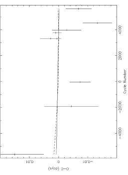
Figure 6: The O-C diagram for AC211. The solid line shows the best linear fit and the dashed line shows the best quadratic fit.

Table 4: X-ray observations used to calculate the ephemeris.

Mid-Eclipse	Error	Satellite/
(JD +2450000.0)	(days)	Instrument
43469.375877	0.009982	EXOSAT
46120.361216	0.009269	EXOSAT
47457.268883	0.003565	Ginga
49855.162059	0.003565	ASCA/GIS
49855.159920	0.001426	ASCA/SIS
50178.158	0.001	RXTE/PCA
50178.870	0.001	RXTE/PCA
50329.314230	0.004991	RXTE/ASM
50714.333947	0.004991	RXTE/ASM
51498.6614	0.0044	BeppoSAX

The low mass-loss rate estimates calculated from the Civ P-Cygni profile are in direct contrast with the large mass-loss rate calculated by Homer & Charles (1998). Their extremely high mass-loss rate was based on their conclusion that AC211 has a large period derivative. This prompted us to re-investigate the ephemeris question. We combined the original eclipse timings of Homer & Charles (1998) with additional X-ray observations (Paper I) and recalculated the ephemeris of AC211. We based our ephemeris calculation solely on the X-ray eclipse timings and we removed the optical CCD points that were originally used by Homer & Charles. However, we emphasize that it is the addition of the new X-ray points and not the exclusion of the CCD optical points, which is responsible for the difference between the two ephemerides. Table 4 lists all the points used in our ephemeris calculation. We found that the data could be folded on the following linear ephemeris, with the uncertainty in the last figure shown in brackets.

$$T_{0}=HJD\leavevmode\nobreak\ 2447484.371(5)+0.71301(2){\times}E$$ (2)

The above ephemeris is in very good agreement with the ephemeris of Ilovaisky et al. (1993). Our ephemeris residuals (O-C values) are shown in Fig.6. We also attempted a quadratic fit to the data. The best quadratic fit found corresponds to the following ephemeris (in days).

$$O-C=1.4{\times}10^{-4}-1.3{\times}10^{-7}E+2.3{\times}10^{-11}{\times}E^{2}$$ (3)

However, the above quadratic term is significant only at the 7% level! Thus our expanded data set provides no statistically-significant evidence for a period change in AC211.

8 Which lines are interstellar?

Apart from AC211 the STIS MAMA detector recorded the spectra of a number of other field stars. Comparing AC211 with the brightest other star on each visit, we can make a selection of which lines are due to the interstellar medium and which are intrinsic to AC211. We find that apart from the Heii, Civ, Siiv and Nv lines all the other lines which are present in AC211 are also present in the spectra of the two other field stars. The profiles of Siii, Feii and Alii are narrow profile, which is indicative of interstellar lines. However, Ly${\alpha}$, as well as the absorption features at 1261Å (Siii or Sii), 1303Å (Oi and Siiii blend) and 1336Å (Cii) have a broader profile in AC211 than in the spectra of the background field stars. This indicates that some of the absorption seen in these lines is intrinsic to AC211; indeed the Ly${\alpha}$ profile varies with phase.

Since the Siii absorption line at 1528Å shows none of these problems, we can use it to estimate the column of Si towards AC211. Savage & Sembach (1991) show that the apparent column density per unit velocity is given by:

$$N_{a}=\frac{3.768{\times}10^{14}}{f{\lambda}}{\int}ln\left[\frac{I_{0}(u)}{I(u)}\right]du$$ (4)

where $f$ is the absorption oscillator strength of the line, ${\lambda}$ is the wavelength in Å and $I_{0}(u),I(u)$ are the unabsorbed and absorbed line intensities respectively. $N$ is given here in units of atoms cm^-2 km s^-1. Savage & Sembach (1991) also show that apparent column densities calculated in this fashion are instrumentally blurred but non-the-less accurate as long as the line is resolved or unless the integration in Eq. 4 is performed over an entire line which has no saturated components. Normalizing our absorption profile to the continuum level and using an oscillator strength value for Siii of $f=0.2303$ (Morton, 1991), we calculate a value for $N_{Si}=(1.4{\pm}0.1){\times}10^{15}$cm^-2 towards AC211.

Shull & van Steenberg (1985) calculated galactic interstellar abundances using IUE for 244 early type stars for which a number of them (68) are halo objects. Of these, 25 lie in the direction of M15 ($l$=65, $b$=-27). Plotting the $log(N_{Si})$ against the $log(N_{H})$ values of the 25 stars and by fitting a straight line through the points we determine a value of $N_{H}=(3.5{\pm}0.2){\times}10^{20}$cm^-2. This is in excellent agreement with the $N_{H}$ value calculated in Paper I using an interstellar reddening value of $E_{(B-V)}=0.05$ from Djorgovski & Meylan (1993).

Using the same method, we have also measured the silicon and hydrogen column densities by for two other stars, whose spectra were also recorded on the MAMA CCD detector (the brightest, aside from AC211, on each visit). All the equivalent widths and derived column densities are given in Table 5.

Table 5: Column densities for Silicon and Hydrogen as derived by using the Siii 1528Å line.

Star	$W_{\lambda}$	$N_{Si}({\times}10^{15})$	$N_{H}({\times}10^{20})$
	(Å)	cm-2	cm-2
AC211	$0.89{\pm}0.06$	$1.4{\pm}0.1$	$3.5{\pm}0.2$
Star 1	$0.89{\pm}0.14^{a}$	$1.6{\pm}0.1$	$4.1{\pm}0.3$
Star 2	$0.88{\pm}0.22^{a}$	$0.89{\pm}0.14$	$1.8{\pm}0.4$

^a The equivalent width is measured from the mean weighted spectrum of the star.

9 Discussion

The HST STIS observations show that AC211 has a strong UV continuum with a host of absorption lines, many of which are interstellar in origin (Sect. 3 and 8). In addition there is a highly variable emission from Heii and a Civ P-Cygni profile (Sect. 5 and 6). Since the Heii line is uneclipsed, we conclude it must come from a relatively large volume above and below the disc (Sect. 5). From the Civ line we can estimate the mass-loss from the system as $\sim 10^{-11}$M_⊙ yr^-1 (Sect. 6) much lower than that suggested by the orbital period derivative of Homer & Charles (1998). However, the inclusion of new data implies the period derivative is no longer significant, and thus that the derived mass-loss rate is probably correct (Sect. 7). These facts all fit nicely within the normal expectation for an X-ray binary. To progress further, we must accept that AC211 is a high inclination eclipsing system, in which the X-ray source is hidden behind the rim of the accretion disc, and that the X-rays originate from an accretion disc corona. This has long been the standard model for AC211, albeit with problems. The discovery of M15 X-2 removes the major objection to this model, which is how such a system could show an X-ray burst (see, for example, the discussion in Paper 1). The simplest assumption now is that M15 X-2 was responsible for the burst, and that the compact object in AC211 is indeed hidden.

At first sight the eclipses seem to fit easily into this model. The optical eclipse is wide, as one would expect from the eclipse of an accretion disc, since the entire disc will be X-ray heated to temperatures which emit significant radiation in the optical. The UV eclipse is narrower, again expected as only the inner regions of the accretion disc emit significant UV light. Finally, the X-ray eclipse is wide, since it is again of an extended object, the corona. We note in passing that the flux at the bottom of the X-ray eclipse is consistent with that from X-2, i.e. it could well be that the eclipse of AC211 is total. Although this means the accretion disc corona is smaller than previously thought, it does not mean the X-ray source is point like. If it were, the eclipse ingress and egress would be vertical, instead their slopes imply the X-ray emitting region is similar in size to the secondary star.

The problem with the UV eclipse is twofold. First, it is not total; one would expect a small, compact UV region to be totally eclipsed. This is backed up by the fact that the UV ingress and egress is not vertical, but our poor phase coverage make this result uncertain. Second, one might not expect to see the inner disc at all; it should be hidden behind the disc rim. Thus it appears that the UV emitting region is significantly extended, but how, or why remains unclear. The only way around this conundrum would be to invoke variability, since the X-ray, optical and UV eclipses are not simultaneous. Such a solution is is unsatisfactory, though, since the X-ray and optical eclipses are relatively stable in width (Paper I and Ilovaisky et al., 1993), and the phases in common between our two HST visits are give similar UV fluxes.

10 Conclusions

The STIS UV observations presented here have shown that, although the eclipse in AC211 implies that the UV source is more centrally concentrated than either the X-ray or the optical source, it cannot be explained by a simple disc model.

The interstellar UV lines imply an $N_{H}=3.5{\pm}0.2{\times}10^{20}$ cm^-2, whilst the Civ P Cygni profile implies a mass-loss rate of Ṁ${}_{L}{\sim}1{\times}10^{-11}$M_⊙ yr^-1. This is at variance with the mass-loss rates implied by Homer & Charles (1998), but the addition of new X-ray data to the ephemeris calculation removes the need for a large period change, which in turned implied the high mass-loss rate.