The Spatial, Ionization, and Kinematic Conditions of the $z=1.39$ Damped Ly$\alpha$ Absorber in Q$0957+561$ A,B

Abstract

We examined the kinematics, ionization conditions, and physical size of the absorption clouds in a $z=1.3911$ damped Ly$\alpha$ absorber (DLA) in the double image lensed quasar Q $0957+561$ A,B (separation $135h_{75}^{-1}$ pc at the absorber redshift). Using HIRES/Keck spectra (FWHM$~{}\simeq 6.6$ km s^-1), we studied the Mgii $\lambda\lambda 2796,2803$ doublet, Feii multiplet, and Mgi $\lambda 2853$ transition in absorption. Based upon the Feii profiles (the Mgii suffers from saturation), we defined six “clouds” in the system of sightline A and seven clouds in system of sightline B. An examination of the $N(v)$ profiles, using the apparent optical depth method, reveals no clear physical connection between the clouds in A and those in B. The observed column density ratios of all clouds is $\log N({\hbox{{\rm Mg}\kern 1.00006pt{\sc i}}})/N({\hbox{{\rm Fe}\kern 1.00006pt{\sc ii}}})\simeq-2$ across the full $\sim 300$ km s^-1 velocity range in both systems and also spatially (in both sightlines). This is a remarkable uniformity not seen in Lyman limit systems. The uniformity of the cloud properties suggests that the multiple clouds are not part of a “halo”. Based upon photoionization modeling, using the $N({\hbox{{\rm Mg}\kern 1.00006pt{\sc i}}})/N({\hbox{{\rm Fe}\kern 1.00006pt{\sc ii}}})$ ratio in each cloud, we constrain the ionization parameters in the range $-6.2\leq\log U\leq-5.1$, where the range brackets known abundance ratio and dust depletion patterns. The inferred cloud properties are densities of $2\leq n_{\rm H}\leq 20$ cm^-3, and line of sight sizes of $1\leq D\leq 25$ pc. The masses of the clouds in system A are $10\leq M/M_{\odot}\leq 1000$ and in system B are $1\leq M/M_{\odot}\leq 60$ for spherical clouds. For planar clouds, the upper limits are $400h_{75}^{-2}$ M_⊙ and $160h_{75}^{-2}$ M_⊙ for A and B, respectively. We favor a model of the absorber in which the DLA region itself is a single cloud in this complex, which could be a parcel of gas in a galactic ISM. We cannot discern if the Hi in this DLA cloud is in a single, cold phase or in cold+warm phases. A spherical cloud of $\sim 10$ pc would be limited to one of the sightlines (A) and imply a covering factor less than 0.1 for the DLA complex. We infer that the DLA cloud properties are consistent with those of lower density, cold clouds in the Galactic interstellar medium.

1 Introduction

Damped Ly$\alpha$ absorbers (DLAs) are well appreciated as useful astronomical laboratories for measuring metal enrichment, nucleosynthetic processing, and dust evolution from $z=4$ to the present epoch (e.g. Pettini et al., 1994; Lu et al., 1996; Pettini et al., 1997; Vlaldilo, 1998; Pettini et al., 1999; Prochaska & Wolfe, 2000; Prochaska, 2002; Ledoux, Bergeron, & Petitjean, 2002). Their redshift number density evolution (Wolfe et al., 1995; Storrie–Lombardi et al., 1996; Rao & Turnshek, 2000) places constraints on $\Omega({\hbox{{\rm H}\kern 1.00006pt{\sc i}}},z)$, and probes the Hi mass function for column densities greater than $N({\hbox{{\rm H}\kern 1.00006pt{\sc i}}})=2\times 10^{20}$ cm^-2. The gas kinematics measured from low–ionization metal absorption lines in DLAs provides valuable data upon which hypotheses for their dynamical formation, evolution, and physical nature can be based. To date, these competing hypotheses include thick rotating disks (Prochaska & Wolfe, 1997, 1998), merging cold dark matter halos (Haehnelt, Steinmetz, & Rauch, 1998; McDonald & Miralda–Escudé, 1999), and supernovae winds (Nulsen, Barcon, & Fabian, 1998; Shaye, 2001, however, see Bond et al. 2001).

The fact that DLAs provide leverage on questions relating to cosmological chemical evolution, nucleosynthetic and dust evolution, galaxy and/or hierarchical clustering evolution, and global star formation evolution makes them one of the most useful, and therefore, important astronomical objects of study. Of the great deal that has been learned about DLAs, one property remains elusive; there is little direct observational evidence from which the characteristic size of the DLA “region” itself can be deduced. By DLA region, we mean the parcel of gas that is associated with the very large Hi column density greater than $N({\hbox{{\rm H}\kern 1.00006pt{\sc i}}})=2\times 10^{20}$ cm^-2. From the size estimates, one could then deduce the covering factor of DLAs within their host objects, as well as their densities, and most importantly, their masses (though this quantity is geometry dependent).

Associating DLAs with the normal, bright galaxy population and assuming a unity covering factor, Steidel (1993) deduced a characteristic size of $\sim 20h^{-1}_{75}$ kpc. However, it is now known that DLAs are associated with galaxies having a wide variety of morphological types, including $0.1~{}L^{\ast}$ galaxies and low surface brightness (LSB) galaxies (Le Brun et al., 1997; Rao & Turnshek, 1998; Bowen, Tripp, & Jenkins, 2001). Indeed, the luminous host of many DLAs remain undetected even after dedicated searches to find their diffuse Ly$\alpha$ emission (e.g., Deharveng, Bowyer, & Buat, 1990; Lowenthal et al., 1995), their optical continuum emission (e.g., Steidel et al., 1997; Kulkarni et al., 2000, 2001) and their H$\alpha$ emission (e.g., Bunker et al., 1999; Bouché et al., 2000; Kulkarni et al., 2000, 2001).

In the absence of a well–defined luminosity function for the luminous hosts of DLAs, and without knowledge of the covering factor of the DLA region in these objects, we remain ignorant of a characteristic DLA size. It is safe to say, however, that estimates incorporating low surface brightness galaxies in the luminosity function of known DLA hosts would drive down the characteristic size. Scaling the Steidel estimate by the ratio of $\Phi_{\ast}$ for the luminosity functions of normal bright galaxies (Lilly et al., 1995; Ellis et al., 1996; Lin et al., 1999) and LSB galaxies (e.g., Dalcanton et al., 1997), we find an approximate characteristic size of $(0.033/(0.033+0.08)\cdot 20h^{-1}_{75}\sim 6h_{75}^{-1}$ kpc.

The data directly constraining the physical sizes of DLAs are few. In the lensed quasar HE $1104-1805$, Smette et al. (1995) placed limits of $5$–$17h^{-1}_{75}$ kpc on a DLA in one of the images. A more constraining result was obtained by Michalitsianos et al. (1997), who used the lensed quasar Q $0957+561$ A,B to show that the physical extent of a DLA at $z=1.3911$ is less than $135h_{75}^{-1}$ pc. On the other hand, Petitjean et al. (2000) suggest a lower limit of $200h_{75}^{-1}$ pc for a probable DLA in the lensed quasar APM $08279+5255$ (based upon partial covering arguments). Using VLBA observations of the slightly extended radio quasar B $0738+313$, Lane, Briggs, & Smette (2000) find $\log N({\hbox{{\rm H}\kern 1.00006pt{\sc i}}})=21.2$ cm^-2 in 21–cm absorption at two locations separated by $20h^{-1}_{75}$ pc [we note, however, that 21–cm emission line techniques may not be selecting objects that are one and the same as the DLAs selected using quasar absorption line techniques (see Rao & Turnshek, 2000; Churchill, 2001)].

In addition to the great insights garnished from low– to moderate–resolution spectroscopic studies of multiply imaged quasars, high resolution spectra provide constraints on the kinematics of metal–line systems at the few kilometers per second level (e.g., Rauch, Sargent, & Barlow, 1999; Lopez et al., 1999; Petitjean et al., 2000; Rauch et al., 2002b). This means the gaseous structure can be studied component by component, directly providing their sightline to sightline velocity shears, $\Delta v/\Delta r$, where $r$ is the physical separation of the sightlines at the absorber. Such measurements allow insights into the ionization structures, masses, density gradients, and energy input budgets (e.g., Rauch, Sargent, & Barlow, 1999; Rauch et al., 2002a; D́Odorico, Petitjean, & Christiani, 2002). It is important to realize that these insights are derived based upon models of the gas dynamics and geometry. These models, however, are strongly founded upon observations of the gaseous components in the Milky Way, LMC, SMC, and other local galaxies.

The reasonably bright gravitationally lensed quasar Q $0957+561$ A,B at $z_{em}=1.41$ with separation 6″ provides an excellent opportunity to study high–resolution spectra of two sightlines through a $z>1$ DLA (e.g., Walsh, Carswell, & Weymann, 1979; Wills & Wills, 1980; Young et al., 1980, 1981a, 1981b; Turnshek & Bohlin, 1993; Michalitsianos et al., 1997; Zuo et al., 1997; Pettini et al., 1999). The $z=1.3911$ absorber has a neutral hydrogen column density of $N({\hbox{{\rm H}\kern 1.00006pt{\sc i}}})=1.9\pm 0.3\times 10^{20}$ cm^-2 in the A spectrum and $N({\hbox{{\rm H}\kern 1.00006pt{\sc i}}})=8\pm 2\times 10^{19}$ cm^-2 in the B spectrum (Zuo et al., 1997). This suggests that the DLA region is concentrated in front of the A image. At the redshift of the absorber, the physical separation of the A and B sightlines is $135h_{75}^{-1}$ pc (Smette et al., 1992). Zuo et al. (1997) found a differential reddening in spectrum A as compared to spectrum B and deduce a dust to gas ratio of $\sim 0.6$ in the DLA. Imaging of the quasar field has been reported by Dalhe, Maddox, & Lilje (1994, ground based) and Bernstein et al. (1997, WFPC2/HST). Despite these efforts, the luminous object associated with the $z=1.3911$ absorber remains unidentified.

The most extensive study of the DLA to date, using FOS/HST spectra ($R=1300$), was presented by Michalitsianos et al. (1997). In general, they found “the differences in the damped Lyman series absorption in the lensed components are the only significant spectral characteristics that distinguishes the far–ultraviolet spectra of Q $0957+561$ A,B.” Assuming a spherical geometry and a neutral hydrogen fraction of $N({\hbox{{\rm H}\kern 1.00006pt{\sc i}}})/N({\rm H})=0.05$ (Chartas et al., 1995), the authors estimate the DLA mass to be $2.6\times 10^{6}$ M_⊙, which they interpreted to be consistent with a giant molecular cloud or a small condensation (spiral arm) within a galactic disk (viewed pole on). Because the metal lines are tightly correlated for the two sightlines, Michalitsianos et al. (1997) suggested that the large metal–line absorption arises in a galactic “halo”.

In this paper, we present $R=45,000$ HIRES/Keck spectra of the Q $0957+561$ A,B. We focus on the Mgii $\lambda\lambda 2796,2803$ doublet, the Mgi $\lambda 2853$ transition, and several Feii transitions arising in the DLA at $z=1.3911$. In § 2, we present the data, and briefly describe the data reduction and analysis. We present the observed kinematic and spatial properties of the absorber column densities in § 3. Assuming photoionization equilibrium, we model the clouds and present their densities, sizes, and masses in § 4. We briefly discuss these properties in § 5 and provide concluding remarks in § 6.

2 The Data

The lensed quasar Q $0957+561$ A,B was observed on the nights of 1994 November 26–27 with the HIRES instrument (Vogt et al., 1994) on the Keck–I telescope. HIRES was configured in first order using decker C1 (7″ in the spatial 0.861″ in the dispersion directions, respectively). The resolution of $R=45,000$ corresponds to a velocity resolution of ${\rm FWHM}=6.6$ km s^-1. The resulting observed wavelength range is 4600 to 6900 Å. As such, many different transitions were covered; however, we detected only the Mgii $\lambda\lambda 2796,2803$ doublet, the Feii $\lambda$2344, 2374, 2383, 2587, & 2600 multiplet, and the Mgi $\lambda 2853$ transition.

The quasar images A and B were observed individually. Three 1500 second exposures were obtained for each image. The resulting spectra have signal–to–noise ratios of $\simeq 30$ per resolution element. The individual spectra were reduced and calibrated using the IRAF Apextract package for echelle data. The wavelength scale is vacuum and has been corrected to the heliocentric velocity. Continuum normalization was performed as described in Sembach & Savage (1992) and Churchill (1997).

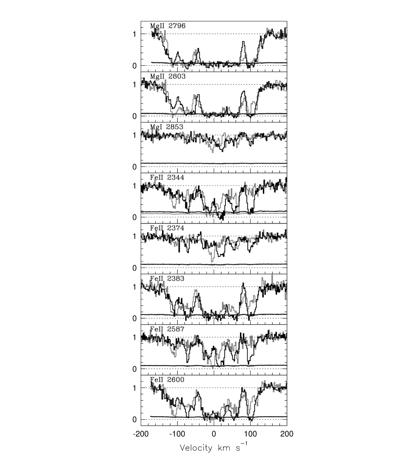
Figure 1: Normalized HIRES/Keck spectra of the Mgii, Mgi, and Feii absorption profiles presented in the system rest–frame velocity. A spectra are black and B spectra are grey. The velocity zero point is set to $z=1.390861$, which is the optical depth mean of the Mgii $\lambda 2796$ transition in the A spectrum.

In Figure 1, we present the observed Mgii, Mgi, and Feii absorption profiles for the $z=1.391$ absorber as a function of rest–frame velocity, where the A spectra (black) and B spectra (grey) are over plotted on the same velocity scale. The velocity zero point is set to $z=1.390861$, which corresponds to the optical depth mean of the Mgii $\lambda 2796$ profile for the system in sightline A (see Appendix A.1 of Churchill & Vogt, 2001).

3 Column Densities and Kinematics

We modeled the data using Voigt profile (VP) decomposition. The fitting was performed with the code MINFIT (Churchill, 1997; Churchill, Vogt, & Charlton, 2002). The VP models provide the number of clouds and their velocities, column densities, and Doppler parameters. Because VP analysis is non–unique (especially in highly saturated profiles), and because it is sensitive to the signal–to–noise ratio and resolution of the spectra (Churchill, 1997; Churchill, Vogt, & Charlton, 2002), we use the VP parameters as a secondary means of studying the column densities and kinematics. Instead, we use the apparent optical depth method (Savage & Sembach, 1991) as the primary means of studying the relationship between cloud velocities and column densities.

3.1 Apparent Optical Depth Method

Apparent column densities per unit velocity, $N_{a}(v)$ [atoms cm^-2/(km s^-1)], were measured for each transition using the formalism described by Savage & Sembach (1991). These column density spectra and their uncertainty spectra were then linearized to a common velocity binning of 2.23 km s^-1 using flux conservation. From these linearized data, an optimal column density was computed for each species in each velocity bin. The algorithm employed for computing optimal column densities has been described in Appendix A.5 of Churchill & Vogt (2001).

In brief, for adoption of the optimal $N_{a}(v)$ for an ion we employ one of three possibilities: (1) All transitions of an ion exhibit some saturation between $v_{b}$ and $v_{r}$, so that $N_{a}(v)$ is a lower limit. Often, the transition with the smallest $f\lambda$ provides the best constraints on the lower limit; (2) All but one transition of an ion exhibits saturation, in which case, the adopted column density is taken from the unsaturated transition; and (3) All or more than one transition of an ion are unsaturated, providing multiple independent measurements. The optimal $N_{a}(v)$ is computed from the weighted mean in each velocity bin.

The Mgii transitions in both systems exhibited unresolved saturation across the majority of the profiles and therefore provide only upper limits on $N_{a}(v)$ at most velocities. Though the stronger Feii transitions ($\lambda 2383$ and $\lambda 2600$) exhibited saturation over the velocity intervals $(-30,+30)$, $(+50,+70)$, and $(+90,+110)$, the weakest transition ($\lambda 2374$), and to a lesser extent the $\lambda 2587$ transition, provide a robust $N_{a}(v)$ across these intervals. Mgi has no velocity regions with unresolved saturation.

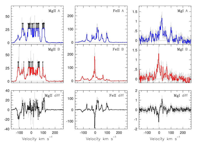
Figure 2: The optimal apparent column densities profiles, $N(v)$, for Mgii (left), Feii (center), and Mgi (right) presented in the system rest–frame velocity. The grey shading is the $1~{}\sigma$ uncertainties in the $N(v)$ profiles. The lower panels show the differences A$-$B.

In Figure 2, we present $N(v)$, the optimal apparent column densities, for Mgii (left), Feii (center), and Mgi (right) as a function of rest–frame velocity. The upper panels show $N(v)$ for systems of sightlines A and B (hereafter, systems A and B) as labeled and the lower panels show the column density difference, $\Delta N(v)=N_{A}(v)-N_{B}(v)$. Limits are represented by arrows and $1~{}\sigma$ uncertainties are shown as grey shading.

A prominent feature of the data in Figure 2, is the $N(v)$ peak for Feii and Mgi in system A at $v\simeq+20$ km s^-1. A second, even more prominent $N(v)$ peak is at $v\simeq-10$ km s^-1 in system B. Interestingly, for Feii, the difference profile, $\Delta N(v)$, reveals positive (A$>$B) and negative (A$<$B) peaks with a quasi–periodicity of $\simeq 40$ km s^-1. In some cases these $\Delta N(v)$ peaks are due to different strengths of $N(v)$ peaks aligned in velocity in both systems. In other cases the $\Delta N(v)$ peaks are due to the presence of an $N(v)$ peak in the one system and the lack of an $N(v)$ peak in the other at the same velocity.

3.2 Velocity Correlations

A striking feature of the data is the velocity alignment of an absence of absorption at $v\simeq+80$ km s^-1, as can be clearly seen in the Mgii and strongest Feii profiles in Figure 1. This may indicate that the parcel of gas giving rise to absorption at $v\simeq+100$ km s^-1 is a separate physical entity from that giving rise to the lower velocity absorption. If so, this gas has little to no velocity sheer across the sightlines. At $v\simeq-50$ km s^-1 and at $v\simeq-100$ km s^-1 there are similar, yet less pronounced, profile inversions. In this case, there is a small difference of $\sim 20$ km s^-1, which translates to a velocity sheer of $0.15h_{75}$ km s^-1 pc^-1. Again, this could indicate that the higher (negative) velocity gas is physically distinct from the lower velocity gas.

Ultimately, it is difficult to extract physical information directly from the flux values of such strong absorption lines, which exhibit saturation over much of the velocity interval. In order to further study the cloud–by–cloud kinematic connections between systems A and B, we ran a cross–correlation on the Feii and Mgi $N(v)$ profiles. The cross–correlation function is defined by

$$\xi(\Delta v)=\frac{\sum\left[N_{A}(v)-\left<N_{A}\right>\right]\cdot\left[N_{B}(v-\Delta v)-\left<N_{B}\right>\right]}{\sqrt{\sum\left[N_{A}(v)-\left<N_{A}\right>\right]^{2}\cdot\sum\left[N_{B}(v-\Delta v)-\left<N_{B}\right>\right]^{2}}},$$ (1)

where $\Delta v$ is the lag velocity between the two systems. Equation 1 is defined so that a perfect correlation is $\xi=+1$ and no correlation is $\xi=0$ In Figure 3, we present $\xi$ as a function of $\Delta v$. The left hand panels are Feii and the right hand panels are Mgi. The top (middle) panels show the self–correlation function for system A (B). By definition, these functions are symmetric about the lag velocity and have unity at zero lag velocity.

The $\xi$ for Feii in system A shows a remarkable pattern; there is a $40$ km s^-1 periodicity in the clouds, as evident in the two peaks in $\xi$ at $\left|\Delta v\right|\simeq 40$ and $80$ km s^-1. There is a lack of periodicity in the Feii for system B; the cross–correlation function reveals the velocity difference of the two strongest clouds separated by $\Delta v\simeq 80$ km s^-1. The clouds in system A, in general, have large $N$, so it is quite clear that this periodicity in system A is driving the shape of the $\Delta N(v)$ profile shown in Figure 2.

The $\xi$ for Mgi shows no periodicity, but only the velocity differences between the strongest components. Note the “noise” in $\xi$ for system B Mgi at $30\leq\left|\Delta v\right|\leq 60$ km s^-1, which has a magnitude of $\delta\xi\simeq 0.1$; this arises in the noisiest data and provides an estimate of the significance level of the stronger peaks for all of the cross–correlation functions.

In the lower panels of Figure 3, we show the cross–correlation functions for system A against system B. The peaks in these functions provide the velocity difference between the strongest components in each system, which lies at $\Delta v\simeq-27$ km s^-1 for both Feii and Mgi. A peak of $\xi\simeq 0.7$ is significantly below unity (approximately $3~{}\sigma$, based upon the above noise estimates) and quantifies the level at which the two Feii profiles do not resemble each other kinematically; $\xi$ is dominated by the strongest components in complex profiles.

Overall, this exercise reveals that there is no clear signal in the cross–correlation function for similar kinematics in the system A and system B profiles. This indicates that the clouds are not clearly traceable between the two sightlines.

3.3 Integrated Column Densities

In Table 1, we present the integrated apparent column densities, $N$, for the Mgii, Feii and Mgi ions. The $N$ were computed for fixed velocity intervals (from $v_{1}$ to $v_{2}$) using the data presented in Figure 2. The velocity intervals were defined by local $N(v)$ minima in the Feii spectra for system A and B individually. Six velocity intervals were found for system A and seven were found for system B. These intervals roughly represent individual “clouds” giving rise to the complex absorption profiles.

As stated above, the Mgii transitions provide only upper limits for most velocity intervals. The exception is velocity interval 1 (or “cloud number 1”) in system A. Clouds 2, 3, 5, and 7 in systems B are marginally saturated; there is at least one saturated pixel in each of these clouds. For this reason, we quote these particular clouds in system B as upper limits. However, unless there are high column density clouds with $b\leq 2$ km s^-1 at the location of these saturated pixels, the quoted values for system B could be marginally acceptable as measurements. We choose to not invoke them as measurements for our analysis.

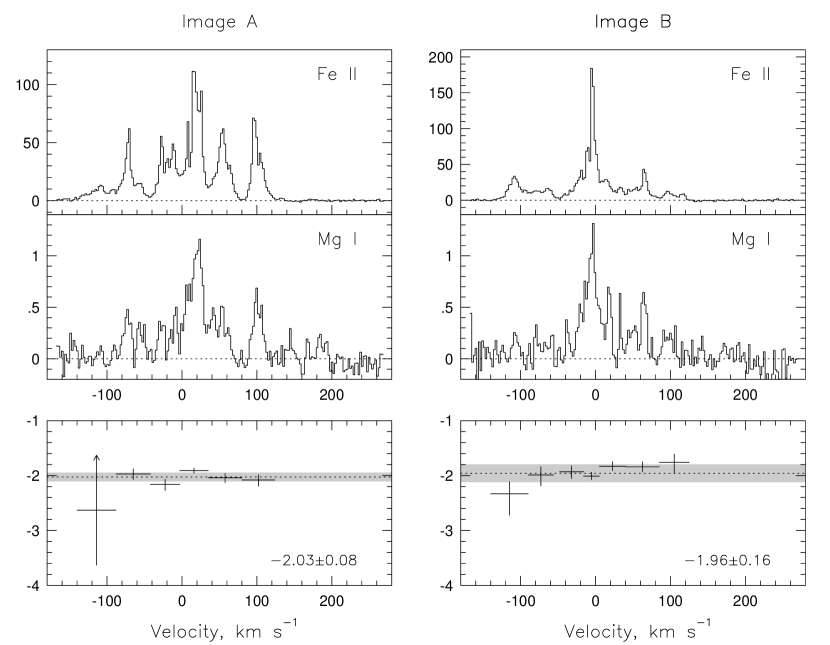
Figure 4: The optimal apparent column densities profiles, $N(v)$, for Feii and Mgi presented in the system rest–frame velocity. A spectra are on the left and B spectra on the right. The bottom panels show the ratios of the integrated column densities for each of the velocity bins corresponding to “separate clouds” in the Feii profiles. The dotted horizontal line is the average of the individual clouds and the grey shaded area is the standard deviation. This average and standard deviation are written in the corner of the respective panels.

For both systems, we computed the column density ratios $N({\hbox{{\rm Mg}\kern 1.00006pt{\sc i}}})/N({\hbox{{\rm Fe}\kern 1.00006pt{\sc ii}}})$ for each cloud and listed them in Table 1. The $N({\hbox{{\rm Mg}\kern 1.00006pt{\sc i}}})/N({\hbox{{\rm Fe}\kern 1.00006pt{\sc ii}}})$ data are plotted in Figure 4. The horizontal bars of the data points give the velocity interval of the $N(v)$ integrations and the vertical bars give the uncertainties in the column density ratio. Plotted in the upper panels of Figure 4, and aligned in velocity space for ease of inspection, are the Feii and Mgi $N(v)$ profiles.

As seen in Figure 4, the ratios for all clouds in both systems A and B are consistent with $\log N({\hbox{{\rm Mg}\kern 1.00006pt{\sc i}}})/N({\hbox{{\rm Fe}\kern 1.00006pt{\sc ii}}})\simeq-2$. This result suggests a high level of uniformity in both the gas–phase [Mg/Fe] abundance patterns and ionization conditions across velocity space.

The VP subcomponents describing these dominant “clouds” also have ratios relatively consistent with these findings, with $-2.02\pm 0.04$ in system A and $-2.1\pm 0.3$ in system B.

Integration of $N(v)$ across the full profiles yields $\log N({\hbox{{\rm Mg}\kern 1.00006pt{\sc i}}})/N({\hbox{{\rm Fe}\kern 1.00006pt{\sc ii}}})=-2.03_{-0.08}^{+0.07}$ for system A and $-1.96_{-0.15}^{+0.16}$ for system B. These quantities are shown as grey shaded regions on Figure 4. The individual clouds have ratios that are consistent with that of the full system. This level of uniformity with velocity is consistent with that reported by Prochaska (2002) for a sample of 13 higher redshift DLAs. Worth noting is that these data also provide direct evidence of spatial uniformity on the scale of $135h^{-1}_{75}$ pc in a DLA.

4 Nature of the Absorbers

4.1 Photoionization Modeling

Inferring the physical conditions in the clouds is model dependent. Here, we assume photoionization equilibrium. Using the measured column densities as constraints on the models, we derive the cloud metallicities, densities, sizes, and masses.

We used Cloudy (Ferland, 1998) to construct grids of model clouds. We assume that the $N({\hbox{{\rm H}\kern 1.00006pt{\sc i}}})$ in system A clouds is $\log N=20.3$ cm^-2 and in system B clouds is $\log N=19.9$ cm^-2 (Zuo et al., 1997). Since the measured $N({\hbox{{\rm H}\kern 1.00006pt{\sc i}}})$ is actually the sum of individual clouds in a system, we note that some inferred properties (sizes and masses) for the individual clouds will be overestimated.

Each cloud is modeled as a constant density plane–parallel “slab” with ionizing radiation incident on one face. For the ionizing flux, we used the $z=1.4$ ultraviolet background (UVB) spectrum of Haardt & Madau (1996) and Madau, Haardt, & Rees (1999). The separation velocity of the DLA and the quasar is $\simeq 2500$ km s^-1. Thus, it could be argued that the absorber is not an intervening system, but is associated with the quasar itself. If so, the quasar flux, and not the UVB flux, would dominate the photoionization of the gas.

One indicator of associated absorption is the presence of partial covering (Barlow & Sargent, 1997; Hamman, 1997; Ganguly et al., 1999). None of the low ionization transitions we observed show signs of partial covering. That is to say, that the fully saturated regions of the Mgii $\lambda\lambda 2796,2803$ doublet members are black (statistically consistent with zero flux) in their cores. Also, at the same velocity intervals where Feii $\lambda 2383$ and $\lambda 2600$ are also fully saturated, their absorption is also black. As such, we assume that the DLA is intervening. If the absorber is intervening, then the cosmological separation ($\Delta z=0.02$) from the quasar is $\sim 15h^{-1}_{75}$ Mpc. It has been argued that, at this distance, the quasar flux does not affect the ionization balance in the absorber (Michalitsianos et al., 1997).

At $h\nu=13$ eV, the flux normalization is $\nu F_{\nu}=1.26\times 10^{-5}$ erg s^-1 cm^-2. We output the column densities for selected ionic species (esp. Mgii, Mgi, and Feii) as a function of ionization parameter, $U=n_{\gamma}/n_{\rm H}$. This quantity is the ratio of the number density of photons capable of ionizing hydrogen to the number density of hydrogen atoms. We explored the range $-8\leq\log U\leq-1$ in 0.1 dex intervals.

For these large $N({\hbox{{\rm H}\kern 1.00006pt{\sc i}}})$ values, the model clouds are optically thick and have an extended neutral layer. As such, the relative dependence of the column densities with ionization parameter are indistinguishable between the $\log N=20.3$ cm^-2 and $\log N=19.9$ cm^-2 cloud models.

4.2 Metallicity

In Table 2, we list the $3~{}\sigma$ rest–frame equivalent widths of selected transitions. We infer upper limits on the cloud metallicities using the Znii $\lambda 2026$ transition, which only weakly depletes onto dust and is known to trace Fe–group elements (e.g., Savage & Sembach, 1996; Lauroesch et al., 1996). No Znii was detected in our spectra; the $3~{}\sigma$ equivalent width limit was $13$ mÅ in system A and $15$ mÅ in system B. Without detections of Crii and Znii we cannot directly estimate the effects of dust in these systems (see Zuo et al., 1997).

For these equivalent widths, Znii $\lambda 2026$ is effectively on the linear portion of the curve of growth. We obtain an upper limit of $\log N({\hbox{{\rm Zn}\kern 1.00006pt{\sc ii}}})<11.9$ cm^-2 for system A and $\log N({\hbox{{\rm Zn}\kern 1.00006pt{\sc ii}}})<12.0$ cm^-2. In the cloud models $N({\hbox{{\rm Zn}\kern 1.00006pt{\sc ii}}})$ is affectively independent of ionization parameter for $\log U<-3.5$ and decreases by only 0.5 dex from $\log U=-3.5$ to $-1$. For $\log U<-3.5$, we obtain an upper limit of [Zn/H]$<-1$ for system A and [Zn/H]$<-0.5$ for system B.

These values are corroborated by upper limits based upon the weaker Znii $\lambda 2063$ transition. Our HIRES/Keck spectra provide only slight improvements over the limits (also $3~{}\sigma$) of [Zn/H]$<-0.75$ for system A and [Zn/H]$<-0.31$ for system B reported by Pettini et al. (1999).

4.3 Ionization Parameter: A Matter of Dust

In the model clouds, $N({\hbox{{\rm Mg}\kern 1.00006pt{\sc ii}}})$ and $N({\hbox{{\rm Fe}\kern 1.00006pt{\sc ii}}})$ are virtually independent of $U$, whereas $N({\hbox{{\rm Mg}\kern 1.00006pt{\sc i}}})$ decreases about 0.8 dex for every 1 dex increase in $U$. The $N({\hbox{{\rm Mg}\kern 1.00006pt{\sc i}}})/N({\hbox{{\rm Mg}\kern 1.00006pt{\sc ii}}})$ ratio could provide an estimate of the cloud ionization parameters; however, the Mgii profiles are severely saturated. Since the $N(v)$ profiles for Feii are well defined at all velocities, the $N({\hbox{{\rm Mg}\kern 1.00006pt{\sc i}}})/N({\hbox{{\rm Fe}\kern 1.00006pt{\sc ii}}})$ ratio, in principle, holds potential for inferring the ionization parameter. In Figure 5, we show the Feii and Mgi column densities as a function of $\log U$ for one of our Cloudy models. This model cloud has $\log N({\hbox{{\rm H}\kern 1.00006pt{\sc i}}})=20.3$ cm^-2 and a solar abundance pattern. For presentation purposed, we have scaled the metallicity to $[Z/Z_{\odot}]=-2$ to match the integrated $N$ for system A presented in Table 1. The logarithm of the ratio $N({\hbox{{\rm Mg}\kern 1.00006pt{\sc i}}})/N({\hbox{{\rm Fe}\kern 1.00006pt{\sc ii}}})$ decreases from $\simeq-0.5$ at $\log U=-8$ to $\simeq-4.5$ at $\log U=-3$, after which it begins to decrease rapidly. For a solar abundance pattern and no dust depletion, the cloud models for both systems have $\log N({\hbox{{\rm Mg}\kern 1.00006pt{\sc i}}})/N({\hbox{{\rm Fe}\kern 1.00006pt{\sc ii}}})\simeq-2$ for $\log U\simeq-6$.

The fact of the matter, however, is that $N({\hbox{{\rm Mg}\kern 1.00006pt{\sc i}}})/N({\hbox{{\rm Fe}\kern 1.00006pt{\sc ii}}})$ is directly proportional to the gas–phase [Mg/Fe] abundance ratio, which can be strongly affected by the dust depletion factors for Mg and for Fe. The study of the effects of dust in DLAs is one of central importance (e.g., Ellison et al., 2001, and references therein).

Zuo et al. (1997) report a dust to gas ratio of $\sim 0.6$ for the $z=1.3911$ DLA studied here. However, we note that there are several assumptions invoked for their calculations, including extrapolation of the Galactic extinction law and no time delay or variability between the lensed images. The latter is certainly not strictly true ($\Delta\tau\simeq 420$ days, Kundić et al., 1997; Haarsma et al., 1999), and the former may not apply to DLAs (e.g., Pettini et al., 1997; Prochaska, 2002) even if the extrapolation accurately represents the Galactic law. Even without a definitive estimate of the dust content in this DLA, we can explore how dust depletion might effect the inferred cloud properties.

In the Galaxy, dust depletion factors for Mg range from $\delta=-0.3$ in warm “halo” gas to $\delta=-1.6$ in cool “disk” gas and for Fe range from $\delta=-0.6$ to $-2.3$ (Lauroesch et al., 1996; Savage & Sembach, 1996; Welty et al., 1999, 2001). In order to allow for the observed range in [Mg/Fe] due to dust depletion, we also consider cloud models with warm halo and cool disk dust depletion factors. These ranges also encompass the observed range of $\alpha$–group to Fe–group variations observed in the photosphere of Galactic stars (McWilliam et al., 1995; Lauroesch et al., 1996; Johnson, 2002), globular cluster stars (Smith et al., 2000; Stephens & Bosegaard, 2002), LMC/SMC stars (Venn, 1998), and dwarf galaxies (Shetrone, Côté, & Sargent, 2001).

For the warm halo pattern we find the lower limit of $\log U\simeq-6.2$ and for the cold disk pattern we find the upper limit of $\log U\simeq-5.1$; we have,

$$-6.2\leq\log U\leq-5.1$$ (2)

for both the system A and system B clouds, where the no–dust, solar abundance pattern value is $\log U=-6.0$.

We adopt this range in $\log U$ as an estimate of the inferred ionization condition in the clouds. We note, however, there is growing observational evidence that dust depletion in DLAs may not be significant and may be fairly uniform both from system to system (Pettini et al., 1999; Ellison et al., 2001) and from velocity component to velocity component within a system (Prochaska, 2002). However, we note that there are examples of possible intrinsic abundance variations of [Mn/Fe] in DLAs (Ledoux, Bergeron, & Petitjean, 2002) and of strong dust depletion in DLAs selected because they are strong molecular hydrogen absorbers (e.g., Petitjean, Srianand, & Ledoux, 2002).

The statistical data supporting low dust content in DLAs would suggest that the above range of ionization parameters serves as a somewhat conservative approach for bracketing the inferred ionization parameter. The largest uncertainty lurks in the original assumption that the clouds are in photoionization equilibrium.

4.4 Densities, Sizes, and Masses

For the UVB spectrum normalized at $z=1.4$, the relationship between the hydrogen number density of the clouds and the ionization parameter is

$$\log n_{\rm H}=-4.9-\log U~{}~{}{\rm cm}^{-3},$$ (3)

for constant density cloud models. For the inferred range of ionization parameters, we find

$$3\leq n_{{\rm H},A}\leq 20~{}~{}{\rm cm}^{-3},\quad{\rm and}\quad 2\leq n_{{\rm H},B}\leq 15~{}~{}{\rm cm}^{-3},$$ (4)

for the system A clouds and system B clouds, respectively. These densities fall within the lower density range for cold clouds in the Galactic interstellar medium (Spitzer, 1985; Savage & Sembach, 1996). The cloud line–of–sight physical extent, $D=N({\rm H})/n_{\rm H}$, is then,

$$\log D=\log N({\rm H})+\log U-13.7~{}~{}{\rm pc},$$ (5)

where $N({\rm H})$ is the total hydrogen column density. For the inferred range of ionization conditions, the ionization fraction of hydrogen is negligible so that the approximation $N({\rm H})=N({\hbox{{\rm H}\kern 1.00006pt{\sc i}}})$ holds. We obtain,

$$5\leq D_{A}\leq 25~{}~{}{\rm pc},\quad{\rm and}\quad 1\leq D_{B}\leq 15~{}~{}{\rm pc},$$ (6)

for the system A and system B clouds, respectively. To the extent that the photoionization modeling has provided a reasonable approximation of the cloud physical conditions, we can infer that the cloud sizes are roughly a factor of ten smaller than the sightline separation of the lensed quasar.

We can estimate the cloud mass under the assumption of spherical symmetry, which gives $M\propto m_{\rm H}n_{\rm H}(D/2)^{3}$, where $m_{\rm H}$ is the mass of hydrogen. In terms of our parameterizations, the cloud mass is,

$$\log M=3\log N_{\rm H}+2\log U-47.7~{}~{}{\rm M}_{\odot},$$ (7)

which alternatively can be written as

$$M\simeq 2N_{20}^{3}U_{-6}^{2}~{}~{}{\rm M}_{\odot},$$ (8)

where $N_{20}$ is the total hydrogen column density of the cloud in units of $10^{20}$ cm^-2, and $U_{-6}$ is the ionization parameter in units of $10^{-6}$. We find approximate masses of

$$10\leq M_{A}/M_{\odot}\leq 1000\quad{\rm and}\quad 0.5\leq M_{B}/M_{\odot}\leq 60,$$ (9)

for the system A and system B clouds, respectively, for the range of ionization parameters given in Equation 4.

If we instead assume that the clouds are cylindrical “slabs” with “height” $D=N({\rm H})/n_{\rm H}$ and “radius” $R$, we have $M\propto m_{\rm H}n_{\rm H}DR^{2}$, which can be simplified to

$$M\simeq 25N_{20}R_{100}^{2}~{}~{}{\rm M}_{\odot},$$ (10)

where $R_{100}$ is the cylinder radius in units of 100 pc. Note that the mass for this geometry is independent of the cloud density, $n_{\rm H}$, and therefore ionization parameter, $U$. Given that we cannot track the individual clouds from sightline A to sightline B, a conservative upper limit of $R_{100}=2h_{75}^{-1}$ can be applied. With this upper limit, we obtain

$$M_{A}\leq 400h_{75}^{-2}~{}~{}{\rm M}_{\odot}\quad{\rm and}\quad M_{B}\leq 160h_{75}^{-2}~{}~{}{\rm M}_{\odot},$$ (11)

for upper limits on the system A and system B cloud masses.

4.5 Caveats

We examined the effects on the above inferred cloud properties of different shapes of the ionizing spectrum. We examined a grid of Cloudy models in which O stars and B stars contributed to and/or dominated over the UVB. We followed the formalism of Churchill, Vogt, & Charlton (2002) and Churchill & Le Brun (1998) (esp., see Figures 12 and 13 of Churchill, Vogt, & Charlton (2002)). We find that the contribution of O and B stars makes virtually no difference in the inferred cloud properties. This is due to the high level of self–shielding in the clouds. Thus, we find that the inferred cloud properties are robust under the assumption of photoionization equilibrium.

It is important to point out that the above inferred sizes and masses are overestimates within the formalism we have utilized. Each individual cloud was assumed to have identical $N({\hbox{{\rm H}\kern 1.00006pt{\sc i}}})$, and the value applied was the total $N({\hbox{{\rm H}\kern 1.00006pt{\sc i}}})$ for each respective system. That is, all system A clouds were assumed to have $\log N({\hbox{{\rm H}\kern 1.00006pt{\sc i}}})=20.3$ cm^-2 and all system B clouds were assumed to have $\log N({\hbox{{\rm H}\kern 1.00006pt{\sc i}}})=19.9$ cm^-2. Therefore, the inferred sizes and masses for these clouds are smaller than we have quoted here.

5 Discussion

As first inferred from the FOS/HST spectra and confirmed here, the absorber appears to have a projected transverse physical extent no greater than $\simeq 135h^{-1}_{75}$ pc and seems to be enshrouded by an optically thick gaseous complex (Michalitsianos et al., 1997). We have resolved the kinematics of the low ionization gas in these systems and find the total velocity spread to be $\sim 300$ km s^-1, based upon the Mgii $\lambda\lambda 2796,2803$ doublet.

We have defined six “clouds” for system A and seven clouds for system B. The data and photoionization models suggest a picture in which the sightline physical extent (sizes) of the clouds in this DLA are of the order 10 pc. The inferred densities are $\sim 10$ cm^-3, and the masses are no greater than $\sim 400h_{75}^{-2}$ M_⊙. The temperatures of the cloud models, if they are taken at face value, have a gradient with values that range from $T\simeq 2000$ K at the cloud face to $T\simeq 500$ K at the cloud core. To the extent that the assumption of photoionization equilibrium is appropriate and has been modeled accurately, we have found that the DLA clouds are similar to low mass (10–100 M_⊙), low density (1–10 cm^-3), cold ($\sim 1000$ K) Hi clouds in the Milky Way (Spitzer, 1985; Savage & Sembach, 1996).

5.1 Where lies the DLA?

Directing our attention to the physical nature of DLAs, we focus on two questions. (1) Is the DLA region itself only one of these small clouds, and therefore does it exhibit very narrow kinematics? (2) Is the DLA region only a single phase of gas, or can it arise in a cold phase and a warm phase (e.g., Lane, Briggs, & Smette, 2000)? The answer to these questions will provide clues for interpreting the observed abundance ratio and ionization uniformity between the clouds.

Based upon the cross–correlation (see Equation 1) of the system A and system B profiles, we find that the individual Mgii and Feii clouds are not identifiable between the two sightlines separated by $135h^{-1}_{75}$ pc. This implies that we do not track the same clouds from sightline A to B, which in turn implies that they are smaller than the line of sight separation. Rauch et al. (2002b) found a similar lack of a clear identification between clouds in an optically thick Mgii absorber at $z=0.5656$ in the triple sightlines of Q $2237+0305$, which have separations of 135–200$h^{-1}_{75}$ pc.

However, the cross–correlation function has a single strong peak, indicating that there is a single strongest component in each system; system A has a strongest absorbing component at $v\simeq+20$ km s^-1, and system B has a dominant component at $v\simeq-10$ km s^-1 (see Figure 2). It is reasonable to argue that the DLA region is physically associated with the sites of strongest absorption. In numerical simulations of hierarchical clustering, the strongest absorption lines arise in the single most highly peaked baryon overdensities (e.g. Haehnelt, Steinmetz, & Rauch, 1996; Rauch, Haehnelt, & Steinmetz, 1997).

Because there are only low resolution spectra available for the neutral hydrogen lines (e.g. Turnshek & Bohlin, 1993; Michalitsianos et al., 1997; Zuo et al., 1997; Pettini et al., 1999), the measured $N({\hbox{{\rm H}\kern 1.00006pt{\sc i}}})$ contains no direct kinematic information. However, using the kinematics of the Feii gas as a template for the neutral hydrogen, we use the Ly$\alpha$, Ly$\beta$, Ly$\gamma$, Ly$\delta$, and Ly$\epsilon$ profiles from the FOS spectrum in the HST archive to test the hypothesis that the Hi arises in a single cloud. While the Ly$\alpha$ line constrains the damping wings, the higher series lines provide constraints on the Doppler parameters.

We ran three simulations on the system A profiles: (1) a single cloud at the redshift of the strongest Feii–Mgi component; (2) six clouds with equal $N({\hbox{{\rm H}\kern 1.00006pt{\sc i}}})$ with velocities aligned with the Feii–Mgi components; and (3) six clouds with $N({\hbox{{\rm H}\kern 1.00006pt{\sc i}}})$ proportional to $N({\hbox{{\rm Fe}\kern 1.00006pt{\sc ii}}})$ and velocities aligned with the Feii–Mgi components. For simulations “2” and “3”, we assumed all clouds had the same Doppler parameter. The single cloud model fit the data well; because of the higher order Lyman series, we were able to put a limit of $50\leq b({\hbox{{\rm H}\kern 1.00006pt{\sc i}}})\leq 60$ km s^-1 on this single cloud. Although both multiple cloud simulations yielded good fits to the higher order Lyman series, they totally failed to fit the Ly$\alpha$ damping wings associated with $\log N({\hbox{{\rm H}\kern 1.00006pt{\sc i}}})=20.3$ cm^-2.

Using the simulations as a guide, it is reasonable to assume that the measured $N({\hbox{{\rm H}\kern 1.00006pt{\sc i}}})$ for each sightline is the value associated with the strongest component in systems A and B. One scenario is that these strongest clouds are physically linked. If so, then the velocity shear in the DLA is $\Delta v/\Delta r\simeq 30/135=0.22h_{75}$ km s^-1 pc^-1 and (for a planar geometry) the spatial column density gradient is $\sim 6\times 10^{17}$ cm^-2 pc^-1. It is more likely, however, that the clouds are individual parcels of gas. If so, then the A and B sightlines probe physically distinct clouds with different $N({\hbox{{\rm H}\kern 1.00006pt{\sc i}}})$ reflecting the structure of the overall absorbing complex.

5.2 A Two–Phase DLA?

Using 21–cm observations of the $z=0.0912$ system toward the radio quasar B $0738+313$, Lane, Briggs, & Smette (2000) reported a two phase DLA with $T_{cold}\simeq 300$ K and $T_{warm}\simeq 5000$ K, where the warm phase contributes roughly two thirds of the $N({\hbox{{\rm H}\kern 1.00006pt{\sc i}}})$. In the case of Q $0957+561$, VLBI mapping of the quasar (e.g., Garrett et al., 1994; Campbell et al., 1995) reveals that the extended radio emission is probably not covered by the DLA. Kanekar & Chengalur (2002) reported no detection of 21–cm absorption with an RMS of 2.4 mJy at a resolution of 3.9 km s^-1. These facts are consistent with the DLA having a small covering factor. It may not be possible to use 21–cm absorption to constrain the phase structure of the DLA toward Q $0957+561$.

However, based upon the VP fitting to the dominant components of the Mgi profiles of the $z=1.3911$ DLA, and as can be seen in Figures 2 and 4, the Mgi profiles have broad wings. The VP fits of these features yielded a single broad component with $b=15.3\pm 1.7$ km s^-1 centered at $v=17.2$ km s^-1 in system A with $\log N({\hbox{{\rm Fe}\kern 1.00006pt{\sc ii}}})=14.10\pm 0.02$ cm^-2 and $\log N({\hbox{{\rm Mg}\kern 1.00006pt{\sc i}}})=12.08\pm 0.05$ cm^-2. In system B, three subcomponents were found. A narrow component with $b=5.6\pm 1.8$ km s^-1 centered at $v=-3.3$ km s^-1 with $\log N({\hbox{{\rm Fe}\kern 1.00006pt{\sc ii}}})=13.92\pm 0.04$ cm^-2 and $\log N({\hbox{{\rm Mg}\kern 1.00006pt{\sc i}}})=11.7\pm 0.1$ cm^-2, a broader component with $b=10.2\pm 3.9$ km s^-1 centered at $v=-14.9$ km s^-1 with $\log N({\hbox{{\rm Fe}\kern 1.00006pt{\sc ii}}})=13.73\pm 0.02$ cm^-2 and $\log N({\hbox{{\rm Mg}\kern 1.00006pt{\sc i}}})=11.7\pm 0.2$ cm^-2, and a third broader component with $b=7.6\pm 0.4$ km s^-1 centered at $v=+14.0$ km s^-1 with $\log N({\hbox{{\rm Fe}\kern 1.00006pt{\sc ii}}})=13.40\pm 0.02$ cm^-2 and $\log N({\hbox{{\rm Mg}\kern 1.00006pt{\sc i}}})=11.3\pm 0.4$ cm^-2.

The broadness of the VP component in system A and the two adjacent VP subcomponents in the wings of the system B component may be revealing a warm phase analogous to that reported by Lane, Briggs, & Smette (2000). If such ionization structure were present, it would impact the inferences we have on the cloud sizes and masses from our photoionization models. We ran a fourth simulation on the Lyman series lines in which we model a “cold” phase cloud and a “warm” phase cloud, each contributing half the total $N({\hbox{{\rm H}\kern 1.00006pt{\sc i}}})$ at the redshift of the strongest Feii–Mgi component.

The maximum Doppler parameter the warm phase can have is $b=60$ km s^-1 as constrained by the higher order Lyman series lines. We adopted $b=55$ km s^-1. By itself, this “warm” component, with $\log N({\hbox{{\rm H}\kern 1.00006pt{\sc i}}})=20.0$ cm^-2, cannot generate the Ly$\alpha$ damping wings and also does not fit the Ly$\beta$ wings. Testing a range of Doppler parameters in the range $5\leq b\leq 15$ km s^-1 for the “cold” phase, we find that this component alone cannot account for a substantial portion of the absorption in any of the Lyman series lines. However, together the two components provide a fit to the data that is statistically identical to the single component model, with $b<10$ km s^-1 in the “cold” component yielding the best fit.

Therefore, we can confidently state that the Hi arises at a single velocity, or velocity component; however, we cannot distinguish between a single phase model and a “cold+warm” two–phase model. We note however, that the inferred temperatures of our two–phase model are higher than the temperatures reported by Lane, Briggs, & Smette (2000) for the $z=0.0912$ system toward B $0738+313$.

It is difficult to incorporate a two–phase model into the direct observation that the ion ratios are exceptionally uniform from cloud–to–cloud across the full velocity extent of the profiles. We also find that this uniformity is spatial on the scale of $135h^{-1}_{75}$ pc. As stated above, this would suggest that the gas–phase abundances of [Mg/Fe] are uniform both kinematically and spatially vis–à–vis the ionization conditions.

Observational evidence is that Lyman limit systems are multiphase, and they do not show kinematic uniformity. Examination of $N({\hbox{{\rm Mg}\kern 1.00006pt{\sc i}}})/N({\hbox{{\rm Fe}\kern 1.00006pt{\sc ii}}})$ ratios in the Lyman limit systems studied by Churchill & Vogt (2001) reveals significant cloud to cloud variation with velocity in the integrated apparent column densities (see their Table 6). For example, the $z=1.0479$ Mgii system in PG $0117+213$ has ratios $-1.03$ and $-1.55$ in its two kinematic subsystems. The $z=0.7729$ system in PG $1248+401$ has a remarkable variation from $-1.92$ to $-0.56$ in its two subsystems. In addition, there are examples of strong abundance and/or ionization variation with kinematics (e.g., Ganguly, Churchill, & Charlton, 1998) and with spatial separation (e.g., Rauch et al., 2002b) in sub–Lyman limit systems.

5.3 Systematic Kinematics?

The kinematics of the Mgi profiles are reminiscent of the asymmetric profiles studied by Prochaska & Wolfe (1997, 1998), who promoted the idea that DLA gas arises in thick rotating disks of galaxies. However, in the case of the $z=1.3911$ DLA toward Q $0957+561$ the inferred size of the individual cloud giving rise to this absorption is $\sim 10$ pc and this precludes that this particular profile asymmetry is generated by disk kinematics.

It is noteworthy that the velocity sheer of the strong absorbing components is similar to the velocity sheer of the profile inversions (regions where there is a paucity of gas; see first paragraph in § 3.2). This fact is indeed suggestive of some coherence in the overall absorbing structure and dynamics, even if the individual clouds cannot be directly traced across sightlines. The profile inversions may indicate physically separated gas parcels, as suggested by the small cloud sizes we have derived. If so, then the common velocity sheer is remarkable; the multiple absorbing complexes would be members of a generally extended, kinematically systematic object (a co–rotating halo?; Weisheit, 1978; Steidel et al., 2002).

It is clear from the higher ionization data (Michalitsianos et al., 1997), that there is at least a low density, high ionization phase associated with this system in addition to that giving rise to the Mgii, Feii, and Mgi. It is likely that this gas, especially the Civ, is more diffuse and extends more smoothly across the sightlines (Rauch, Sargent, & Barlow, 2001), and is therefore not as directly coupled to the low ionization systematic kinematics.

We examined if the velocity difference of $\simeq 30$ km s^-1 between the strongest Mgi clouds in the A and B profiles could arise due to disk rotation. Using the formalism of Charlton, Churchill, & Linder (1995), we modeled the velocity sheer for a $\sim 200$ pc separation scale due to disk kinematics for random sightline orientations. We assumed a disk circular velocities in the range of $150\leq v_{c}\leq 250$ km s^-1. We find that the sightlines cannot have velocity differences as large as $30$ km s^-1 but for highly contrived sightline–galaxy orientations (the sightlines are too close together).

However, our models do not incorporate gas dispersion perpendicular to the plane of the disk (e.g., Charlton & Churchill, 1998). Since such motion is most definitely present in galactic disks, these models by no means rule out the possibility that the absorbing material arises in a disk; they do strongly suggest that the velocity sheer between the two sightlines is not a result of simple disk kinematics.

6 Conclusion

We have observed the images of the lensed quasar Q $0957+561$ A,B with the HIRES/Keck–I instrument (resolution FWHM$~{}\simeq 6.6$ km s^-1). We have presented an analysis of the Mgii, Mgi, and Feii absorption profiles from the $z=1.3911$ DLA system. We adopted the hydrogen column densities for systems A and B from Zuo et al. (1997), which are $\log N({\hbox{{\rm H}\kern 1.00006pt{\sc i}}})=20.3$ and 19.9 cm^-2, respectively. The line of sight separation is $\simeq 135h^{-1}_{75}$ pc at the redshift of the absorber (Smette et al., 1992).

We converted the absorption profiles to their apparent optical depth column density ($N(v)$, Savage & Sembach, 1991). Based upon the location of local minima in the $N(v)$ profiles for Feii, we defined six “clouds” in system A and seven clouds in system B and integrated the $N(v)$ to obtain the cloud column densities. There is a “dominant” cloud in each line of sight. It may be that these clouds contain the bulk of the neutral hydrogen gas. If the cloud geometry is planar and extents across sightline B, then there is a neutral hydrogen column density gradient of $9\times 10^{17}h_{75}$ cm^-2 pc^-1 and a velocity sheer of $\simeq 0.2h_{75}$ km s^-1 pc^-1.

The clouds were assumed to be in photoionization equilibrium. Using Cloudy (Ferland, 1998), we modeled the clouds as constant density, plane–parallel “slabs” illuminated on one face by the ultraviolet background ionizing spectrum. We used the $N({\hbox{{\rm Mg}\kern 1.00006pt{\sc i}}})/N({\hbox{{\rm Fe}\kern 1.00006pt{\sc ii}}})$ ratio in each cloud to constrain the ionization conditions. Since both Mg and Fe suffer dust depletion and originate predominantly in separate nucleosynthetic environments, we bracketed the [Mg/Fe] abundance pattern for the range of dust depletions seen in the Galaxy and LMC/SMC and for the observed abundance patterns in the local universe.

The observed $N({\hbox{{\rm Mg}\kern 1.00006pt{\sc i}}})/N({\hbox{{\rm Fe}\kern 1.00006pt{\sc ii}}})$ ratio is remarkably uniform. Not only are the ratios consistent with $\log[N({\hbox{{\rm Mg}\kern 1.00006pt{\sc i}}})/N({\hbox{{\rm Fe}\kern 1.00006pt{\sc ii}}})]=-2$ across the full velocity range in both systems, but they are also consistent with this value spatially (in both sightlines). This resulted in very uniform cloud physical properties as inferred from the photoionization modeling. The ionization parameter of the clouds is in the range $-6.2\leq\log U\leq-5.1$. This yielded clouds with densities of $2\leq n_{\rm H}\leq 20$ cm^-3 and line of sight physical extents of $1\leq D\leq 25$ pc. The inferred masses are geometry dependent. For spherical geometries the masses of the clouds in system A are $10\leq M/M_{\odot}\leq 1000$ and in system B are $1\leq M/M_{\odot}\leq 60$. For cylindrical geometries constrained by the line–of–sight separation of less than 200 pc, the cloud masses have upper limits of $400h_{75}^{-2}$ M_⊙ and $160h_{75}^{-2}$ M_⊙ for systems A and B, respectively. These cloud properties are consistent with those for lower density, cold clouds in the Galactic interstellar medium (Spitzer, 1985; Savage & Sembach, 1996).

We focused our discussion on the physical nature of the DLA “region”, the object that actually gives rise to the damped Ly$\alpha$ absorption of $\log N({\hbox{{\rm H}\kern 1.00006pt{\sc i}}})=20.3$ cm^-2. Based upon simulations, we favor a picture in which the DLA is a single cloud in the multi–cloud profiles. We cannot discern, however, if the DLA comprises a “cold” single ionization phase, as suggested by our photoionization models, or a “cold+warm” two–phase gas complex.

If the DLA cloud is spherical in nature, then its size is on the order of $\sim 10$ pc, and it is limited to one of the sightlines (A). This implies a covering factor of less than 0.1. The other multiple gas clouds in the proximity of this small DLA cloud would have to have experienced the same sources of nucleosynthetic enrichment, be optically thick in $N({\hbox{{\rm H}\kern 1.00006pt{\sc i}}})$, and have similar dust contents. This implies that the material distributed in proximity to the DLA is well mixed and ionized uniformly. This is in stark contrast to the significant variations seen in Lyman limit systems (e.g., Churchill & Vogt, 2001), which are thought to arise in the outer disks and halos of galaxies. As such, we suggest that the low ionization clouds accompanying DLAs are not arising in galactic halos.

Rather, we infer that DLAs arise in small gas–rich regions within galaxies. The data and models suggest that these regions are complexes comprised of small, optically thick clouds similar to the lowest mass, cold Hi clouds in the Galaxy. Furthermore, the data suggest that they are well mixed chemically and have similar photoionization conditions.

Table 1: Apparent Column Densities

System A
Cld #	1	2	3	4	5	6
$(v_{1},v_{2})$	$(-140,-88)$	$(-88,-42)$	$(-42,-3)$	$(-3,35)$	$(35,80)$	$(80,124)$
$N({\hbox{{\rm Mg}\kern 1.00006pt{\sc ii}}})$	$13.24_{-0.01}^{+0.02}$	$>13.5$	$>13.6$	$>13.5$	$>13.6$	$>13.5$
$N({\hbox{{\rm Fe}\kern 1.00006pt{\sc ii}}})$	$13.23_{-0.02}^{+0.02}$	$13.57_{-0.02}^{+0.02}$	$13.70_{-0.02}^{+0.02}$	$13.95_{-0.02}^{+0.03}$	$13.69_{-0.02}^{+0.02}$	$13.64_{-0.02}^{+0.03}$
$N({\hbox{{\rm Mg}\kern 1.00006pt{\sc i}}})$	$<10.6$	$11.60_{-0.10}^{+0.09}$	$11.54_{-0.11}^{+0.09}$	$12.04_{-0.04}^{+0.04}$	$11.65_{-0.09}^{+0.08}$	$11.56_{-0.11}^{+0.09}$
Mgi/Feii	$<-2.6$	$-1.97_{-0.10}^{+0.09}$	$-2.16_{-0.11}^{+0.09}$	$-1.91_{-0.04}^{+0.05}$	$-2.04_{-0.09}^{+0.08}$	$-2.08_{-0.11}^{+0.09}$
System B
Cld #	1	2	3	4	5	6	7
$(v_{1},v_{2})$	$(-140,-90)$	$(-90,56)$	$(-48,-16)$	$(-16,+5)$	$(+5,+40)$	$(+40,+85)$	$(+85,+125)$
$N({\hbox{{\rm Mg}\kern 1.00006pt{\sc ii}}})$	$>13.5$	$>13.4$	$>13.4$	$>13.3$	$>13.4$	$>13.6$	$>13.3$
$N({\hbox{{\rm Fe}\kern 1.00006pt{\sc ii}}})$	$13.47_{-0.02}^{+0.02}$	$13.27_{-0.02}^{+0.02}$	$13.40_{-0.02}^{+0.03}$	$13.88_{-0.04}^{+0.05}$	$13.48_{-0.02}^{+0.02}$	$13.48_{-0.02}^{+0.02}$	$13.07_{-0.02}^{+0.02}$
$N({\hbox{{\rm Mg}\kern 1.00006pt{\sc i}}})$	$11.14_{-0.39}^{+0.22}$	$11.28_{-0.20}^{+0.15}$	$11.47_{-0.12}^{+0.10}$	$11.87_{-0.05}^{+0.05}$	$11.65_{-0.08}^{+0.08}$	$11.64_{-0.09}^{+0.09}$	$11.31_{-0.19}^{+0.15}$
Mgi/Feii	$-2.33_{-0.39}^{+0.22}$	$-1.99_{-0.20}^{+0.15}$	$-1.93_{-0.12}^{+0.10}$	$-2.01_{-0.06}^{+0.07}$	$-1.83_{-0.08}^{+0.08}$	$-1.84_{-0.09}^{+0.09}$	$-1.76_{-0.19}^{+0.15}$

Table 2: Equivalent Width Limits of Selected Transitions

Transition	LOS A	LOS B
	$W_{r,lim}$ Å	$W_{r,lim}$ Å
Mgi 2026	0.012	0.016
Znii 2026	0.013	0.015
Crii 2056	0.014	0.016
Crii 2062	0.011	0.014
Znii 2063	0.011	0.013
Crii 2066	0.010	0.012
Feii 2250	0.011	0.013
Feii 2260	0.012	0.013
Nii 2312	0.010	0.013
Nii 2321	0.012	0.014
Fei 2484	0.010	0.013
Sii 2515	0.012	0.015
Fei 2524	0.010	0.014
Mnii 2577	0.010	0.013
Mnii 2594	0.027	0.017
Mnii 2606	0.011	0.014

Figure 3: The cross–correlation function, $\xi(\Delta v)$, for the Feii and Mgi $N(v)$ profiles. Left hand panels are Feii with the self–correlation of A (top), self–correlation of B (middle), and cross–correlation of A with B (lower). The right hand panels are Mgi.

Figure 5: A photoionization equilibrium Cloudy model of a plane–parallel cloud with flux illuminated on one face. The cloud has $\log N({\hbox{{\rm H}\kern 1.00006pt{\sc i}}})=20.3$ cm^-2, a metallicity of $[Z/Z_{\odot}]=-2$ and a solar abundance pattern (i.e., no dust depletion). Shown are $N({\hbox{{\rm Fe}\kern 1.00006pt{\sc ii}}})$ and $N({\hbox{{\rm Mg}\kern 1.00006pt{\sc i}}})$ as a function of ionization parameter (see text).

References

- Barlow & Sargent (1997) Barlow, T. A., & Sargent, W. L. W. 1997, AJ, 113, 136
- Bernstein et al. (1997) Bernstein, G., Fischer, P., Tyson, J. A., Rhee, G. 1997, ApJ, 483, L79
- Bond et al. (2001) Bond, N., Churchill, C. W., Charlton, J. C., & Vogt, S. S. 2001, ApJ, 562, 641
- Bouché et al. (2000) Bouché, N., Lowenthal, J. D., Charlton, J. C., Eracleous, M., Brandt, W. N., & Churchill, C. W. 2001, ApJ, 550, 585
- Bowen, Tripp, & Jenkins (2001) Bowen, D. V., Tripp, T. M. & Jenkins, E. B. 2001, AJ, 121, 1456
- Bunker et al. (1999) Bunker, A. J., Warren, S. J., Clements, D. L., Williger, G. M., & Hewett, P. C. 1999, MNRAS, 309, 875
- Campbell et al. (1995) Campbell, R. M., Lebar, J, Corey, B. E., Shapiro, I. I., & Falco, E. E. 1995, AJ, 110, 2566
- Charlton, Churchill, & Linder (1995) Charlton, J. C., Churchill, C. W., & Linder, L. S. 1995, ApJ, 452, L81
- Charlton & Churchill (1998) Charlton, J. C., & Churchill, C. W. 1998, ApJ, 499, 181
- Chartas et al. (1995) Chartas, G. Falco, E., Forman, W., Jones, C. Schild, R., & Shapiro, I. 1995, ApJ, 445, 140
- Churchill (1997) Churchill, C. W. 1997, Ph.D. Thesis, University of California, Santa Cruz
- Churchill (2001) Churchill, C. W. 2001, ApJ, 560, 92
- Churchill & Le Brun (1998) Churchill, C. W., & Le Brun, V. 1998, ApJ, 499, 677
- Churchill & Vogt (2001) Churchill, C. W., & Vogt, S. S. 2001, AJ, 122, 679
- Churchill, Vogt, & Charlton (2002) Churchill, C. W., Vogt, S. S., & Charlton, J. C. 2002, AJ, 125, in press
- Dalhe, Maddox, & Lilje (1994) Dalhe, H., Maddox, S. J., & Lilje, P. B. 1994, ApJ, 435, L79
- Dalcanton et al. (1997) Dalcanton, J. J., Spergal, D. N., Gunn, J. E., Smith, M., & Schneider, D. P. 1997, AJ, 114, 635
- Deharveng, Bowyer, & Buat (1990) Deharveng, J. M., Bowyer, S., & Buat, V. 1990, A&A, 236, 351
- D́Odorico, Petitjean, & Christiani (2002) D́Odorico, V., Petitjean, P., & Christiani, S. 2002, A&A, 390, 13
- Ellis et al. (1996) Ellis, R. S., Colles, M., Broadhurst, T., Heyl, J., & Glazebrook, K. 1996, MNRAS, 280, 235
- Ellison et al. (2001) Ellison, S. L., Yan, L. Hook, I. M., Pettini, M., Wall, J. V., Shaver, P. 2001, A&A, 379, 393
- Ferland (1998) Ferland, G. J., Korista, K. T., Verner, D. A., Ferguson, J. W., Kingdon, J. B.,& Verner, E. M. 1998, PASP, 110, 761
- Ganguly, Churchill, & Charlton (1998) Ganguly, R., Churchill, C. W., & Charlton, J. C. 1998, ApJ, 498, L103
- Ganguly et al. (1999) Ganguly, R., Eracleous, M., Charlton, J. C., & Churchill, C. W., 1999, AJ, 117, 2594
- Garrett et al. (1994) Garrett, M. A., Calder, R. J., Porcas, R. W., et al. 1994, MNRAS 270, 457
- Haardt & Madau (1996) Haardt, F., & Madau, P. 1996, ApJ, 461, 20
- Haarsma et al. (1999) Haarsma, D. B., Hewitt, J. N., Lehár, J., & Burke, B. F. 1999, ApJ, 510, 645
- Haehnelt, Steinmetz, & Rauch (1996) Haehnelt, M. G., Steinmetz, M., & Rauch, M. 1996, ApJ,465, L95
- Haehnelt, Steinmetz, & Rauch (1998) Haehnelt, M. G., Steinmetz, M., & Rauch, M. 1998, ApJ, 495, 647
- Hamman (1997) Hamann, F., Barlow, T. A., Junkkarinen, V., & Burbidge, E. M. 1997, ApJ, 478, 80
- Johnson (2002) Johnson, J. A. 2002, ApJS, 139,219
- Kanekar & Chengalur (2002) Kanekar, N., & Chengalur, J. N. 2002, A&A, (astro–ph/0211637)
- Kulkarni et al. (2000) Kulkarni, V. P., Hill, J. M., Schneider, G., Weymann, R. J., Storrie–Lombardi, L. J., Rieke, M. J., Thompson, R. I., & Jannuzi, B. T. 2000, ApJ, 536, 36
- Kulkarni et al. (2001) Kulkarni, V. P., Hill, J. M., Schneider, G., Weymann, R. J., Storrie–Lombardi, L. J., Rieke, M. J., Thompson, R. I., & Jannuzi, B. T. 2000, ApJ, 536, 36
- Kundić et al. (1997) Kundić et al. 1997, ApJ, 482, 75
- Lanzetta, Turnshek, & Wolfe (1987) Lanzetta, K. M., Turnshek, D. A., & Wolfe, A. M. 1987, ApJ, 322, 739
- Lauroesch et al. (1996) Lauroesch, J. T., Truran, J. W., Welty, D. E., & York, D. G. 1996, PASP, 108, 641
- Le Brun et al. (1997) Le Brun, V., Bergeron, J. Boissé, P. & Deharveng, J. M. 1997, A&A, 321, 733
- Lin et al. (1999) Lin, L., Lee, H. K. C., Carlberg, R. G., Morris, S. L., Sawicki, M., Patton, D. R., Wirth, G., & Shepherd, C. W. 1999, ApJ, 518, 533
- Lilly et al. (1995) Lilly, S. J., Tresse, L., Hammer, F., Crampton, D. & Le Fèvre, O. 1995, ApJ, 455, 108
- Lane, Briggs, & Smette (2000) Lane, W. M., Briggs, F. H., & Smette, A. 2000, ApJ, 532, 146
- Ledoux, Bergeron, & Petitjean (2002) Ledoux, C., Bergeron, J., & Petitjean, P. 2002, A&A 385, 802
- Lopez et al. (1999) Lopez, S., Reimers, D., Rauch, M., Sargent, W. L. W., & Smette, A. 1999, ApJ, 513, 598
- Lowenthal et al. (1995) Lowenthal, J. D., Hogan, C. J., Green, R. F., Woodgate, B., Caulet, A., Brown, L., & Bechtold, J. 1995, ApJ, 451, 484
- Lu et al. (1996) Lu, L., Sargent, W. L. W., Barlow, T. A., Churchill, C. W., & Vogt, S. S. 1996, ApJS, 107, 475
- Madau, Haardt, & Rees (1999) Madau, P., Haardt, F., & Rees, M. J. 1999, ApJ, 514, 648
- McDonald & Miralda–Escudé (1999) McDonald, P., & Miralda–Escudé J. 1999, ApJ, 519, 486
- McWilliam et al. (1995) McWilliam, A. Preston, G. W., Sneden, C., & Searle L. 1995, AJ, 109, 5727
- Michalitsianos et al. (1997) Michalitsianos, A. G., Dolan, J. F., Kazana, D., Bruhweiler, F. C., Boyd, P. T., Hill, R. J., Nelson, M. J., Percival, J. W., & van Critters, G. W. 1997, ApJ, 474, 598
- Nulsen, Barcon, & Fabian (1998) Nulsen, P. E. J., Barcons, X., & Faban, A. C. 1998, MNRAS, 301, 168
- Pettini et al. (1999) Pettini, M., Ellison, S. L., Steidel, C. C., Bowen, D. V. 1999, ApJ, 510, 576
- Pettini et al. (1994) Pettini, M., Smith, L. J., Hunstead, R. W., & King, D. L. 1994, ApJ, 426, 97
- Pettini et al. (1997) Pettini, M., Smith, L. J., King, D. L., & Hunstead, R. W. 1997, ApJ, 486, 665
- Petitjean et al. (2000) Petitjean, P., Aracil, B., Srianand, R., & Ibata, R. 2000, A&A, 359, 457
- Petitjean, Srianand, & Ledoux (2002) Petitjean, P., Srianand, R., & Ledoux, C. 2002, MNRAS, 332, 383
- Prochaska & Wolfe (1997) Prochaska, J. X., & Wolfe, A. W. 1997, ApJ, 486, 73
- Prochaska & Wolfe (1998) Prochaska, J. X., & Wolfe, A. W. 1998, ApJ, 507, 113
- Prochaska & Wolfe (2000) Prochaska, J. X., & Wolfe, A. W. 2000, ApJ, 533, L5
- Prochaska (2002) Prochaska, J. X. 2002, ApJ, in press (astro–ph/0209193)
- Rao & Turnshek (1998) Rao, S. M., & Turnshek, D. A. 1998, ApJ, 500, L115
- Rao & Turnshek (2000) Rao, S. M., & Turnshek, D. A. 2000, ApJS, 130, 1
- Rauch, Haehnelt, & Steinmetz (1997) Rauch, M., Haehnelt, M. G., & Steinmetz, M. 1997, ApJ, 481, 601
- Rauch, Sargent, & Barlow (1999) Rauch, M., Sargent, W. L., W., and Barlow, T. A. 1999, ApJ, 515, 500
- Rauch, Sargent, & Barlow (2001) Rauch, M., Sargent, W. L., W., and Barlow, T. A. 2001, ApJ, 554, 823
- Rauch et al. (2002a) Rauch, M. Sargent, W. L. W., Barlow, T. A., & Carswell, R. F. 2001, ApJ, 562, 76
- Rauch et al. (2002b) Rauch, M. Sargent, W. L. W., Barlow, T. A., & Simcoe, R. A. 2002, ApJ, 576, 45
- Savage & Sembach (1991) Savage, B. D., & Sembach, K. R. 1991, ApJ, 379, 245
- Savage & Sembach (1996) Savage, B. D., & Sembach, K. R. 1996, ARA&A, 34, 297
- Shaye (2001) Shaye, J. 2001, ApJ, 559, 1L
- Sembach & Savage (1992) Sembach, K. R., & Savage, B. D. 1992, ApJS, 83, 147
- Shetrone, Côté, & Sargent (2001) Shetrone, M., Côté, P., Sargent, W. L. W. 2001, ApJ, 548, 592
- Smette et al. (1995) Smette, A., Robertson, J. G., Shaver, P. A., Reimers, D., Wisotzki, L., & Koehler, T. 1995, A&AS, 113, 199
- Smette et al. (1992) Smette, A., Surdej, J., Shaver, P. A., Foltz, C. B., Chaffee, F. H., Weymann, R. J., Williams, R. E., & Magain, P. 1992, ApJ, 389, 39
- Smith et al. (2000) Smith, V. V., Suntzeff, N. B., Cunha, K., Gallino, R., Busso, M., Lambert, D. L., & Straniero, O. 2000, AJ, 119, 1239
- Spitzer (1985) Spitzer, L., Jr. 1985, ApJ, 290, 21
- Steidel (1993) Steidel, C. C. 1993, in The Environment and Evolution of Galaxies, eds. M. Shull & H. Thronson, (Dordrecht : Kluwer), 263
- Steidel et al. (1997) Steidel, C. C., Dickinson, M., Meyer, D. M. Adelberger, K. L., & Sembach, K. R. 1997, ApJ, 480, 568
- Steidel et al. (2002) Steidel, C. C., Kollmeier, J. A., Shapely, A. E., Churchill, C. W., Dickinson, M., & Pettini, M. 2002, ApJ, 570, 526
- Stephens & Bosegaard (2002) Stephens, A., & Bosegaard, A. M. 2000, AJ, 123, 1643
- Storrie–Lombardi et al. (1996) Storrie–Lombardi, L. J., Irwin, M. J., & McMahon, R. G. 1996, MNRAS, 282, 1330
- Turnshek & Bohlin (1993) Turnshek, D. A., & Bohlin, R. C. 1993, ApJ, 407, 60
- Venn (1998) Venn, K. A. 1998, ApJ, 518, 405
- Vlaldilo (1998) Vladilo, G. 1998, ApJ, 493, 583
- Vogt et al. (1994) Vogt, S. S., et al. 1994, in Proceedings of the SPIE, 2128, 326
- Walsh, Carswell, & Weymann (1979) Walsh, D., Carswell, R. F., & Weymann, R. J. 1979, Nature, 279, 381
- Weisheit (1978) Weisheit, J. C. 1978, ApJ, 219, 829
- Welty et al. (1999) Welty, D. E., Frisch, P. C., Sonneborn, G., & York, D. G. 2001, ApJ, 512, 636
- Welty et al. (2001) Welty, D. E., Lauroesch, J. T., Blades, J. C., Hobbs, L. M., & York, D. G. 2001, ApJ, 554, 75
- Wills & Wills (1980) Wills, B. J., & Wills, D. 1980, ApJ, 238, 1
- Wolfe et al. (1995) Wolfe, A. M., Lanzetta, K. M., Foltz, C. B., & Chaffee, F. H. 1995, ApJ, 454, 698
- Young et al. (1981a) Young, P. et al. 1981, ApJ, 244, 736
- Young et al. (1981b) Young, P., Sargent, W. L. W., Oke, J. B., Boksenberg, A. 1981, ApJ, 249, 415
- Young et al. (1980) Young, P. et al. 1980, ApJ, 241, 507
- Zuo et al. (1997) Zuo, L., Beaver, E. A., Burbidge, E. M., Cohen, R. D., Junkkarinen, V. T., & Lyons, R. W. 1997, ApJ, 477, 568