XMM observation of M 87

Based on a detailed study of the temperature structure of the intracluster medium in the halo of M 87, abundance profiles of 7 elements, O, Mg, Si, S, Ar, Ca, and Fe are derived. In addition, abundance ratios are derived from the ratios of line strengths, whose temperature dependences are small within the temperature range of the ICM of M 87. The abundances of Si, S, Ar, Ca and Fe show strong decreasing gradients outside 2^′ and become nearly constant within the radius at $\sim 1.5$ solar. The Fe/Si ratio is determined to be 0.9 solar with no radial gradient. In contrast, the O abundance is less than a half of the Si abundance at the center and has a flatter gradient. The Mg abundance is $\sim$1 solar within 2^′, which is close to stellar abundance within the same radius. The O/Si/Fe pattern of M 87 is located at the simple extension of that of Galactic stars. The observed Mg/O ratio is about 1.25 solar, which is also the same ratio as for Galactic stars. The O/Si/Fe ratio indicates that the SN Ia contribution to Si and Fe becomes important towards the center and SN Ia products have similar abundances of Si and Fe at least around M 87, which may reflect dimmer SN Ia observed in old stellar systems. The S abundance is similar to the Si abundance at the center, but has a steeper gradient. This result suggests that the S/Si ratio of SN II products is much smaller than the solar ratio.

1 Introduction

The intracluster medium (ICM) contains a large amount of metals, which are mainly synthesized in early-type galaxies (e.g. Arnaud et al. 1992; Renzini et al. 1993). Thus, abundances of the metals are tracers of chemical evolution of galaxies and clusters of galaxies.

Based on the Si/Fe ratio observed with ASCA, a discussion on contributions from SN Ia and SN II to the metals has commenced. In a previous nucleosynthesis model of SN Ia, the Fe abundance is much larger than the Si abundance in the ejecta of SN Ia (Nomoto et al. 1984). Observations of metal poor Galactic stars indicate that average products of SN II have a factor of 2–3 larger abundance of $\alpha$-elements than Fe (e.g. Edvardsson et al. 1993; Nissen et al. 1994; Thielemann et al. 1996), although this ratio may depend on the initial mass function (IMF) of stars. From elemental abundance ratios in the ICM of four clusters of galaxies observed with ASCA, Mushotzky et al. (1996) suggested that the metals in the ICM were mainly produced by SN II. Since stars in early-type galaxies in galaxy clusters are very old (e.g. Stanford et al. 1995; Kodama et al. 1998), this means that most of the metals in the ICM are produced through star formations at high $z$. Fukazawa et al. (1998) systematically studied 40 nearby clusters and found that the Si/Fe ratio is lower among the low-temperature clusters, which indicates that SNe Ia products are also important among these clusters. From the observed radial dependence of the abundances, Finoguenov et al. (2000) found that the SNe II ejecta have been widely distributed in the ICM.

In the ICM, around a cD galaxy, the contribution of metals from the galaxy becomes important. Fukazawa et al. (2000) found a central increment of Fe and Si abundances around cD galaxies, which is due to SNe Ia from the cD galaxies. The supply of metals by stellar mass loss must be also considered (e.g. Matsushita et al. 2000)

In addition to the Si and Fe abundances, the XMM-Newton observatory enables us to obtain $\alpha$-element abundances such as for O and Mg, which are not synthesized by SN Ia. Böhringer et al. (2001) and Finoguenov et al. (2002) analyzed annular spectra of M 87 observed by XMM-Newton, and found a flatter abundance gradient of O compared to steep gradients of Si, S, Ar, Ca, and Fe. The stronger abundance increase of Fe compared to that of O indicates an enhanced SN Ia contribution in the central regions (in disagreement with our findings, Gastaldello and Molendi (2002) claim a similar gradient for O and Fe, which would not support this conclusion). The observed similar abundance gradients of Fe and Si and the large Si/O ratio at the center imply a significant contribution of Si by SN Ia that is a larger Si/Fe abundance ratio by SN Ia than obtained by the classical model of Nomoto et al. (1984). The larger Si/Fe ratio and the implication that the Si/Fe ratio supplied by SN Ia may change with radius in the M 87 halo may indicate a diversity of SN Ia explosions also reflected in a diversity of the light curves as discussed by Finoguenov et al. (2002). A similar abundance pattern of O, Si and Fe is observed around center of A 496 (Tamura et al. 2001).

A prerequisite of the abundance determination is a precise knowledge of the temperature structure of the ICM. Based on the XMM-Newton observation of M 87, Matsushita et al. (2002; hereafter Paper I) found that the intracluster medium has a single phase structure locally, except for the regions associated with radio jets and lobes (Böhringer et al. 1995; Belsole et al. 2001), where there is an additional $\sim$ 1 keV temperature component. The signature of gas cooling below 0.8 keV to zero temperature is not observed as expected for a cooling flow (e.g Fabian et al. 1984). The fact that the thermal structure of the intracluster medium is fairly simple and the plasma is almost locally isothermal facilitates the abundance determination enormously and helps to make the spectral modeling almost unique.

In this paper, based on the detailed study of the temperature structure, abundances of various elements are discussed. In section 2, we summarize the observation and data preperation. Sections 3 and 4 deal with the MEKAL (Mewe et al. 1995, 1996; Kaastra 1992; Liedahl et al. 1994) and the APEC model (Smith et al. 2001) fits to the deprojected spectra, and in section 5, abundance ratios are determined directly from the line ratios, considering their temperature dependences. In section 6, we evaluate an effect of resonant line scattering. Section 7 gives a discussion of the obtained results, and Section 8 summarizes the paper. We adopt for the solar abundances the values given by Feldman (1992), where the solar Ar and Fe abundances relative to H are 4.47$\times 10^{-6}$ and 3.24$\times 10^{-5}$ in number, respectively. These values are different from the “photospheric” values of Anders & Grevesse (1989), where the solar Ar and Fe abundances are 3.63$\times 10^{-6}$ and 4.68$\times 10^{-5}$, respectively. The solar abundances of the other elements are consistent with each other. Unless otherwise specified, we use 90% confidence error regions.

2 Observation

M 87 was observed with XMM-Newton on June 19th, 2000. The effective exposures of the EPN and the EMOS are 30ks and 40ks, respectively. The details of the analysis of background subtraction, vignetting correction and deprojection technique are described in Paper I. When accumulating spectra, we used a spatial filter, excluding those regions where the brightness is larger by 15 % than the azimuthally averaged value in order to excise the soft emission around the radio structures (Figure 1 and 6 in Paper I), although it is not fully excluded within $2^{\prime}$, due to its complicated structure and the limited spatial resolution of the XMM telescope.

For the EPN spectra, we employ the response matrix corresponding to the average distance from the readout for each accumulated region, epn_fs20_sY$i$_thin.rmf from March 2001. Here, $i$ reflects the distance from the readout-node, which affects the energy resolution. For the EMOS data, we used m1_thin1v9q19t5r5_all_15.rsp from June 2001. The spectral analysis uses the XSPEC_v11.1 package. We fitted the EPN and EMOS data in the spectral range of 0.5 to 10 keV. For outside 8^′, the energy range between 7.5 and 8.5 keV of the EPN spectra is ignored, because of strong emission lines induced by particle events (Freyberg et al. 2002).

3 Spectral fit with the MEKAL model

We have fitted the deprojected spectra with a single temperature MEKAL model with photoelectric absorption, in the same way as in Paper I. For the outermost region, we fitted the projected (annular) spectrum. For the spectra within 1^′, a power-law component is added for the central active galactic nucleus. We fixed index of the power-law component to the best-fit value obtained from the spectrum within 0.12^′ (Paper I) and normalized it using the point spread function of the XMM telescope. Abundances of C and N are fixed to be 1 solar and those of other elements are determined separately. Within 2^′, we also fitted the spectra with a two temperature MEKAL model, where the abundances of each element of the two components are assumed to have the same values, since within this radius, there remains a small amount of the cooler component with a nearly constant temperature of 1 keV associated with the radio lobes (Belsole et al. 2001; Paper I). As discussed in Paper I, the two temperature model should reflect the actual temperature structure of the ICM, although within 0.5^′, the XMM spatial resolution is not enough to resolve temperature components of the complicated structure of the ICM.

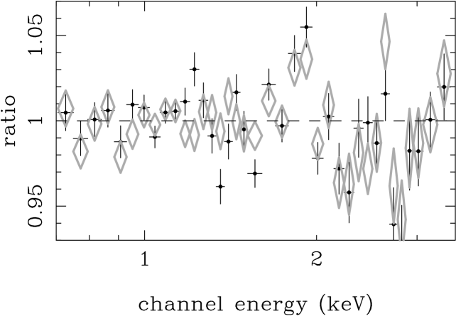
Figure 1: The data-to-model ratios of the deprojected spectra of the EMOS within $R$=2-8^′ fitted with the single temperature MEKAL model (black crosses) and version 1.1 of the APEC model (gray diamonds).

Table 1: Results of spectrum fitting of the deprojected spectra with the single temperature and the two temperature MEKAL model. For the outermost region, projected spectra are used. The regions with the enhanced X-ray emission associated with the radio structures are excluded throughout this paper.

$R$	kT1	kT2	$N_{\rm{H}}$	O	Si	S	Ar	Ca	Fe	$\chi^{2}/\mu^{a}$
(arcmin)	(keV)	(keV)	($10^{20}\rm{cm^{-2}}$)	(solar)	(solar)	(solar)	(solar)	(solar)	(solar)
The EMOS spectra fitted with a 1T MEKAL model
0.00- 0.35	1.13		4.1	0.02	0.37	0.37	1.01	1.25	0.20	435/177
0.35- 1.00	1.47		4.3	0.00	0.83	0.83	0.69	1.84	0.79	563/177
1.00- 2.00	1.56${}^{+0.03}_{-0.03}$		3.2${}^{+1.1}_{-1.1}$	0.42${}^{+0.14}_{-0.14}$	1.29${}^{+0.15}_{-0.14}$	1.09${}^{+0.17}_{-0.15}$	0.96${}^{+0.37}_{-0.36}$	2.66${}^{+0.88}_{-0.85}$	1.05${}^{+0.08}_{-0.07}$	177/175
2.00- 4.00	2.05${}^{+0.04}_{-0.04}$		1.3${}^{+0.6}_{-0.6}$	0.44${}^{+0.09}_{-0.09}$	1.24${}^{+0.10}_{-0.10}$	1.12${}^{+0.11}_{-0.10}$	0.71${}^{+0.20}_{-0.20}$	1.33${}^{+0.39}_{-0.39}$	1.07${}^{+0.06}_{-0.06}$	172/175
4.00- 8.00	2.30${}^{+0.04}_{-0.04}$		1.4${}^{+0.4}_{-0.4}$	0.45${}^{+0.07}_{-0.07}$	0.92${}^{+0.07}_{-0.07}$	0.71${}^{+0.08}_{-0.07}$	0.42${}^{+0.14}_{-0.16}$	1.01${}^{+0.28}_{-0.27}$	0.79${}^{+0.04}_{-0.04}$	199/175
8.00-11.30	2.51${}^{+0.08}_{-0.08}$		1.9${}^{+0.7}_{-0.7}$	0.37${}^{+0.12}_{-0.11}$	0.64${}^{+0.11}_{-0.10}$	0.35${}^{+0.12}_{-0.11}$	0.37${}^{+0.23}_{-0.24}$	0.72${}^{+0.42}_{-0.43}$	0.62${}^{+0.06}_{-0.06}$	243/175
11.30-13.50	2.72${}^{+0.06}_{-0.05}$		0.6${}^{+0.4}_{-0.4}$	0.32${}^{+0.07}_{-0.07}$	0.61${}^{+0.07}_{-0.06}$	0.20${}^{+0.07}_{-0.07}$	0.14${}^{+0.15}_{-0.14}$	0.49${}^{+0.24}_{-0.27}$	0.51${}^{+0.03}_{-0.03}$	275/175
The EMOS spectra fitted with a 2T MEKAL model
0.00- 0.35	1.56${}^{+0.19}_{-0.16}$	0.75${}^{+0.02}_{-0.02}$	2.3${}^{+1.5}_{-1.5}$	0.24${}^{+0.30}_{-0.23}$	1.04${}^{+0.62}_{-0.38}$	1.07${}^{+0.63}_{-0.43}$	0.62${}^{+1.07}_{-0.62}$	2.03${}^{+2.46}_{-2.03}$	0.85${}^{+0.39}_{-0.24}$	138/176
0.35- 1.00	1.73${}^{+0.04}_{-0.04}$	0.91${}^{+0.03}_{-0.03}$	2.1${}^{+0.8}_{-0.4}$	0.65${}^{+0.13}_{-0.12}$	1.70${}^{+0.17}_{-0.16}$	1.53${}^{+0.17}_{-0.16}$	0.99${}^{+0.28}_{-0.28}$	1.38${}^{+0.58}_{-0.57}$	1.54${}^{+0.12}_{-0.11}$	227/176
1.00- 2.00	1.68${}^{+0.06}_{-0.06}$	0.97${}^{+0.15}_{-0.15}$	2.6${}^{+1.1}_{-1.2}$	0.55${}^{+0.19}_{-0.16}$	1.56${}^{+0.26}_{-0.19}$	1.25${}^{+0.23}_{-0.18}$	0.96${}^{+0.41}_{-0.39}$	2.38${}^{+0.92}_{-0.87}$	1.28${}^{+0.09}_{-0.12}$	162/176
The EPN spectra fitted with a 1T MEKAL model
0.00- 0.35	0.74		9.0	0.19	0.32	0.71	3.15	0.40	0.08	255/132
0.35- 1.00	1.44		4.6	0.28	0.86	0.86	0.79	2.06	0.81	296/132
1.00- 2.00	1.56${}^{+0.05}_{-0.04}$		3.5${}^{+1.1}_{-0.5}$	0.45${}^{+0.15}_{-0.14}$	1.09${}^{+0.17}_{-0.16}$	0.99${}^{+0.22}_{-0.20}$	1.30${}^{+0.56}_{-0.54}$	1.70${}^{+1.28}_{-1.25}$	0.98${}^{+0.09}_{-0.08}$	112/125
2.00- 4.00	1.98${}^{+0.06}_{-0.06}$		1.5${}^{+0.7}_{-0.7}$	0.40${}^{+0.11}_{-0.10}$	1.05${}^{+0.14}_{-0.13}$	0.95${}^{+0.16}_{-0.15}$	0.81${}^{+0.35}_{-0.35}$	1.63${}^{+0.69}_{-0.68}$	0.96${}^{+0.08}_{-0.07}$	125/125
4.00- 8.00	2.28${}^{+0.06}_{-0.06}$		1.4${}^{+0.5}_{-0.6}$	0.28${}^{+0.09}_{-0.08}$	0.71${}^{+0.10}_{-0.10}$	0.53${}^{+0.13}_{-0.12}$	0.21${}^{+0.27}_{-0.21}$	1.01${}^{+0.50}_{-0.50}$	0.69${}^{+0.05}_{-0.05}$	93/125
8.00-11.30	2.48${}^{+0.10}_{-0.11}$		1.7${}^{+0.8}_{-0.9}$	0.29${}^{+0.16}_{-0.14}$	0.58${}^{+0.19}_{-0.17}$	0.28${}^{+0.21}_{-0.23}$	0.41${}^{+0.46}_{-0.41}$	0.95${}^{+0.81}_{-0.84}$	0.53${}^{+0.09}_{-0.07}$	85/125
11.30-16.0	2.54${}^{+0.07}_{-0.07}$		0.5${}^{+0.5}_{-0.4}$	0.26${}^{+0.07}_{-0.07}$	0.37${}^{+0.09}_{-0.08}$	0.33${}^{+0.12}_{-0.11}$	0.20${}^{+0.24}_{-0.20}$	0.38${}^{+0.39}_{-0.38}$	0.41${}^{+0.04}_{-0.04}$	190/131
The EPN spectra fitted with a 2T MEKAL model
0.00- 0.35	1.73${}^{+0.16}_{-0.18}$	0.73${}^{+0.02}_{-0.02}$	0.0${}^{+1.4}_{0.0}$	0.48${}^{+0.39}_{-0.27}$	1.23${}^{+0.57}_{-0.49}$	1.02${}^{+0.74}_{-0.61}$	1.27${}^{+1.77}_{-1.27}$	1.26${}^{+3.31}_{-1.26}$	1.08${}^{+0.32}_{-0.32}$	133/123
0.35- 1.00	1.73${}^{+0.05}_{-0.05}$	0.87${}^{+0.03}_{-0.03}$	0.9${}^{+1.0}_{-0.9}$	0.58${}^{+0.14}_{-0.13}$	1.47${}^{+0.26}_{-0.23}$	1.56${}^{+0.29}_{-0.25}$	0.96${}^{+0.48}_{-0.47}$	1.65${}^{+0.96}_{-0.93}$	1.55${}^{+0.18}_{-0.17}$	152/123
1.00- 2.00	1.77${}^{+0.09}_{-0.08}$	1.00 (fix)	0.8${}^{+1.4}_{-0.6}$	0.69${}^{+0.23}_{-0.20}$	1.73${}^{+0.41}_{-0.35}$	1.47${}^{+0.42}_{-0.36}$	1.60${}^{+0.78}_{-0.71}$	1.38${}^{+1.52}_{-1.38}$	1.49${}^{+0.26}_{-0.23}$	90/123

^a Degrees of freedom

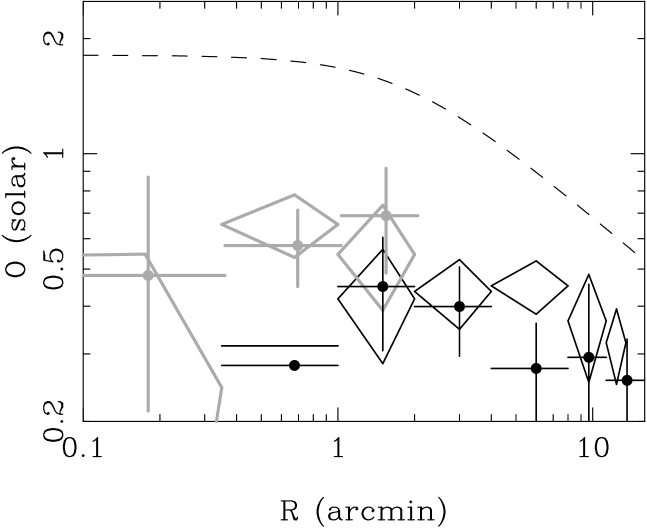
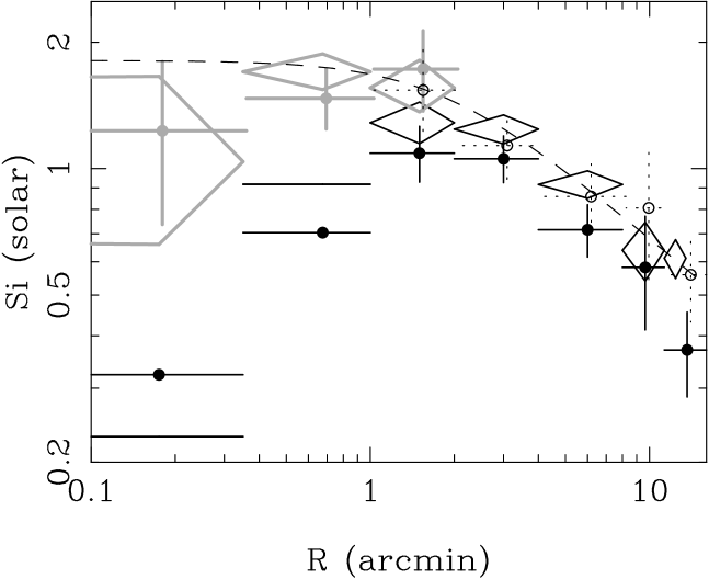
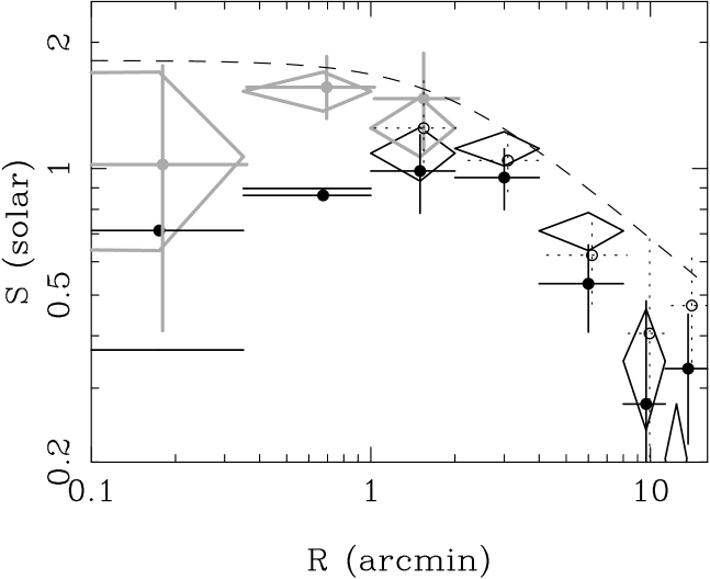
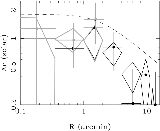
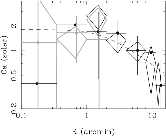
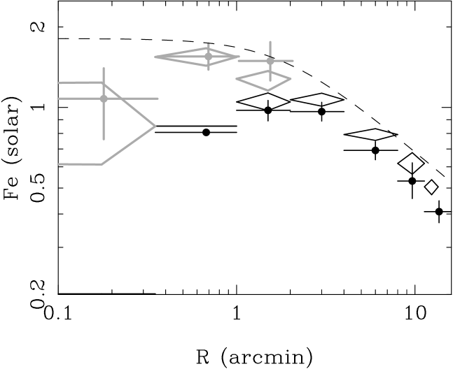
Figure 2: Abundance profiles of O, Si, S, Ar, Ca and Fe using the single temperature (black) and the two temperature (gray) MEKAL model from the deprojected data of the EMOS (diamonds) and the EPN (closed circles). The open circles are the Si and S abundances derived from the EPN spectra above 1.7 keV, when O, Ne, Mg, Fe and Ni abundances are fixed to be the best fit values derived from the EMOS data of the whole energy band. The dashed lines correspond to the best fit relation of the deprojected Si profile of the EMOS.

The results are summarized in Table 1 and Figures 1–4. Representative spectra fitted with the MEKAL model are shown in Figure 2 and 7 of Paper I and Figure 1. There remain small discrepancies between the data and the best fit model. A residual structure exists at 0.8–1 keV of the deprojected spectra of the EPN of $R>$2^′, when fitted with the single temperature MEKAL model, while the EMOS data have no such residual (Figure 2 of Paper I). Here, $R$ is the 3-dimensional radius. This problem will be discussed in the next paragraph. The Fe-L/Mg-K structure around 1.3 keV is not fitted well (Figure 1). Therefore, we do not show Mg abundances here and will discuss this in more detail below (Sec. 4 and 5.5-5.6). We also do not show Ne and Ni abundances, because their line strengths are much smaller than those of the Fe-L features at the same wavelength and a small uncertainty in the Fe-L complex gives large uncertainties in abundances of these elements (Masai 1987; Matsushita et al. 1997; 2000). There are also small discrepancies in the continuum level around K$\alpha$ lines of Si, S and Ar, which will be discussed in Sec. 5.

The derived abundances are mostly consistent between the EPN and the EMOS, although the EPN abundances of O, Si, S and Fe are systematically smaller than the EMOS results by 10–30%, when fitted with a single temperature MEKAL model. As will be shown in Sec. 5, the strengths of K$\alpha$ lines of H-like O, Si, S and He-like (+ Li like) Fe observed by the EPN and EMOS agree within several percent when considering the difference in the normalization between the two detectors. Therefore, these abundance discrepancies should be caused by the discrepancy at 0.8–1 keV, which may reflect uncertainties in an instrumental low energy tail of the strong Fe-L lines observed in EPN spectra, as discussed in Paper I. In addition, the EPN is characterized by a dependence of the energy resolution on the position on the detector. As a result, the observed Fe abundance of the EPN may be artificially decreased by these problems and the change of the continuum level also affects the O abundance. Those of Si and S also couple with abundances of other elements such as O and Fe due to the effect of free-bound emission and the increment of the strength of the Fe-L emission around the K$\alpha$ line of He-like Si. When we fix the O, Ne, Mg, Fe and Ni abundances to the best fit values derived from the EMOS spectra of the whole energy band and fitted the EPN spectra above 1.7 keV, we recover consistent Si and S abundances between the two detectors (Figure 2).

The derived abundances of Si, S, Ar, Ca, and Fe from deprojected spectra using the single temperature MEKAL model fit show strong negative gradients at $R>1^{\prime}$, and drop sharply within this radius (Table 1, Figure 2) as already seen in the projected spectra (Böhringer et al. 2001; Finoguenov et al. 2001; Gastaldello & Molendi 2002). But now the absolute values are slightly larger than those from projected spectra. In contrast, the O abundance is nearly constant at $R>1^{\prime}$.

The two temperature MEKAL fit on the deprojected spectra gives significantly larger abundances than the single temperature MEKAL fit (Figure 2-4, Table 1) and the central abundance drops seen in the single MEKAL fit become very week in the results of the two temperature MEKAL fit, although contributions of the cooler component are small as shown in Paper I. For example, at $R$=0.5-1’, 10 percent of the cooler component in units of emission measure changes the Fe abundances by a factor of 2. The reason for this is the change of the temperature of the hot component, when the cold component is added. For a fixed Fe line feature this leads to a higher abundance required in the fit. In addition, abundances of O, Si and S also increase by a factor of 2. The increment of the O abundance is due to the change of the temperature structure. The Si and S abundances increase due to an increment of the free-bound emission and the strength of Fe-L lines around the He-like Si line. Therefore, considering the remaining 1 keV temperature component associated with the radio structures within 2^′, abundances become nearly constant within 2^′.

We have also tried a three temperature MEKAL model for spectra within 2^′. Although the derived $\chi^{2}$ values have slightly improved, the derived abundances and their errors have nearly the same values as those from the two temperature MEKAL model fit.

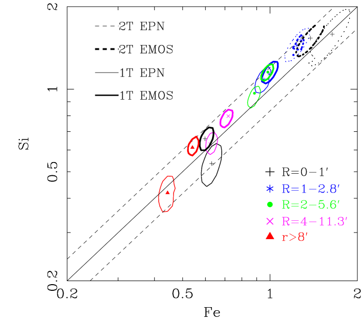
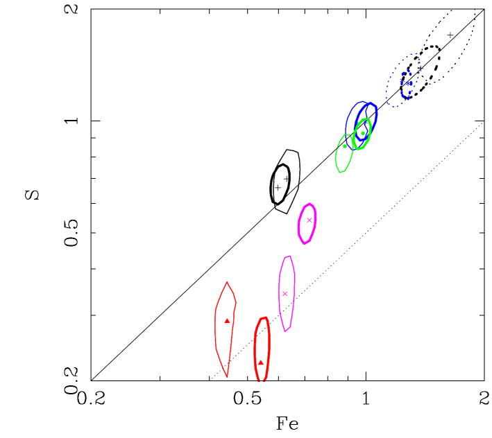
Figure 3: Confidence contours (90%) for the Si, S vs. Fe abundance of the deprojected data of the EMOS (thick lines) and the EPN (thin lines) fitted with the single temperature MEKAL model (solid lines) and the two temperature MEKAL model (dotted lines). For the outermost region, the projected spectra are used. The solid lines indicate the condition of the solar-abundance ratio. The dashed lines represent the Si/Fe ratio to be 0.8 and 1.2 solar and the dotted line represents the S/Fe ratio to be 0.5 solar.

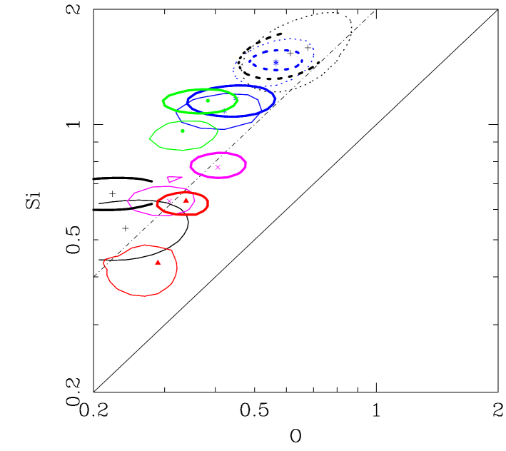
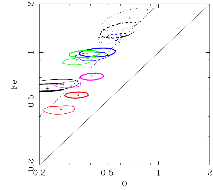
Figure 4: 90 % confidence contours for the Si, Fe vs. O. The meanings of the symbols are the same as in Fig. 3. The solid lines and dot-dashed lines represent the Si or Fe to O ratio to be 1 and 2 solar, respectively.

Figure 3 shows the confidence contours for the Si, S and Fe abundances, derived from the deprojected spectra. For the outermost region, the results from the projected spectra are plotted. The elliptical shape of the confidence contours indicates that abundance ratios are better determined than the abundances themselves. The differences in the Si/Fe and S/Fe ratios between the EMOS and EPN are considerably smaller than the abundance differences. Furthermore, the two temperature MEKAL model fit gives almost the same values of the Si/Fe and S/Fe ratio with the single temperature MEKAL model fit, although absolute values of Si, S, and Fe are largely changed. This means that the abundance ratios do not strongly depend on the temperature structure. As a result, the Si/Fe ratio is determined to be nearly constant at 1.1$\pm$ 0.1 solar, with no radial gradient. In contrast, we find that the S abundance has a steeper gradient than Fe abundance.

The abundances of Si and Fe are nearly independent to the O abundance (Figure 4). However, at the center, the two temperature MEKAL model gives the similar values of the O/Si and O/Fe ratio as the single temperature MEKAL model. The O/Si and O/Fe ratios are consistent between the two detectors, although the abundances of O, Si, and Fe between the EMOS and EPN differ by 10–30%. Both the Si/O and Fe/O ratios increase by a factor of 1.5 with radius. This result is in disagreement with the claim by Gastaldello & Molendi (2002), where they derived the constant Fe/O ratio. The background subtraction should not be a problem when determining O, Fe, and Si abundances, since even at the radius of 10^′, the background is only a few percent between 0.5 to 2 keV. In addition, the background was subtracted according to the detailed study by Katayama et al. (2002). A more severe problem should be the uncertainties in the response matrix, since the O abundance was inconsistent between the EPN and the EMOS by a factor of 2 using an old response matrix (Böhringer et al. 2001), although the discrepancy becomes smaller now as shown in this section. Using an old version of the response matrix and fitting the projected spectra in the same way in Gastaldello & Molendi (2002), we achieve the same results.

In summary, from the deprojected spectra using the MEKAL model, the abundances of Si, S, Ar, Ca, and Fe have steep gradients at $R>2^{\prime}$ and become nearly constant within the radius. The Si/Fe ratio is almost constant within the field of view, while the S/Fe ratio has a negative, and the O/Fe ratio has a positive gradient.

4 Spectral fits with the APEC model

A new plasma code, APEC (Smith et al. 2001), is now available in XSPEC_v11. Within the energy resolution of the CCD detectors, the dominant change from version 1.0 to the APEC code in the XSPEC version 11.0.1 is not in the Fe-L lines, but in the K$\alpha$ lines. Using version 1.0 of the APEC code, strengths of the K$\alpha$ lines of H-like ions, which are the most fundamental lines, decrease by $\sim$ 50 % at 2 keV, and their temperature dependences also change. The strength of the 6.7 keV Fe-K line decreases, by a factor of 2 at 1 keV and 1.3 at 4 keV. The changes of the K$\alpha$ lines of He-like ions of Si, S, Ar and Ca are smaller. As a result, any single temperature APEC model cannot fit the deprojected spectra of M 87, especially for the ratio of the Fe-L and the Fe-K as shown in Paper I, although a single temperature MEKAL model can fit each deprojected spectrum at $R>2^{\prime}$.

However, the strengths of K$\alpha$ lines of version 1.1 of the APEC code in version 11.1 of the XSPEC became more consistent with the MEKAL ones. Within the temperature range of the ICM of M 87, the largest differences except for the Fe-L structure are 20% changes in the strengths of the K$\alpha$ line of H-like O and the Fe line at 6.7 keV.

Using version 1.1 of the APEC code, we fitted the deprojected spectra of the EMOS. The results are summarized in Table 2 and Figure 5. In contrast to the worse $\chi^{2}$ values obtained from version 1.0 of the APEC code, version 1.1 gives similar $\chi^{2}$ values compared to those obtained by the MEKAL model. For the Fe-L/Mg-K structure around $\sim 1.4$ keV, the APEC (v1.1) model gives a better fit than the MEKAL model (Figure 1). The derived temperatures and hydrogen column densities are consistent with those from the MEKAL model. The contribution of the lower temperature component at $R$=1–2^′ has slightly decreased from 4% by the MEKAL code to 2% by the APEC code, although the contribution within 1^′ is consistent with each other. The few percent of the soft component using the MEKAL model at $R$=1–2^′ may be an artifact due to the uncertainties in the Fe-L complex.

Table 2: The results of the spectral fits of the deprojected spectra of the EMOS using the APEC (v1.1) code

$R$	kT1	kT2	$N_{\rm{H}}$	O	Mg	Si	S	Fe	$\chi^{2}/\mu^{a}$
(arcmin)	(keV)	(keV)	($10^{20}\rm{cm^{-2}}$)	(solar)	(solar)	(solar)	(solar)	(solar)
a 1T APEC model
0.00- 0.35	1.15		2.5	0.06	0.0	0.29	0.41	0.15	253/175
0.35- 1.00	1.48		2.4	0.97	1.17	1.80	1.79	1.37	583/175
1.00- 2.00	1.59${}^{+0.01}_{-0.03}$		2.8${}^{+1.2}_{-1.0}$	0.56${}^{+0.17}_{-0.08}$	0.87${}^{+0.17}_{-0.17}$	1.47${}^{+0.10}_{-0.08}$	1.28${}^{+0.15}_{-0.15}$	1.15${}^{+0.05}_{-0.05}$	126/175
2.00- 4.00	2.01${}^{+0.02}_{-0.01}$		2.1${}^{+0.3}_{-0.3}$	0.54${}^{+0.06}_{-0.09}$	0.67${}^{+0.12}_{-0.11}$	1.19${}^{+0.07}_{-0.06}$	1.09${}^{+0.08}_{-0.08}$	1.03${}^{+0.03}_{-0.02}$	181/175
4.00- 8.00	2.28${}^{+0.02}_{-0.03}$		2.0${}^{+0.2}_{-0.4}$	0.52${}^{+0.08}_{-0.05}$		0.87${}^{+0.06}_{-0.05}$	0.68${}^{+0.07}_{-0.06}$	0.78${}^{+0.02}_{-0.02}$	210/175
8.00-11.30	2.48${}^{+0.03}_{-0.03}$		2.2${}^{+0.7}_{-0.7}$	0.46${}^{+0.15}_{-0.11}$		0.65${}^{+0.08}_{-0.12}$	0.36${}^{+0.10}_{-0.14}$	0.64${}^{+0.06}_{-0.05}$	248/175
11.30-13.50	2.74${}^{+0.05}_{-0.07}$		0.8${}^{+0.5}_{-0.5}$	0.38${}^{+0.13}_{-0.08}$		0.62${}^{+0.07}_{-0.06}$	0.19${}^{+0.09}_{-0.08}$	0.53${}^{+0.03}_{-0.01}$	305/175
a 2T APEC model
0.00- 0.35	1.41${}^{+0.27}_{-0.43}$	0.78${}^{+0.03}_{-0.02}$	2.4${}^{+1.1}_{-1.5}$	0.26${}^{+0.29}_{-0.26}$	0.75${}^{+0.87}_{-0.31}$	1.14${}^{+0.96}_{-0.24}$	1.18${}^{+0.63}_{-0.42}$	0.96${}^{+0.10}_{-0.10}$	138/174
0.35- 1.00	1.78${}^{+0.06}_{-0.05}$	1.05${}^{+0.01}_{-0.02}$	2.0${}^{+0.8}_{-0.6}$	0.80${}^{+0.13}_{-0.14}$	1.10${}^{+0.14}_{-0.18}$	1.78${}^{+0.09}_{-0.16}$	1.61${}^{+0.11}_{-0.16}$	1.58${}^{+0.06}_{-0.14}$	190/174
1.00- 2.00	1.63${}^{+0.01}_{-0.01}$	1.00 (fix)	2.5${}^{+0.6}_{-1.2}$	0.64${}^{+0.23}_{-0.20}$	1.00${}^{+0.32}_{-0.27}$	1.61${}^{+0.27}_{-0.23}$	1.38${}^{+0.26}_{-0.22}$	1.26${}^{+0.17}_{-0.15}$	125/174

^a Degrees of freedom

Figure 5 compares the abundances derived from the APEC and the MEKAL model. The large abundance changes seen in APEC version 1.0 (Paper I) are not derived using the new APEC code, version 1.1. For Si, S, and Fe, we find consistent results within several percent. The O abundances from the APEC code are systematically larger than those from the MEKAL code by 20%, which is close to the difference of the line strength of the K$\alpha$ line of H-like O between the MEKAL and APEC model.

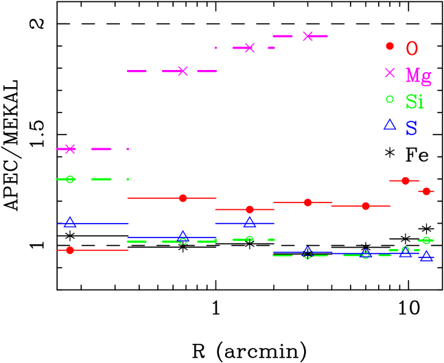
Figure 5: The ratios of the best fit abundances derived from the APEC model and MEKAL model. The two temperature model is used at $R<2^{\prime}$ and the single temperature model is used at $R>2^{\prime}$.

In contrast, the derived Mg abundances differ by a factor of 2 between the two codes. Since the APEC model can fit the Mg-K/Fe-L structure at $\sim$1.4 keV quite well, the APEC code may be better to derive a Mg abundance. There is another problem due to the strong instrumental line of the EMOS, which is located at a similar energy to the Mg line. At $r$=8–13.5^′, the strength of the instrumental line is a factor of 10 larger than the Mg line of the ICM, and the uncertainty affects the spectrum at $R$=4–8^′ through the deprojection. Here, $r$ is the projected radius from the center. Therefore, the Mg abundances are shown only within 4^′. The derived Mg abundance is $\sim 1$ solar at $R<2^{\prime}$ and shows a radial gradient outside this radius (Table 2).

The observed values of the Ne abundance derived from the APEC model are also a factor of 1.3 larger than those derived from the MEKAL model. For the Ni abundance, the APEC code gives 60% of the values from the MEKAL code at $R>2^{\prime}$, but within $R<2^{\prime}$, both codes give similar values. In contrast to the Mg lines, the Ni-L lines and the Ne-K lines cannot be distinguished in the spectra of M 87. Therefore, we do not present Ni and Ne abundances in this paper.

In summary, the new APEC code provides a better fit to the Fe-L structure, and the derived abundances of O, Si, and Fe are mostly consistent with those obtained from the MEKAL code. The Mg abundances are derived to be $\sim$ 1 solar at $R<2^{\prime}$, since the Fe-L/Mg-K structure is well fitted with the APEC code.

5 Abundance determination using line ratios

In this section, we try to obtain abundance ratios of elements directly from ratios of emission lines. When calculating the deprojected spectra, we make an assumption that spectra beyond the field of view are the same as the outermost spectrum, which is not valid since the temperature starts to decrease beyond the field of view of the detector (Shibata et al. 2001). Therefore, especially in the outer regions, there may be a bias due to this assumption, since emission lines have a stronger dependence on temperature than the continuum. In addition, abundances from deprojected spectra have a larger uncertainty due to poorer statistics than those derived from projected data. In order to derive abundances more accurately, we need projected spectra.

However, the projected spectra consist of multi-temperature components. As a result, some line ratios, such as the ratio of K$\alpha$ lines of He- and H-like S, of the projected spectra cannot be fitted with a single temperature MEKAL model (Figure 6). We must be careful in using a multi-temperature model, e.g. a two temperature model, since emission lines and a continuum spectrum are different functions of temperature. In addition, the continuum spectra between S, Ar and Ca lines show small discrepancies between the data and the single temperature model. These small discrepancies sometimes give larger uncertainties in the strengths of faint lines such as K$\alpha$ lines of He-like Ar and Ca. For example, when fitting with a single temperature MEKAL model with the projected spectrum at 2–4^′, temperature and Ar abundance are determined as 2.2 keV and 0.7 solar, respectively. However, when we restrict the energy range within 2.8–5.0 keV and fix the abundances of O, Ne, Mg, Si, S and Fe to the best fit values obtained from the whole energy band fit, the temperature becomes 2.4 keV and Ar abundance is determined as 1.1 solar. Here, the Ar abundance is changed by 60%, although the best fit temperatures differ by only 10%. This small discrepancy between the S and Ar lines is also seen in the deprojected spectra, although their errors are larger.

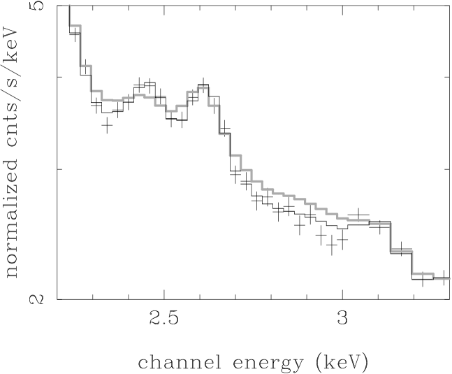
Figure 6: The projected EMOS spectrum of $r$=8.0-13.5^′ (crosses) fitted with a single MEKAL model (gray) and bremstrallung and gaussians (black).

Table 3: Ratios of K$\alpha$ lines and abundance ratios (errors correspond to 68%). Within 2^′, the effect of the lower temperature component is considered.

r	H-O/H-Si	O/Si (solar)	(H-S+He-S)/H-Si	S/Si (solar)	He-Ar/H-Si	Ar/Si (solar)	He-Ca/H-S	Ca/S (solar)
Annular spectra of the EMOS
0.0- 0.5	$2.26\pm 0.29$	$0.43\pm 0.06$	$1.08\pm 0.06$	$1.14\pm 0.06$	$0.16\pm 0.03$	—	$0.20\pm 0.04$	—
0.5- 1.0	$2.16\pm 0.15$	$0.48\pm 0.03$	$1.02\pm 0.04$	$1.05\pm 0.05$	$0.14\pm 0.02$	$0.79\pm 0.11$	$0.23\pm 0.03$	$1.29\pm 0.16$
1.0- 2.0	$1.90\pm 0.11$	$0.45\pm 0.03$	$0.94\pm 0.03$	$0.96\pm 0.03$	$0.18\pm 0.03$	$0.87\pm 0.12$	$0.28\pm 0.03$	$1.53\pm 0.15$
2.0- 4.0	$1.84\pm 0.13$	$0.46\pm 0.03$	$0.93\pm 0.03$	$0.97\pm 0.03$	$0.17\pm 0.01$	$0.78\pm 0.06$	$0.23\pm 0.02$	$1.16\pm 0.10$
4.0- 8.0	$2.38\pm 0.10$	$0.59\pm 0.02$	$0.82\pm 0.03$	$0.87\pm 0.03$	$0.14\pm 0.02$	$0.67\pm 0.09$	$0.24\pm 0.02$	$1.18\pm 0.11$
8.0-13.5	$2.45\pm 0.20$	$0.61\pm 0.05$	$0.62\pm 0.05$	$0.67\pm 0.05$	$0.14\pm 0.03$	$0.71\pm 0.16$	$0.32\pm 0.06$	$1.56\pm 0.29$
Deprojected spectra of the EMOS
0.0- 0.5	$2.08\pm 0.42$	$0.35\pm 0.07$	$1.09\pm 0.17$	$1.16\pm 0.18$	$0.18\pm 0.06$	—	$0.18\pm 0.08$	—
0.5- 2.0	$2.06\pm 0.23$	$0.45\pm 0.05$	$0.96\pm 0.04$	$1.00\pm 0.04$	$0.16\pm 0.02$	$0.93\pm 0.11$	$0.29\pm 0.04$	$1.60\pm 0.21$
2.0- 5.6	$1.77\pm 0.12$	$0.44\pm 0.03$	$0.90\pm 0.04$	$0.93\pm 0.04$	$0.18\pm 0.02$	$0.85\pm 0.10$	$0.24\pm 0.03$	$1.24\pm 0.16$
5.6-11.3	$2.74\pm 0.31$	$0.68\pm 0.08$	$0.75\pm 0.07$	$0.80\pm 0.08$	$0.14\pm 0.03$	$0.67\pm 0.15$	$0.25\pm 0.05$	$1.26\pm 0.26$
Annular spectra of the EPN
0.0- 0.5	$2.00\pm 0.33$	$0.38\pm 0.06$	$1.11\pm 0.11$	$1.17\pm 0.11$	$0.30\pm 0.05$	—	$0.24\pm 0.09$	—
0.5- 1.0	$1.87\pm 0.20$	$0.41\pm 0.04$	$1.04\pm 0.06$	$1.07\pm 0.06$	$0.15\pm 0.03$	$0.81\pm 0.13$	$0.24\pm 0.06$	$1.36\pm 0.31$
1.0- 2.0	$1.90\pm 0.18$	$0.44\pm 0.07$	$0.92\pm 0.05$	$0.94\pm 0.05$	$0.18\pm 0.02$	$0.88\pm 0.10$	$0.28\pm 0.04$	$1.50\pm 0.22$
2.0- 4.0	$1.87\pm 0.23$	$0.47\pm 0.06$	$0.93\pm 0.05$	$0.97\pm 0.05$	$0.17\pm 0.02$	$0.81\pm 0.11$	$0.35\pm 0.05$	$1.78\pm 0.25$
4.0- 8.0	$2.09\pm 0.26$	$0.52\pm 0.06$	$0.76\pm 0.05$	$0.82\pm 0.05$	$0.08\pm 0.02$	$0.41\pm 0.09$	$0.34\pm 0.09$	$1.69\pm 0.44$
8.0-13.5	$2.70\pm 0.43$	$0.67\pm 0.11$	$0.67\pm 0.08$	$0.73\pm 0.09$	$0.20\pm 0.05$	$1.02\pm 0.23$	$0.44\pm 0.08$	$2.14\pm 0.39$

Therefore, in this section, we determine strengths of emission lines, and then determine abundance ratios, considering the temperature dependence of line ratios. We have fitted the projected and deprojected spectra within an energy band around a given line with thermal bremsstrahlung and gaussians. Obtaining strengths of K$\alpha$ lines of He-like S and Ar, contributions of K$\beta$ lines of H-like Si and S were subtracted using the strengths of K$\alpha$ lines. Here, we used the K$\beta$ to K$\alpha$ ratio of the MEKAL code. Strengths of H-like K$\alpha$ lines of O were obtained from spectra within the energy range of 0.55–1 keV fitted with a gaussian and two APEC models with zero O abundance. Those of Si were also obtained from fitting with gaussians and the two temperature APEC model with zero Si abundance, using the 1.1–2.2 keV energy band. We selected line ratios whose temperature dependence is small, for accurate measurements of abundance ratios. The results are summarized in Table 3.

5.1 O vs. Si

The abundance ratio of O/Si is better obtained from the ratio of the line strengths of K$\alpha$ lines of H-like ions. Although the O and Si abundances obtained from the EMOS and the EPN using the same single temperature model have small discrepancies of 20$\sim$ 30%, the line ratios of the two detectors agree well with each other (Figure 7).

The observed radial profile of the line ratio has a minimum at $\sim$2^′ (Figure 7). Figure 7 also shows the line ratios plotted against the best fit MEKAL temperatures from the whole energy band. When the abundance ratio of O/Si is constant, the line ratio is almost constant above 1.7 keV and it starts to increase sharply below the lowest temperature. Comparing the observed minimum value of $\sim$ 2 with the minimum value of $\sim 4$ corresponding to the solar abundance ratio, no temperature distribution can reproduce an O/Si ratio larger than 0.5 solar at the radius of $\sim$2^′.

Considering the temperature structure derived in Paper I, we can better constrain the O/Si ratio. The independence of the line ratio from the temperature above 1.7 keV means that the abundance ratio can be directly obtained dividing the line ratio by that of the solar abundance ratio when there is no temperature component below 1.7 keV. Thus, beyond $2^{\prime}$, the gradient of the line ratio reflects a change of the O/Si ratio, since outside 2^′, there is no temperature component below 1.7 keV (Paper I). From the line ratio at $r$= 2–4^′, the O/Si is derived to be 0.46 solar, and beyond $r>8^{\prime}$, it increases to 0.6–0.7 solar (Figure 7).

Within 2^′, the presence of the additional $\sim$ 1 keV temperature component must be considered. The derived O/Si ratio assuming that the temperature is larger than 1.7 keV should be the maximum value of the O/Si ratio which is $\sim$ 0.5 solar within 2^′ (triangles in the bottom panel of Figure 7). We also derive the O/Si ratio from the line ratio considering the fraction of the low temperature component, which is derived from the spectral fit using the best fit two temperature APEC model. Then, the O/Si ratio is derived to be 0.45 solar at 1–2^′ and 0.4 solar within 0.5^′. Since the line ratio is a steep function when the temperature is around 1 keV, we have also checked a case when the lower temperatures is 0.6 keV, which is 0.2 keV smaller than the central temperature. For the innermost region, the derived O/Si ratio with the temperature of 0.6 keV is consistent within 10 percent, since the temperature of the softer component becomes lower, the fraction of the component also becomes lower which is derived from the spectral fitting from Fe-L.

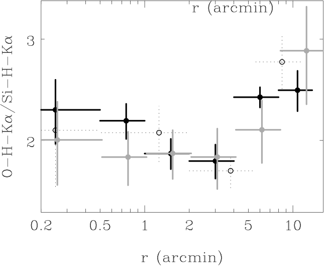
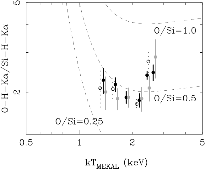
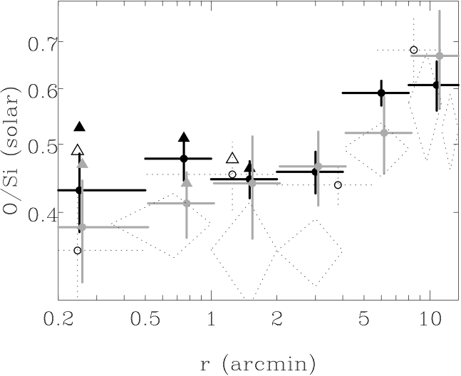
Figure 7: The line ratios of K$\alpha$ lines of H-like O and Si of the EMOS (black) and the EPN (gray), plotted against the radius (upper panel) and the best fit temperature fitted with the single MEKAL model (middle panel). Solid and dotted data correspond to projected and deprojected data, respectively. Dashed lines in the middle panel correspond to constant abundance ratios in unit of the solar ratio. The derived abundance ratios are plotted in the bottom panel. Within 2 arcmin, contributions of the lower temperature component are considered. Triangles are the best fit values of the abundance ratio, assuming the temperature is larger than 1.7 keV. The diamonds correspond to the abundance ratios derived from the deprojected EMOS spectra using the MEKAL model fit. Errors represent the 68% confidence level.

For comparison, we also plotted the O/Si ratio derived from the deprojected spectra through the spectral fits and the line ratio. Although the O/Si ratios derived from the line ratios are systematically larger by $\sim$ 20% than those derived from spectral fit with the MEKAL model, the gradient of the O/Si ratio is consistent between the two, and the O/Si ratio changes by a factor of 1.4 from the center to 10^′.

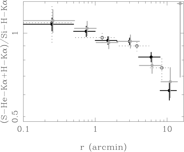
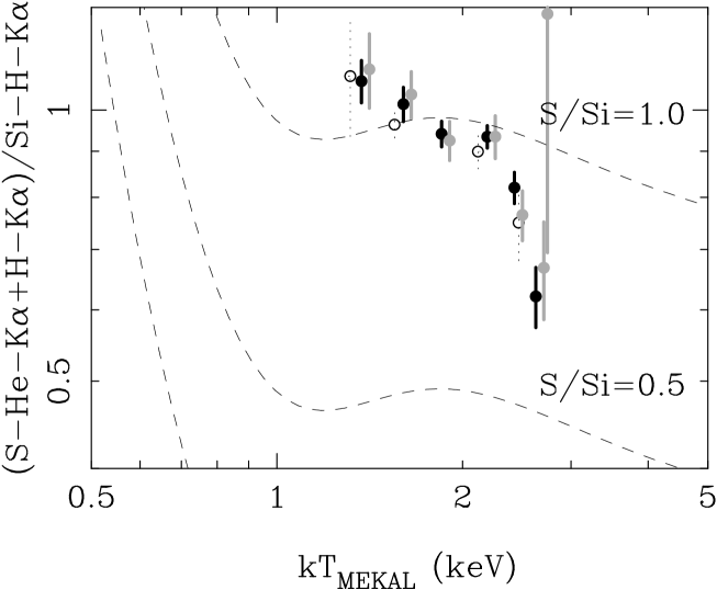
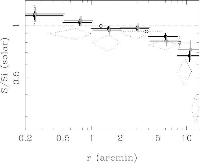
Figure 8: The line ratios of K$\alpha$ lines of the sum of He-like and H-like S to H-like Si of the EMOS (black) and the EPN (gray), plotted against radius (top panel) and temperature (middle panel), and the radial profile of the S/Si ratio (bottom panel). The meaning of the symbols are the same as in Figure 7. Errors represent the 68% confidence level.

5.2 S vs. Si

Although the ratios of K$\alpha$ lines of He-like or H-like S to that of H-like Si are both steep functions of temperature, the ratio of the sum of the two K$\alpha$ lines of S to the H-like Si line is nearly constant within 10% between 0.9 to 5 keV when the S/Si ratio is constant (Figure 8). The important point is that we can derive the abundance ratio almost independently from the temperature structure of the ICM. Considering that there is no temperature component below 1 keV, as in the case of the O/Si ratio, even for the projected data, the S/Si ratio can be directly calculated from the line ratio. As in the previous subsection, the effect of the lower temperature component is estimated to be less than a few percent.

The observed profile of the line ratio shows a negative gradient and at $r$=10^′, it is about half of the central value. This gradient reflects the change of the S/Si ratio, because of the small dependence on temperature. Converted to the abundance ratio, the S/Si ratio is 1.0 solar within 2^′, and drops to 0.67 solar at $\sim$ 10^′ (Figure 8). These results are systematically larger than those derived from the spectral fits. Especially, at $r>8^{\prime}$, the spectral fits on the projected spectra give the S/Si ratio to be 0.3–0.5 solar (Table 1, Figure 2), while the line ratio gives the value of 0.6–0.7 solar. For the projected data, the S abundance from the spectral fit should not be correct since the single temperature model cannot fit the two K$\alpha$ lines simultaneously as shown in Figure 6.

5.3 Ar vs. Si

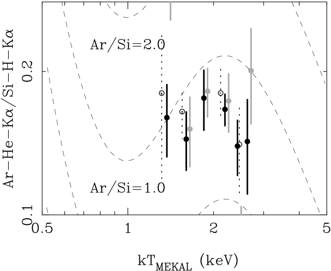
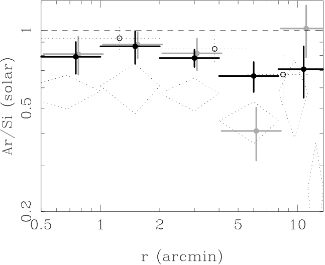
Figure 9: The line ratios of K$\alpha$ lines of He-like Ar to H-like Si of the EMOS (black) and the EPN (gray) (top panel) and the Ar/Si ratio (bottom panel). The meaning of the symbols are the same as in Figure 7. Errors represent the 68% confidence level.

Although the line ratio of the K$\alpha$ lines of He-like Ar to H-like Si is a steeper function of temperature than S/Si or O/Si ratio, within 1.7 to 2.8 keV, at a given ratio of Ar/Si, the change of the line ratio is less than 10 % (Figure 9). In Paper I, we found that at $R>0.5^{\prime}$, the ICM temperature at a given radius is dominated by a single temperature component whose temperature is larger than 1.7 keV. From Figure 7 in Paper I, the contributions from the 1 keV component to Ar and H-like Si lines are negligible. Therefore, as in case of the S to Si abundance ratio, we can obtain the abundance ratio of Ar/Si from the line ratio. The results indicate that the Ar/Si is 0.7–0.8 solar.

The derived Ar/Si ratios are systematically larger than the results of the spectral fit on the projected data (Finoguenov et al. 2002) by 30% within 3^′ and by a factor of 2 at $r>8^{\prime}$. This large discrepancy is caused by the failure to fit the continuum between the S and Ar lines illustrated in Figure 6.

5.4 Ca vs. S

The ratio of the K$\alpha$ line of the He-like Ca to that of the H-like S also show a small temperature dependency (Figure 10). Because these lines are dominated by a hotter temperature component even around the center, we can calculate the Ca/S ratio in the same way. The Ca/S ratio is $\sim$ 1.5 solar within the whole region.

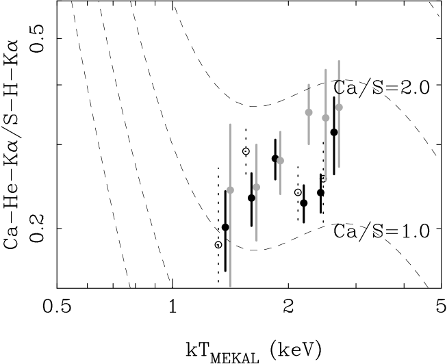
Figure 10: The line ratios of K$\alpha$ lines of He-like Ca to H-like S of the EMOS (black) and the EPN (gray). The meaning of the symbols are the same as in Figure 7. Errors represent the 68% confidence level.

5.5 Mg vs. O

The energy of the K$\alpha$ line of H-like Mg is slightly shifted from the peak of the Fe-L emission at $\sim$ 1.49 keV (Figure 11). Thus, the K$\alpha$ line can be distinguished within the energy resolution of the CCDs. The problem with the spectral fitting is the modeling of the Fe-L structure around the Mg line. Due to the problem of the strong instrumental line of the EMOS, we do not present the results on the Mg-K line for $r>8^{\prime}$.

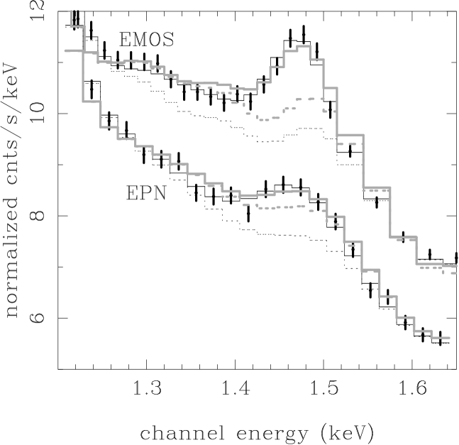
Figure 11: The projected spectra of $r$=2-4^′ at the energy band of Mg of the EMOS and the EPN fitted with the two temperature APEC model with zero Mg abundance (black dotted lines) and gaussians. Those using the MEKAL model are shown as gray lines.

The strengths of H-like and He-like K$\alpha$ lines of Mg were obtained from spectra within 1.1–1.6 keV, fitted with gaussians and a two temperature MEKAL or APEC model with zero Mg abundance. The results are summarized in Table 4.

Figure 12 shows the ratios of the K$\alpha$ line of the H-like Mg to that of H-like O. The strengths of the Mg line obtained using the APEC Fe-L model are $\sim$ 30% larger than those derived using the MEKAL model. Since the APEC fit to the Fe-L/Mg-K feature of 1.4 keV is better than the MEKAL model fit, the APEC code may be better to describe the Fe-L feature, although the discrepancy between the data and model of the MEKAL plus gaussians is only several percent.

Table 4: Line ratio of K$\alpha$ of H-like Mg, O, and Si and their abundance ratios, when the Fe-L is modeled with the APEC (errors correspond to 68%)

r	H-Mg/H-O	Mg/O (solar)	H-Mg/H-Si	Mg/Si (solar)
Annular spectra of the EMOS
0.0- 0.5	$0.23\pm 0.04$	$1.46\pm 0.23$	$0.53\pm 0.05$	$0.63\pm 0.07$
0.5- 1.0	$0.22\pm 0.02$	$1.33\pm 0.11$	$0.48\pm 0.03$	$0.64\pm 0.04$
1.0- 2.0	$0.21\pm 0.02$	$1.26\pm 0.14$	$0.40\pm 0.04$	$0.57\pm 0.06$
2.0- 4.0	$0.22\pm 0.02$	$1.30\pm 0.14$	$0.40\pm 0.03$	$0.59\pm 0.05$
4.0- 8.0	$0.19\pm 0.02$	$1.16\pm 0.10$	$0.46\pm 0.04$	$0.69\pm 0.06$
Deprojected spectra of the EMOS
0.0- 0.5	$0.27\pm 0.07$	$1.73\pm 0.48$	$0.56\pm 0.13$	$0.61\pm 0.14$
0.5- 2.0	$0.20\pm 0.03$	$1.19\pm 0.17$	$0.41\pm 0.04$	$0.54\pm 0.05$
2.0- 4.0	$0.20\pm 0.05$	$1.21\pm 0.28$	$0.42\pm 0.08$	$0.66\pm 0.10$
Annular spectra of the EPN
0.0- 0.5	$0.31\pm 0.06$	$1.90\pm 0.36$	$0.61\pm 0.08$	$0.72\pm 0.10$
0.5- 1.0	$0.22\pm 0.04$	$1.31\pm 0.22$	$0.41\pm 0.06$	$0.54\pm 0.07$
1.0- 2.0	$0.19\pm 0.03$	$1.14\pm 0.20$	$0.36\pm 0.06$	$0.52\pm 0.08$
2.0- 4.0	$0.23\pm 0.05$	$1.41\pm 0.31$	$0.44\pm 0.08$	$0.65\pm 0.13$
4.0- 8.0	$0.24\pm 0.06$	$1.45\pm 0.38$	$0.50\pm 0.12$	$0.75\pm 0.18$
8.0-13.5	$0.15\pm 0.04$	$0.94\pm 0.26$	$0.41\pm 0.10$	$0.63\pm 0.15$

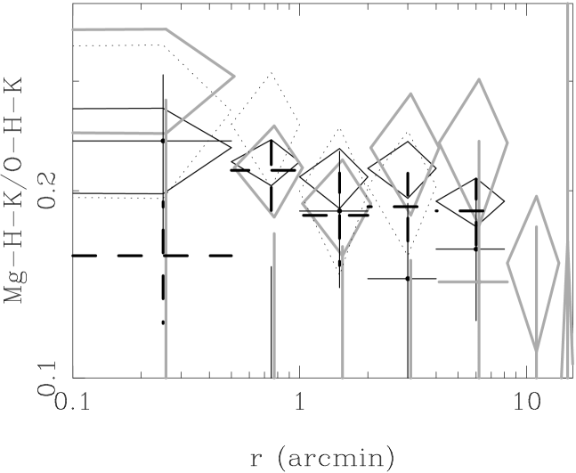
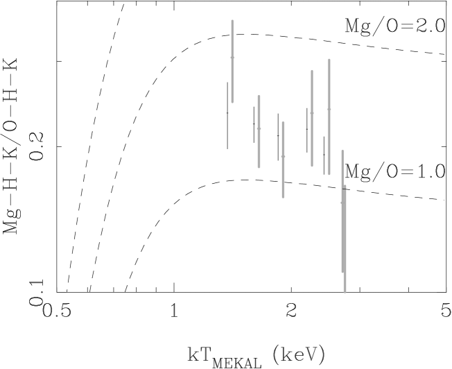
Figure 12: (Top panel) The ratio of strength of K$\alpha$ lines of H-like Mg and O of the projected spectra of the EMOS (black) and EPN (gray). The Fe-L is modeled with the APEC (diamonds) and the MEKAL (crosses) and bremsstrahlung and gaussians (bold dashed lines). The results of the deprojected spectra of the EMOS, where the Fe-L lines are modeled with the APEC are shown as dotted diamonds. (Bottom panel) The line ratios when the Fe-L lines are modeled with the APEC are plotted against the best fit temperature fitted with the single MEKAL model. Dashed lines correspond to constant abundance ratios. Errors represent the 68% confidence level.

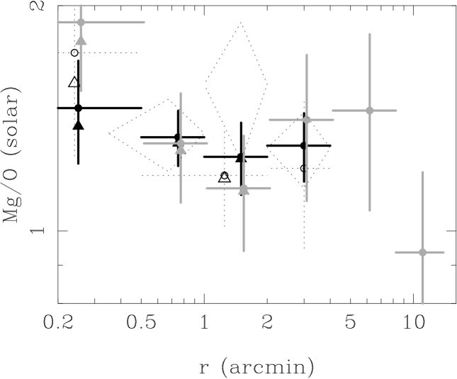
Figure 13: The Mg/O ratio derived from the line ratio, where the Fe-L lines are modeled with the APEC code. The meaning of the symbols are the same as in Figure 7. The dotted diamonds correspond to the abundance ratios of the EMOS derived from the APEC model fit to the deprojected spectra. Errors represent the 68% confidence level.

The projected EMOS spectra in the energy range of 1.35 to 1.6 keV are also fitted with a bremsstrahlung model plus two gaussians at 1.47 keV and 1.49 keV, since the K$\alpha$ line of H-like Mg at 1.47 keV and a Fe-L peak at 1.49 can be distinguished within the EMOS energy resolution (Figure 11). Freeing the strength of 1.49 keV peak of the Fe-L enable us to constrain the Mg line strength. The derived strengths of the Mg line are consistent with those derived using the APEC code for the modeling of the Fe-L. This result supports the Mg line strengths from the APEC code than those from the MEKAL code.

As in Sec. 5.1-5.4, we have plotted the line ratio from the APEC code against the best fit MEKAL temperature (Figure 12). The constant Mg/O ratio gives a constant line ratio within 10% above 1 keV. As in Sec. 5.1, we have estimated the effect of the temperature component below 1 keV, which is less than 10% for the innermost region. The derived Mg/O ratios are about 1.2–1.3 solar with no radial gradient at $r>0.5^{\prime}$, when we adopt the Fe-L modeling for the APEC (Figure 13). Within 0.5^′, a higher Mg/O ratio is allowed, since adding a temperature component blow 1 keV, the Mg/O ratio increases.

The O and Mg abundances obtained from the RGS spectrum through a spectral fit are 0.49$\pm 0.04$ solar and 0.9$\pm 0.2$ solar, respectively (Sakelliou et al 2002). This Mg/O ratio derived from the RGS is a factor of 1.5 larger than that at $r>0.5^{\prime}$ derived from the EMOS spectra using the APEC code for modeling the Fe-L. Since most of the photons detected by the RGS come from the very center, where a larger Mg/O ratio is also allowed by the EMOS data, the Mg/O ratio may increase at the center.

5.6 Mg vs. Si

The derived ratios of the K$\alpha$ lines of H-like Mg and Si are summarized in Table 4 and Figure 14. Here, only the result using the APEC code for the Fe-L modeling is shown. The temperature dependence of the line ratio is quite similar to that of the K$\alpha$ lines of O and Si, and the Mg/Si ratio was derived in the same way as in Sec. 5.1. Within 2^′, the contribution of the 1 keV component is taken into account. The derived Mg/Si ratio is $\sim 0.6$ solar, which agrees well with the ratio derived from the spectral fit using the APEC model in Sec 4.

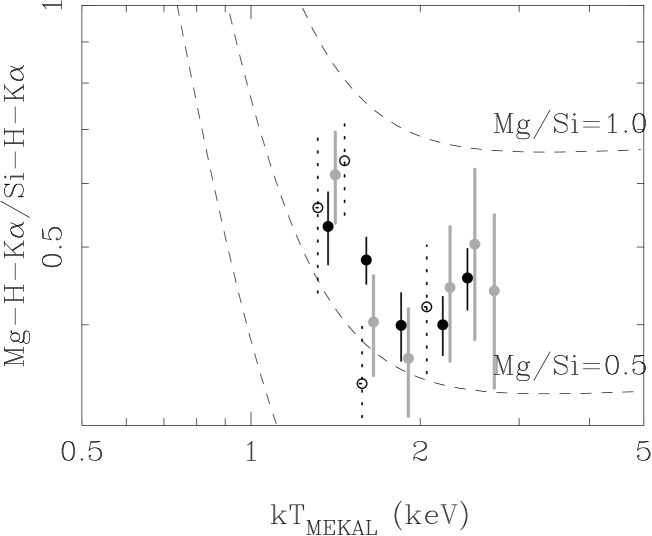
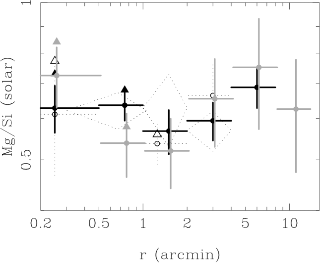
Figure 14: (Top panel) The ratio of strength of K$\alpha$ lines of H-like Mg and Si plotted against the best fit temperature fitted with the single MEKAL model. The Fe-L is modeled with the APEC. Dashed lines correspond to constant abundance ratios. The meanings of the symbols are the same as in Figure 7. (Bottom panel) The radial profile of the Mg/Si ratio derived from the line ratio. The dotted diamonds are the Mg/Si ratios derived from the spectral fitting using the APEC code. Errors represent the 68% confidence level.

5.7 Fe vs. Si

In contrast to the temperature dependences of the line ratios in the previous subsections, the ratio of the Fe-K line at 6.7 keV (which includes He and Li like ions) to the K$\alpha$ line of the H-like Si line strongly depends on temperature. For example, at 2 keV, a 10 % increment of temperature increases the Fe/Si ratio by 36 %. As a result, small uncertainties in the temperature structure give large uncertainties in the abundance ratios. Therefore, the Si/Fe ratio cannot obtained from the line ratio as in previous subsections. Since this ratio is quite important, we have calculated the Si/Fe line ratio of the projected data using the temperature structure obtained in Paper I and compared it with the observed profile (Figure 15). We used the relation of $kT=1.68(1+(R/1.6^{\prime})^{2})^{0.115}$ keV, since the hotter component dominates these lines even within 2^′. Assuming the Fe/Si ratio is approximated by $a+bR$, where a and b are free parameters, we fitted the profile of the line ratio. The radial profile of the line ratio is well fitted with the model ($\chi^{2}$=7.67 for 9 degrees of freedom) and the Fe/Si ratio is determined to be $\sim$ 0.9 solar within the whole field of view (Figure 15), although the abundance ratio changes by 20% when the whole temperature is shifted by 5%. Considering that the value of 0.9 solar is quite close to the ratio derived from the spectral fitting of the deprojected data, where the Fe abundance is determined by the Fe-L emission, the Fe/Si ratio should be $\sim$ 0.9 solar and its radial gradient is less than 10–20%.

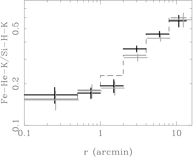
Figure 15: (upper panel) The radial profile of projected line ratios of the EMOS (black) and EPN (gray) between K$\alpha$ of H-like Si and He-like Fe. Errors correspond to 68% confidence level. The dashed line represents the best fit model using the temperature profile obtained in Paper I. (lower panel) 90 % confidence contour of the Fe/Si at $R$=14^′ vs. that at $R$=1^′ obtained from the ratio of the K$\alpha$ line of the He+Li-like Fe to H-like Si of the projected data, assuming Fe/Si=$a+bR$ and kT=$1.68(1+(R/1.6^{\prime})^{2})^{0.115}$ (keV). The cross is the correlation derived from the deprojected spectra, determined from the Fe-L emission.

6 Effect of resonance line scattering

Some resonant lines may become optically thick in the dense cores of clusters. Shigeyama (1998) calculated the effect on M 87 and several X-ray luminous elliptical galaxies, and found that it should be important at the center. Böhringer et al. (2001) suggested that the observed central abundance drop may be due to the effect. In the case of an X-ray luminous elliptical, NGC 4636, Xu et al. (2002) discovered direct evidence of resonant scattering using a line ratio between optically thick and thin lines.

The profile of optical depth for resonant lines of some prominent emission lines are calculated in Böhringer et al. (2001). Using the observed abundance profiles (Table 1), the temperature profile used in Sec. 5.7 and the density profile derived in Paper I, optical depths from the center for K$\alpha$ lines of H-like Si and O are calculated to be 1 and 0.4, respectively. Therefore, we must evaluate the effect of the scattering, although the central abundance drop is very small when fitted with the two temperature MEKAL model.

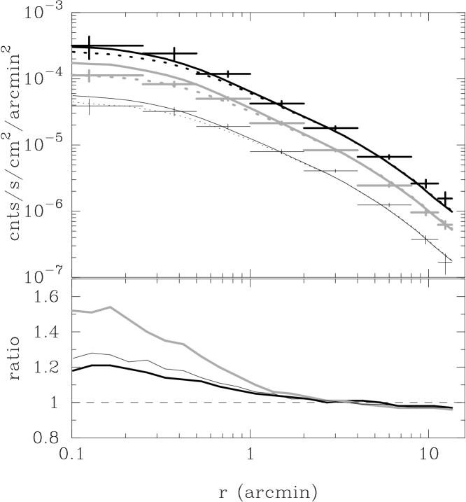
Figure 16: Radial profile of brightness of H-like ions of O (bold black lines), Si (gray lines), and S (thin black lines). Crosses are observed profiles and solid and dotted lines corresponds to the simulated profiles before and after resonant line scattering, respectively. The bottom panel shows the ratios of the profiles of before and after the scattering.

Ignoring turbulent motion, we have calculated the effect of resonant line scattering on the K$\alpha$ lines of H-like ions, using Monte-Carlo simulations.

The results are summarized in Figure 16. The scattered profiles of lines are consistent with those ignoring scattering beyond 1^′. Within this radius, the brightness of the lines decrease. The reduction rates at 0.5^′ are 10, 30, 15% for O, Si, and S, respectively. The effect is important only within 0.5^′ on the Si line, where the uncertainty in temperature structure also gives an uncertainty in abundance determination.

7 Discussion

7.1 Summary of abundances

The abundance profiles of O, Si, S, Ar, Ca and Fe are obtained from the deprojected spectra, based on the temperature study in Paper I. Although version 1.0 of the APEC code gives significantly different results (Paper I), version 1.1 of the APEC code gives consistent results with those of the MEKAL code for these elements. Within 2^′, considering the two temperature nature of the ICM, the abundance profiles from deprojected spectra become almost constant. Within this radius, the Si, S, Ar, Ca and Fe abundances are $\sim$ 1.5 solar, while the O abundance is a factor of 2 smaller. Using the APEC code, the Mg abundance is derived to be $\sim$ 1 solar at the center, since the APEC code gives a better fit on the Fe-L/Mg-K structure at 1.4 keV. Beyond 2^′, Si, S, Ar, Ca and Fe show strong negative gradients, while the abundance gradient of O is smaller. The Si/Fe ratio is 1.1 solar, with no gradient in the field of view.

The projected and deprojected profiles of abundance ratios are also obtained through line ratios. Since some line ratios among $\alpha$-elements are nearly constant within the temperature range of the ICM around M 87, the abundance ratios are obtained with better accuracy. From the temperature dependence of the line ratio, we can conclude that the low O/Si ratio cannot be explained by any temperature model, and the ratios of O/Si are 0.4–0.5 solar at the center and 0.6–0.7 solar at the outer region. The Mg/O ratio is determined to be 1.2–1.3 solar. The Ar and S abundances thus obtained are systematically larger than the spectral fit results due to small disagreements in the continuum fits around these lines. The S/Si is 1.1 solar at the center and 0.7 solar at outer regions. The Si/Fe ratio derived from the projected profile of the K$\alpha$ line ratio is consistent with that derived from the deprojected spectra through the spectral fit, where the Fe abundance is determined by the Fe-L structure.

The observed abundance pattern is similar to those obtained for A 496 (Tamura et al. 2001), and NGC 4636 (Xu et al. 2002). Therefore, this abundance pattern may be uniform around the central galaxies of groups or clusters.

7.2 Comparison of the abundance pattern with Galactic stars

Figures 17 and 18 show the observed abundance ratios of O, Mg, Si, Ca and Fe compared to those of the Galactic disk stars (Edvardsson et al. 1993). The average abundance ratios of low metallicity (i.e. [Fe/H]$<$-0.8) stars of the Galaxy by Clementini et al. (1999), which should reflect the average abundance pattern of SN II products of our Galaxy are also plotted. Other papers on Galactic low metallicity stars give similar abundance ratios. [O/Fe] ratios for stars with [Fe/H]$<-1$ derived by Nissen et al. (1994) and Peimbert (1992) are 0.48$\pm 0.16$, and 0.5, respectively. Gratton & Sneden (1991) gives [Si/Fe] of 0.3 for these stars.

The observed abundance pattern of M 87 is located at a simple extension of that of Galactic stars, although the observed Fe/O range of M 87 is systematically larger.

The Mg/O ratio of the ICM is plotted assuming the ratio is constant within the observed region. We adopted the ratio derived from the line ratio, using the Fe-L modeling with the APEC code, since APEC gives better fits around the Mg-K/Fe-L region at 1.3–1.5 keV. [Mg/O] of the Galactic stars is almost constant at the same value as the ICM around M 87. The Galactic [Ca/Si] tends to a slightly smaller value than the that of M 87, but the difference is only 0.1 dex.

We note that Xu et al. (2002) also discovered similar values of the Fe/O and Mg/O ratio for the ISM in an elliptical galaxy, NGC 4636. The Si/Fe ratio of this galaxy observed by ASCA is also determined to be $\sim$ 1 solar (Matsushita et al. 1997; 2000). Thus, the O/Mg/Si/Fe pattern of NGC 4636 is similar to that of M 87. Therefore, the abundance pattern of the ICM of M 87 is not peculiar, but consistent, not only with an elliptical galaxy NGC 4636, but also with that of our Galaxy.

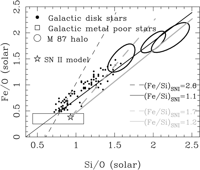
Figure 17: The Fe/O ratio is plotted against the Si/O ratio. Those of disk stars (Edvardsson et al. 1993; closed circles) and average values of metal poor stars (Clementini et al. 1999; open square) in the Galaxy are also plotted. The black solid line and dashed line represent the relation of the abundance pattern with (Fe/Si)_SNIa =1.1 solar (best fit relation) and (Fe/Si)_SNIa=2.6 solar (W7 ratio; Nomoto et al. 1984), respectively. The gray solid line and dashed line represent the relation of (Fe/Si)_SNIa=1.2 and 1.7 solar, respectively, adopting the abundance pattern of the SN II by Iwamoto et al (1999; asterisk) using the nucleosynthesis model of Nomoto et al. (1997) and assuming a Salpeter IMF.

Figure 18: [Mg/O], and [Ca/Si] are plotted against [Fe/O]. Those of disk stars (Edvardsson et al. 1993; closed circles) in the Galaxy are also plotted.

7.3 Nucleosynthesis from SN Ia

The observed radial change of the O/Fe ratio indicates that the contribution from SN Ia increases toward center.

Although the abundance pattern of ejecta of SN II may differ between early-type and late-type galaxies, and that of SN Ia also may not be a constant (Umeda et al. 1999; Finoguenov et al. 2002), for a first attempt we have assumed (Fe/Si)_SNIa, (Si/O)_SNII, and (Fe/O)_SNII to be constants. Here, (Fe/Si)_SNIa is the Fe/Si ratio of ejecta of SN Ia, and (Si/O)_SNII and (Fe/O)_SNII are the Si/O ratio and the Fe/O ratio of the ejecta of SN II, respectively. Since O is not synthesized by SN Ia, the Fe/O ratio is then expressed by,

$$\frac{\rm{Fe}}{\rm{O}}=\left(\rm{\frac{Fe}{Si}}\right)_{\rm{SNIa}}\left(\left(\frac{\rm{Si}}{\rm{O}}\right)-\left(\rm{\frac{Si}{O}}\right)_{\rm{SNII}}\right)+\left(\rm{\frac{Fe}{O}}\right)_{\rm{SNII}}$$ (1)

Thus, (Fe/Si)_SNIa is the inclination in the Si/O vs. Fe/O plot (Figure 17). Even within the M 87 data, the gradient indicates that (Fe/Si)_SNIa at the center is smaller than $\sim$ 1.3 solar. When we adopt the abundance pattern of the Galactic metal poor stars by Clementini et al. (1999) as that of SN II, (Fe/Si)_SNIa around M 87 is determined to be $\sim 1.1$ solar (Table 5 ). In addition, the M 87 data are located at the extension of those of Galactic stars, and the whole trend is consistent with (Fe/Si)_SNIa to be $\sim$ 1.1 solar. This means that also for metal rich stars in the Galaxy, the (Fe/Si)_SNIa is determined to be $\sim$ 1.3 solar. These values are a factor of 2 smaller than the standard W7 model (Nomoto et al. 1984; Table 5), and closer to the WDD1 ratio (Iwamoto et al. 1999), which considers slow deflagration.

In the same way, we have fitted the S and Ar to Si ratio (Figure 19) and derived the S/Si and Ar/Si ratio of SN Ia ((S/Si)_SNIa and (Ar/Si)_SNIa) to be $\sim$ 1.5 solar and 1.3 solar, respectively (Table 5). In contrast to the Fe/Si ratio, W7 and WDDs give nearly the same values for the ratio between the intermediate elements, S/Si and Ar/Si, and the observed ratios are slightly larger than the theoretical values.

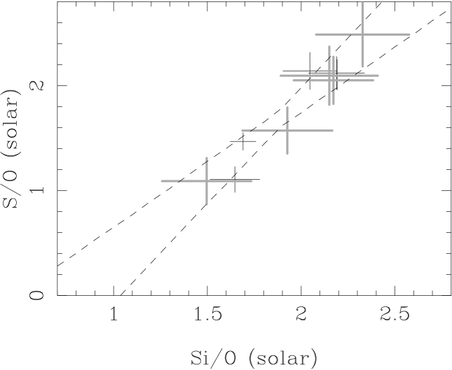
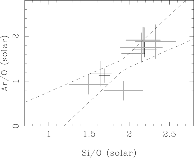
Figure 19: The S/O and Ar/O ratio are plotted against the Si/O ratio observed by the EMOS (black) and the EPN (gray). Dashed lines represents the average relation with 90% significance.

Table 5: The abundance pattern of SN Ia obtained from the ICM of M 87 and those from the nucleo synthesis model of W7 (Nomoto et al. 1984) and WDDs (Iwamoto et al. 1999).

	M 87 SNI	W7	WDD1	WDD2	WDD3
S/Si	1.57$\pm 0.32$	1.05	1.14	1.14	1.14
Ar/Si	1.25$\pm 0.45$	0.76	0.89	0.91	0.93
Fe/Si	1.10$\pm 0.25$	2.61	1.34	2.07	2.99

7.4 Diversity of abundance pattern in SN Ia?

The light curves of observed SN Ia are not identical but display a considerable variation (e.g. Hamuy et al. 1996). In SN Ia, the mass of synthesized Ni⁵⁶ determines the luminosity of each SN. Since the mass of the progenitor should be constant at 1.4 $M_{\odot}$, the ratio of mass of intermediate group elements from Si to Ca, to the mass of Fe and Ni, should depend on the luminosity of SN Ia. The observed luminosity of SN Ia correlates with the type of the host galaxy, and is suggested to be related to the age of the system; SNe Ia in old stellar system may have smaller luminosities (Iwanov et al. 2000), and hence are suggested to yield a smaller Fe/Si ratio (e.g. Umeda et al. 1999).

As discussed in Finoguenov et al. (2002), the smaller Fe/Si ratio observed for the ICM around M 87 may reflect the fact that M 87 is an old stellar system. When we compare the SN Ia abundance pattern for the central and outer regions of M 87, the outer zone SN Ia abundance pattern depends more heavily on the adopted abundance pattern of SN II. As in Finoguenov et al. (2002), we use the SN II pattern derived in Iwamoto et al. (1999) for which a Salpeter IMF was adopted. As indicated in Figure 17, the (Fe/Si)_SNIa of the outer region is determined to be $\sim$ 1.7 solar, while the central region data yield a value of $\sim$ 1.2 solar (Figure 17). In contrast, when we adopt the abundance pattern of metal poor Galactic stars as a SN II pattern, the difference of (Fe/Si)_SNIa of the central and outer regions becomes smaller. The average products of SN II may also differ between the ICM and late-type galaxies, since the IMF of stars may differ between early-type and late-type galaxies. Therefore, (Fe/Si)_SNIa of the outer region still has some uncertainty, while the central value is determined to be $\sim 1.2$ solar, which is not affected by the adopted SN II pattern very much.

However, the metal poor stars, i.e. those with lower Fe/O, tend to be located around larger (Fe/Si)_SNIa values (Figure 17). This result suggests that the SN Ia were dominated by those with larger (Fe/Si)_SNIa when the Galaxy was a young stellar system. Furthermore, based on the ASCA survey of the Virgo cluster, Shibata et al. (2002) discovered that the Fe/Si ratio becomes larger at $R>30^{\prime}$, where the SN Ia products are accumulated from high $z$. Although the O abundance cannot be measured, this result may reflect the fact that the Fe/Si ratio in SN Ia depends on the age of the system.

The ICM in the central and outer regions should have a different origin of metals. As discussed in Paper I, considering the gas mass and stellar mass loss rate, most of the Si and Fe at the center come from present SN Ia in M 87 in the last few Gyr. In contrast, in the outer regions, metals from SN Ia in M 87 are accumulated over a longer time scale, and in addition, other galaxies should contribute to the metals. Since the SN Ia rate is expected to be much larger in the past (Renzini et al. 1993), the SN Ia ejecta which occurred in much younger systems should be important in the outer region.

The indication that the abundance pattern of SN Ia in the outer region of M 87 features a larger (Fe/Si)_SNIa ratio compared to the inner region as found above, can nicely interpreted in line with of these previous findings. The larger (Fe/Si)_SNIa ratio originates from a younger stellar population, so SN Ia products that have been produced earlier in the history of M 87 and the Virgo cluster are more widely distributed in the ICM.

7.5 Nucleo synthesis from SN II

We can also constrain the abundance pattern of SN II in the ICM.

Since Mg and O are not synthesized by SN Ia, the Mg/O ratio reflects those of the products of SN II. The observed Mg/O ratio of $\sim$1.25 solar at $r>0.5^{\prime}$ derived from the line ratio agrees well with that of the Galactic stars, although a higher Mg/O ratio is also allowed within $r<0.5^{\prime}$ due to the uncertainties in the temperature component below 1 keV. This value is also quite similar to the Mg/O ratio of 1.3$\pm 0.2$ solar of the ISM of an X-ray luminous elliptical galaxy, derived from the RGS data (Xu et al. 2002). The central Mg/O reflects the stellar abundance ratio of M 87, while that of outer region is the ratio of of metals in the ICM which is an accumulation of old SN II products ejected from galaxies. Therefore, at least for the Mg/O ratio, there is no observable difference in nucleosynthesis products of SN II between the elliptical galaxies, M 87 and NGC 4636, the ICM and the Galaxy.

The observed S/Si ratio decreases when the O/Si ratio increases (Figure 8, 19). Considering that the observed Fe/Si ratio is constant, this indicates that S/Si ratio is anti-correlated to the O/Fe ratio, that is the contribution from SN II/SN Ia. From equation (1), using S instead of Fe, the S/O ratio in ejecta of SN II ((S/O)_SNII) is obtained from the observed relation in Figure 19. The Si/O ratio of metal poor stars by Clementini et al. (1999) is $\sim 0.7$ solar, while the nucleo synthesis model by Iwamoto et al. (1999) gives the value of 0.9 solar. Therefore assuming that (Si/O)_SNII is less than 1 solar, the extension of the observed values in Figure 19 gives (S/O)_SNII less than 0.5 solar. In the same way, (Ar/O)_SNII is derived to be less than 1 solar.

The observed S abundances of Galactic stars are generally consistent with the Si abundances (e.g. Chen et al. 2002, Takeda-Hidai et al. 2002), although S lines are very week. In contrast, the observation of type II planetary nebulae yielded a S/O and Ar/O ratio to be 0.4$\pm 0.2$ solar and 1.1$\pm 0.5$ solar (Kwitter & Henry 2001). The nucleosynthesis model of SN II by Nomoto et al. (1997) assuming Salpeter’s IMF gives the S/O ratio of 0.6 solar, while another model by Woosley & Weaver (1995) gives a larger ratio of 1 solar. Thus, there may be some uncertainty in the S/O ratio synthesized by SN II even in the Galaxy, and it is also not clear that the Galaxy and the ICM have the same ratio. The fact that the S/Si ratio of the ICM observed with ASCA generally decreases toward outer radius (Finoguenov et al. 2000) supports the low S/Si ratio in SN II, although ASCA cannot constrain O abundance. Therefore, it is important to study outer regions of clusters with the XMM-Newton where SN II may become dominant (e.g. Fukazawa et al. 2000, Finoguenov et al. 2000).

In summary, the SN II abundance pattern observed from the ICM mostly agrees well with that of our Galaxy. Since the abundance pattern of SN II depends on the IMF of stars, this consistency is able to provide strong constraints on it.

7.6 Comparison with the stellar metallicity profile

Figure 20 shows the observed Mg profile, with the stellar metallicity profile from the Mg₂ index (Kobayashi & Arimoto 1999). In addition to the Mg abundance profile derived from the APEC model fit, that from the Mg/Si line ratio and deprojected Si abundance profile is also plotted. The Mg abundance profile of the ICM has a slightly smaller normalization by 20$\sim$30% than the stellar metallicity profile at the same radius.

Although the Mg abundance may have some uncertainties due to the Fe-L atomic data, the APEC code can well fit the Fe-L/Mg-K structure. The uncertainty of the Mg abundance due to the uncertainty of the temperature structure should be also small, at least at $R$=0.5–2^′, since the three temperature model does not change the result, although the abundances from the two- and single-temperature results differ by a factor of 1.5–2. Considering these uncertainties and the difference in observational techniques, we can conclude that the Mg abundance of the ICM is consistent with the stellar metallicity profile at the same radius. Since we are comparing abundances in two distinct media, stars and ISM, which could have very different histories, the abundance results do not have to agree in general. But this agreement is consistent with the picture where the central gas in M 87 comes from stellar mass loss as discussed below.

Figure 20: Mg abundance profile of the EMOS data derived from the spectral fitting with the APEC code (diamonds) and from line ratios (crosses). The dashed line represents the stellar metallicity derived from Mg₂ index (Kobayashi & Arimoto 2000)

7.7 The SN Ia rate of M 87

The metals in the ICM are a sum of metals ejected from the galaxy and those contained previously within the ICM. The observed Fe abundance becomes nearly constant within 2^′, which indicates that the gas is dominated by gas ejected from the galaxy. The observed Mg and Fe abundances within 0.35–2^′ are $1.1\pm 0.2$ solar and 1.54$\pm 0.1$ solar, respectively. Both the nucleosynthesis model by Nomoto et al. (1997) and observation of Galactic stars (e.g. Clementini et al. 1999; Nissen et al. 1994) indicate that (Fe/Mg)_SNII is 0.3–0.5 solar. Therefore, within $R<2^{\prime}$, the Fe abundance synthesized by SN II should be 0.3–0.6 solar. Subtracting it, the Fe abundance synthesized by SN Ia is derived to be $\sim$ 0.9–1.4 solar.

The metallicity of gas ejected from the galaxy are a sum of stellar metallicity and the contribution from SN Ia, and can be expressed as,

$$z^{i}=\frac{\alpha_{*}y^{i}_{*}+\alpha_{\rm SN}y_{\rm SN}^{i}}{\alpha_{*}+\alpha_{\rm SN}}\sim y_{*}^{i}+\langle\frac{\alpha_{\rm SN}}{\alpha_{*}}\rangle y_{\rm SN}^{i}$$

$$=y_{*}^{i}+\langle\frac{\theta_{\rm SN}M_{\rm SN}^{i}}{\alpha_{*}}\rangle$$ (2)

(Loewenstein and Mathews 1991; Ciotti et al. 1991), where $z^{i}$ is the mass fraction of the $i$th element, $\alpha_{*}$ and $\alpha_{\rm SN}$ are the mass loss rates of stars and SNe respectively, and $y_{*}^{i}$ and $y_{\rm SN}^{i}$ are their yields. $\theta_{\rm SN}$ is the SN Ia rate and $M_{\rm SN}^{i}$ is the mass of the $i$th element synthesized by one SN Ia. Converting to abundance in unit of the solar ratio, Fe abundance synthesized by SN Ia of gas ejected from an elliptical galaxy becomes

$${{{A_{*}^{\rm{Fe}}}_{\rm SNIa}}}+\left(\frac{\theta_{\rm SN}\rm M_{\rm SN}^{\rm Fe}}{\alpha_{*}}\right)\left(z^{\rm Fe}_{\rm solar}\right)^{-1}$$

$$={{{A_{*}^{\rm{Fe}}}_{\rm SNIa}}}+2.1\frac{{\left(\frac{\theta_{\rm SN}}{1.0\times 10^{-13}/{\rm yr}/L_{\rm B}}\right)}\left(\frac{M^{\rm Fe}_{\rm SN}}{0.4M_{\odot}}\right)}{{\left(\frac{\alpha_{*}}{1.5\times 10^{-11}M_{\odot}/{\rm yr}/L_{\rm B}}\right)}}$$ (3)

Here, ${{{A_{*}^{\rm{Fe}}}_{\rm SNIa}}}$ is stellar Fe abundance synthesized by SN Ia and $M^{\rm Fe}_{\rm SN}$ is the mass of Fe synthesized by one SN Ia. $z^{\rm Fe}_{\rm solar}$ is the Fe metallicity of gas with the solar abundance. Considering the fact that recent observations of M 87 and A 496 (Tamura et al. 2001) indicate a smaller Fe/Si ratio synthesized by SN Ia than usually assumed previously, $M_{\rm Fe}$ of one SN Ia should be $\sim 0.4M_{\odot}$. From a theoretical stellar evolutionally model for a stellar population, the stellar mass loss rate is approximated by $1.5\times 10^{-11}L_{B}t_{15}^{-1.3}M_{\odot}/yr$, where $t_{15}$ is the age in unit of 15 Gyr, and $L_{B}$ is the B-band luminosity (Ciotti et al. 1991). An infrared observation, which can directly trace mass loss rate from asymptotic giant branch stars, gives a consistent value within a factor of 2 with the theoretical value (Athey et al. 2002). The SN Ia rate of elliptical galaxies is estimated to be 0.13$\pm$0.05 ${h_{75}}^{2}$ SN Ia/100yr/10${}^{10}L_{\odot}$ (Cappellaro et al. 1997). Here, $h_{75}$ is a Hubble constant in unit of 75 km s^-1 Mpc^-1. Using the Hubble constant of 72$\pm 8$ km s^-1 Mpc^-1 (Freedman et al. 2001), the present contribution from SN Ia to the Fe abundance becomes 1.4–3.6 solar.

Considering the large error due to a statistical error and uncertainties in bias corrections of SN Ia from optical observation, this value is consistent with the Fe abundance synthesized by SN Ia within 2^′, 0.9–1.4 solar, which is a sum of ejecta of present SN Ia and that was trapped in stars and comes from stellar mass loss. The contribution from stars to Fe synthesized by SN Ia may be small, since stars in giant elliptical galaxies are thought to have a SN II like abundance pattern (e.g. Worthey et al. 1993).

7.8 Implication of S abundance

In Sec.7.5 we indicated that the S/Si ratio in SN II is much lower than 1 solar. If this fact is valid universally in the ICM, then the S/Si ratio may be a better indicator for the contribution from the SN Ia/SN II than the Fe/Si ratio. Of course, the best indicators of SN II are O, Ne and Mg, which are not synthesized in SN Ia. However, emission lines of Ne and Mg are often hidden in the strong Fe-L lines, and the O abundance can be measured only in relatively cool clusters.

As discussed in Sec.7.4 the Fe/Si ratio of SN Ia may be expected to show a variation, since the luminosity of the SN Ia should reflect the amount of Ni⁵⁶ synthesized by SN Ia. The pure SN II ejecta may provide the smaller Fe/Si ratio. Then SN Ia in young systems occur, which may have a larger Fe/Si ratio and so the Fe/Si ratio increases. Finally, SN Ia in old systems decrease the Fe/Si ratio again. In contrast, at least in Iwamoto et al. (1999), the S/Si ratio in the various SN Ia is almost constant. In addition, as shown in Sec. 5.2, the S/Si line ratio does not depend on the plasma temperature, while that of the Fe/Si is a very strong function. This means that, the derived S/Si does not depend on the temperature structure of the ICM. This is a very important advantage for the cool cores of the cluster center, where many temperature components exists.

The problem is that both Si and S are synthesized in the same nucleo process, i. e. in the same region in the SN. Therefore, it is surprising that the S/Si ratio shows a radial variation. Unfortunately, the S abundance measured of the Galactic stars has very large uncertainties, and the S/Si ratio of the SN II may also depend on the IMF of stars. Therefore, it is quite important to calibrate the S/Si vs. O/Fe pattern in luminous clusters.

8 Summary and Conclusion

Based on the temperature structure studied in Paper I, abundance profiles of 7 elements of the ICM around M 87 are obtained using the deprojected spectra. We have discussed the use of one- and two-temperature models in the fit and the application of the MEKAL and APEC codes. Two temperature models are only important in the region, R$<2$ arcmin. The previous problems with an earlier version of the APEC code are now resolved in the present version and this code provides now better fitting solutions in general. In addition, using line ratio profiles of the projected and deprojected data, the abundance ratio profiles are obtained with smaller uncertainties, considering the temperature dependence of the line ratio, The main results obtained are as follows,

• Abundance profiles of 7 elements are obtained with high accuracy (e.g. $\delta$Fe$\sim\delta$Si$\sim$5%, $\delta$O$\sim$10%).

• The Si and Fe abundance profiles have steep gradients at $>2^{\prime}$ with a Fe/Si ratio of $0.9\pm 0.1$ solar, and become constant within this radius at 1.5–1.7 solar.

• The S/Si ratio is about 1 solar at $r<$ 4^′ and decreases to $\sim$ 0.7 solar at $r>10^{\prime}$.

• The Ar/Si and Ca/Si are about 0.8 solar and 1.5 solar, respectively, although errors are relatively large.

• The O and Mg abundances are smaller than the abundances of Fe and the intermediate elements. The O/Si ratio is less than half solar at the center and increases with radius. The Mg/O ratio is 1.25 solar and consistent with no radial gradients at least at $r>0.5^{\prime}$.

• The observed abundance pattern among O, Mg, Si, Ca and Fe of the ICM is located at an extension of that of Galactic stars. Therefore, the abundance pattern of the ICM is not peculiar and it should strongly constrain the products of SN Ia and SN II of early-type and late-type galaxies.

• The Si/O/Fe diagnostics shows large Si contributions by SN Ia, which may reflect the observational finding that SN Ia in old stellar systems are fainter.

• The observed Mg abundance of the ICM is consistent with the stellar metallicity profile from the Mg₂ index at the same radius. This result is consistent with stellar mass loss as the source of the gas in the very central region of M 87.

• The central abundance can be explained with the observed SN Ia rate and SN Ia model yields.

• The different radial profiles between Si and S suggest that the S/Si ratio synthesized from SN II is much smaller than the solar ratio. Then, the S/Si ratio may be a better indicator of the relative contribution from SN Ia and SN II, when O and Mg abundances cannot be observed.

We are actually very fortunate to have M 87 and the Virgo cluster as the closest galaxy cluster in our neighborhood, since it offers an ICM in just this low temperature range where the spectra are richest in spectral lines for this type of abundance diagnostics. Therefore it would be worthwhile to use this unique case for even deeper observations and more detailed investigations by X-ray spectroscopy in the future.

- (1) Anders E., & Grevesse N., 1989, Geochim. Cosmochim. Acta, 53,197
- (2) Arnaud M., Rothenflug R., Boulade O., et al. 1992, A&A, 254, 49
- (3) Athey A., Bregman,J., Bregman J., & Temi, P. 2002, ApJ, 571, 272
- (4) Belsole E., Sauvageot, J.L., Böhringer, H., et al. 2001, A&A, 365, L188
- (5) Böhringer H., Nulsen P.E.J., Braun R., & Fabian A.C., 1995, MNRAS, 274, 67
- (6) Böhringer, H., Belsole, E., Kennea, J., et al. 2001, A&A, 365, L181
- (7) Cappellaro E., Turatto M.; Tsvetkov, D. Yu.; Bartunov O. S.; Pollas C.; Evans R.; Hamuy M., 1997, A&A, 322, 431
- (8) Chen Y.Q., Nissen, P.E., Zhao, G.,& Asplund, M., 2002, A&A, 390, 225
- (9) Clementini, G., Gratton, R.G., Carretta, E., & Sneden, C, 1999, MNRAS, 302, 22
- (10) Ciotti L., Pellegrini S., Renzini A., & D’Ercole A. 1991, ApJ, 376, 380
- (11) Edvardsson, E., Andersen, J., Gustafsson B., et al. 1993, 275, 101
- (12) Fabian A.C., et al. 1984, Nature, 307, 343
- (13) Feldman, U., 1992, Physica Scripta 46, 202
- (14) Finoguenov, A., David, L.P., & Ponman, T.J, 2000, ApJ, 544, 188
- (15) Finoguenov A., Matsushita, K., Böhringer, H., et al. 2002, A&A 381, 21
- (16) Freyberg, M. J., Briel, U.G., Dennerl, K., Haberl, F., Hartner, G., Kendziorra, E., Kirsch M., 2002, in Symp. New Visions of the X-ray Universe in the XMM-Newton and Chandra Era (ESA SP-488; Noordwijk: ESA)
- (17) Freedman, W. L., Madore, B.F., Gibson, B.K., et al. 2001, ApJ, 553, 47
- (18) Fukazawa, Y., Makishima, K., Tamura, T., et al. 1998, PASJ, 50, 187
- (19) Fukazawa, Y., Makishima, K., Tamura, T., et al. 2000, MNRAS, 313, 21
- (20) Gastaldello, F., & Molendi, S., 2002, ApJ, 572, 160
- (21) Gratton, R.G., & Sneden, C., 1991, A&A, 241, 501
- (22) Hamuy, M., Philips, M.M., Suntzeff, N.B., et al. 1996, AJ, 112, 2438
- (23) Iwamoto, K., Brachwitz, F., Nomoto, K., et al. 1999, ApJS, 125,439
- (24) Iwanov, V., Hamuy, M., & Pinto, P.A., 2000, ApJ. 542,588
- (25) Kaastra J.S. 1992, An X-Ray Spectral Code for Optically Thin Plasmas (Internal SRON-Leiden Report, updated version 2.0)
- (26) Katayama, H., Takahashi, I., Ikebe, Y., Matsushita, K., & Freyberg, M., 2002., submitted to A&A (astroph/0210135)
- (27) Kobayashi, C., & Arimoto, N., 1999, ApJ. 527, 573
- (28) Kodama, T., Arimoto, N., Barger, A., et al. 1998, A&A, 334, 99
- (29) Kwitter, K.B., & Henry, R.B.C, 2001, ApJ, 562, 804
- (30) Liedahl D. A., Osterheld A.L., & Goldstein W.H. 1995, ApJ, 438, L115
- (31) Loewenstein M., & Mathews W.G. 1991, ApJ, 373, 445
- (32) Masai K. 1997, A&A, 324, 410
- (33) Matsushita, K., Makishima, K., Rokudanda, E., Yamasaki, N. Y., & Ohashi, T., 1997, ApJ, 488, 125
- (34) Matsushita K., Ohashi T., & Makishima K., 2000, PASJ, 52, 685
- (35) Matsushita, K., Belsole, E., Finoguenov, A., & Böhringer, H., 2002, A&A, 386, 77 (Paper I)
- (36) Mewe R., Gronenschild E.H.B.M., & van den Oord G.H.J. 1985, A&AS, 62,197
- (37) Mewe R., Lemen J.R., & van den Oord, G.H.J. 1986, A&AS, 65,511
- (38) Mushotzky, R., Loewenstein, M., Arnaue, K.A., et al. 1996, ApJ, 466
- (39) Nissen, P.E., Gustafsson, B., Edvardsson, B., et al. 1994, A&A, 285, 440
- (40) Nomoto, K., Thielemann, F-K., & Wheeler, J.C., 1984, ApJ, 279, 23
- (41) Nomoto, K., Hashimoto, M., Tsujimoto, T., et al. 1997, Nuclear Physics A., 616, 79
- (42) Peimbert, M., 1992, in Elements and the Cosmos, ed. M.G.Edmunds & R.J. Terlevich (Cambridge: Cambridge Univ. Press), 196
- (43) Renzini A., Ciotti, L., D’Ercole, A., & Pellegrini, S. 1993, ApJ, 419, 52
- (44) Sakelliou, I., Peterson, J.R., Tamura, T., et al. 2002, A&A, 391, 903
- (45) Smith, R.K., Brickhouse, N.S., Liedahl,D.A., & Raymond, J.S., 2001, ApJ, 556, 91
- (46) Shibata, R., Matsushita, K., Yamasaki, N.Y., et al. 2001, ApJ, 549, 228
- (47) Shibata, R., Matsushita, K.,. Yamasaki, N.Y., et al. 2002, in preperation
- (48) Shigeyama T., 1998, ApJ, 497, 587
- (49) Stanford, S. A., Eisenhardt, P. R. M., & Dickinson, M., 1995, ApJ, 450, 512
- (50) Takeda-Hidai, M., Sato, S., Honda, S., et al. 2002, ApJ, 573, 614
- (51) Tamura, T., Bleeker, J.A.M., Kaastra, J.S, et al. 2001, A&A, 379, 107
- (52) Thielemann, F-K., Nomoto, K., & Hashimoto, M. 1996, ApJ, 460, 408
- (53) Umeda H., Nomoto K., & Kobayashi C. 1999, ApJ, 522, L43
- (54) Woosley, S.E., & Weaver, T.A., 1995, ApJS, 101, 181
- (55) Worthey, G., Faber, S.M., & González, J.J. 1992, ApJ, 398, 69
- (56) Xu, H., Kahn, S., Peterson, J.R., Beher E., Paerels, F.B.S., Mushotzky, R. F., Jernigan, J.G., & Makishima, K., 2002, ApJ, 579, 600