Abstract

A technique of timescale analysis performed directly in the time domain has been developed recently. We have applied the technique to study rapid variabilities of hard X-rays from neutron star and black hole binaries, $\gamma$-ray bursts and terrestrial $\gamma$-ray flashes. The results indicate that the time domain method of spectral analysis is a powerful tool in revealing the underlying physics in high-energy processes in objects.

[Timescale Spectra in High Energy Astrophysics] Timescale Spectra
in High Energy Astrophysics

1 Introduction

The widely used Fourier analysis method in temporal analysis is to derive frequency spectra from a time series. After the Fourier transform of a light curve $x(t_{k})$

$$X(f_{j})=\sum_{k}x(t_{k})e^{-i2\pi f_{j}k\Delta t},\hskip 14.22636ptf_{j}=j/T$$ (1)

we can get the power density spectrum

$$P_{j}=|X(f_{j})|^{2}$$ (2)

From two light curves, $x_{1}(t_{k})$ and $x_{2}(t_{k})$, observed simultaneously in two energy bands at times $t_{k}$, and their Fourier transforms $X_{1}(f_{j})$ and $X_{2}(f_{j})$, we can construct the cross spectrum

$$C(f_{j})=X_{1}^{*}(f_{j})X_{2}(f_{j})$$ (3)

and then the time lag spectrum

$$\Lambda(f_{j})=\arg[C(f_{j})]/2\pi f_{j}$$ (4)

and the coherence coefficient spectrum

$$r(f)=\frac{|<C(f)>|}{\sqrt{<|X_{1}(f)|^{2}><|X_{2}(f)|^{2}>}}$$ (5)

People usually take a Fourier period $1/f$ as a timescale and use the Fourier power spectrum to describe the distribution of variation amplitude at different timescales, the time lag spectrum to describe the distribution of the emission time difference between two energy bands at different timescales and the coherence coefficient spectrum to describe the distribution of degree of linear correlation between high and low energy processes at different timescales. But it is not correct to equate the Fourier period with the timescale; a Fourier component with a certain frequency $f$ of a light curve is not equal to the real process with the timescale $1/f$. For some important high-energy emission processes the Fourier spectra distort the timescale distribution of real physical processes seriously. It is needed to derive timescale spectra from observed light curves directly in the time domain without through Fourier transforms.

2 Power Spectra

The power density spectrum can be derived directly in the time domain (Li 2001). For a counting series $x(k),~{}k=1,...,N$ obtained from a time history of observed photons with a time step $\Delta t$, the definition of variation power is

$$P(\Delta t)=\frac{\mbox{Var}(x)}{(\Delta t)^{2}}=\frac{\frac{1}{N}\sum_{k=1}^{N}(x(k)-\bar{x})^{2}}{(\Delta t)^{2}}=\frac{1}{N}\sum_{k=1}^{N}(r(k)-\bar{r})^{2}\hskip 8.53581pt\mbox{rms${}^{2}$}$$ (6)

where $r=x/\Delta t$. The power density $p(\Delta t)$ at a timescale $\Delta t$ can be then derived

$$p(\Delta t)=\frac{\mbox{d}P(\Delta t)}{\mbox{d}\Delta t}\simeq\frac{P(\Delta t_{1})-P(\Delta t_{2})}{\Delta t_{2}-\Delta t_{1}}\hskip 19.91692pt\mbox{rms${}^{2}$/s}$$ (7)

From (6), (7) we can calculate the power density for Poison noise

$$p_{noise}(\Delta t)\simeq\frac{r}{\Delta t_{1}\Delta t_{2}}\hskip 19.91692pt\mbox{rms${}^{2}$/s}$$ (8)

and the signal power density can be defined as

$$p_{signal}(\Delta t)=p(\Delta t)-p_{noise}(\Delta t)\hskip 19.91692pt\mbox{rms${}^{2}$/s}$$ (9)

Distribution of power density vs. time scale of a shot model. Top panel: the signal, stochastic exponential shots with time constant $\tau$ between 5 ms and 0.2 s. Middle panel: simulated data which involved both signal and Poisson noises. Bottom panel: signal power densities . Solid line – power density distribution of time scale expected for the signal. Dashed line – excess Fourier spectrum from the simulated data. Plus signs – excess power densities calculated by the timing technique in the time domain for the simulated data.

In Fig. 1 the bottom panel shows the expected power spectrum (solid line) for a signal consisting of stochastic shots (shown in the top panel), the timescale spectrum of power density (crosses) and Fourier spectrum (dashed line) from the simulated data (shown in the middle panel) of the stochastic signal. As the rise and decay time constant of a shot is randomly taken from the range between 5 ms and 0.2 s, there should exist significant variation power in this timescale region. One can see from Fig. 1 that the Fourier spectrum significantly underestimates the power densities at the shorter timescales.

Timescale spectra of power density can help to reveal the nature of physical process around compact stars (Li & Muraki 2002). Figure 2 shows the timescale spectra and Fourier spectra of power density for a sample of accreting black holes (left side) and neutron stars (right side). The five black hole candidates demonstrate a significant power excess in the timescale spectra in comparison with their corresponding Fourier spectra at timescales shorter than $\sim 0.1$ s, but the two kinds of power spectrum in the studied neutron stars are generally consistent with each other. Assuming that there exist a stochastic process with a characteristic time of $\sim 0.1$ s in the black hole systems and that a significant variability of the accreting neutron stars comes from stochastic processes with characteristic time constants much shorter than $\sim 1$ ms can explain the observed power spectra for X-ray binaries.

Figure 1: Power density vs. timescale of black hole binaries (left side) and neutron star binaries (right side). $Crosses$: Timescale spectra. $Dots$: Fourier spectra

3 Time Lag Spectra

Measuring the relative time delay between photons in two energy bands can give useful clue to understanding the emission mechanism and emitting region (e.g., Kazanas, Hua & Titarchuk 1997; Hua, Kazanas & Titarchuk 1997; Nowak et al. 1999). With the cross-correlation analysis one can calculate a time lag $\Lambda$ from two light curves. Traditional cross-correlation method fails to calculate any time lag shorter than the time step $\Delta t$. In studying a complex process only a time lag $\Lambda$ is not enough, we need to know time lags at different timescales, i.e. the timescale spectrum $\Lambda(\Delta t)$. Using Fourier analysis we can get a time lag spectrum. But as the Fourier technique is powerless for detecting the variation power of a stochastic process at high frequencies (short timescales) range, the Fourier analysis method is also powerless for detecting the time lags at high frequencies (short timescales).

The timescale spectrum of time lag can be derived with a modified cross-correlation technique (Li, Feng & Chen 1999; Li 2001). For two light curves $x_{1}(k),~{}x_{2}(k)$ with a time step $\Delta t$ the modified cross-correlation function at $\tau$ is defined as

$$\mbox{C}(\tau;\Delta t)=\sum_{k}v_{1}(k\Delta t)v_{2}(k\Delta t+\tau)/\sigma(v_{1})\sigma(v_{2})$$ (10)

where $v(t)=x(t)-\bar{x}$, $\sigma^{2}(v)=\sum v^{2}$, $x(t)$ is the counts in the time interval $(t,t+\Delta t)$. Find the time lag $\Lambda$ letting $C(\tau=\Lambda;\Delta t)=\max$ for different timescale $\Delta t$, we can derive the timescale spectrum of time lag, $\Lambda(\Delta)$.

For comparing the two kinds of spectrum for time lags, timescale spectrum and Fourier spectrum, we construct two simulated time event series which consist of two kinds of random shot component : rapid components with typical timescale 1 ms and time lag 5 ms and slow component with timescale 0.01 s and time lag 0.02 s. Figure 3 shows that the timescale spectrum can represent the time delay distribution in the real process, but the Fourier analysis is powerless to detecting the time lags in the short timescale range.

Time lags between two series of events $\{t\}$ and $\{t^{\prime}\}$. Each series consists of three components. $\{t\}=\{x\}+\{y\}+\{z\},\{t^{\prime}\}=\{x^{\prime}\}+\{y^{\prime}\}+\{z^{\prime}\}$. The first random shot component $\{x\}$ and $\{x^{\prime}\}$ have exponentially rising and decay time $\tau=0.01$ s and $x^{\prime}(i)=x(i)+0.02$s. The second random shot component $\{y\}$ and $\{y^{\prime}\}$ have exponentially rising and decay time $\tau=1$ ms and $y^{\prime}(i)=y(i)+5$ms. Total shot rate is 1000 cts/s. $\{z\}$ and $\{z^{\prime}\}$ are two independent white noise series with rate of 100 cts/s. The series duration is 2000 s. $Crosses$ are from the time domain technique, $Circles$ from the Fourier analysis.

The timescale spectral method for time lag analysis is a powerful tool in revealing the characteristic of emission process. Applying the time domain technique, Qu et al. (2001) detected time lags of hard X-ray photons from Cyg X-1 in the short timescale region ($\Delta t<0.01$ s or $f>100$ Hz) with PCA/RXTE data for the first time, giving strong constraint on emission mechanism; Feng et al. (2002) revealed the time delays of soft photons in terrestrial gamma-ray flashes (TGFs) observed by BATSE/CGRO, strongly supporting the discharging mechanism of TGF production. Investigating temporal properties of GRBs by the timescale spectral method is in process. Figure 4 shows the spectrum of time lag of soft photons and the energy dependence of time lag for GRB910503 detected by BATSE.

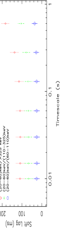
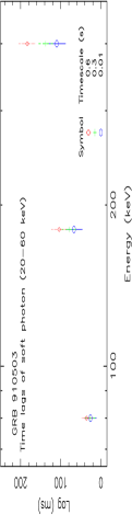
Figure 2: Soft time lags of GRB 910503. $Left~{}panel$: Timescale spectra of time lag. $Right~{}panel$: Time lag of 20-60 keV photons vs. energy of hard photons.

4 Discussion

The complex variability of high-energy emission shown in different time scales is a common character for X-ray binaries, super massive black holes and $\gamma$-ray bursts. The variability is caused by various physical processes at different timescales. For understanding the emission process of high-energy photons it is necessary to know the variation characteristics in different timescales quantitatively, i.e. to derive timescale spectra from observed light curves. In addition to the methods of making spectral analysis for power density and time lag in the time domain introduced in last two sections, the algorithms to calculate timescale spectra for coherence, hardness, variability duration, and correlation coefficient between two characteristic quantities have been also proposed (Li 2001).

There now exist two kinds of spectral analysis: frequency analysis and timescale analysis. As any observable physical process always occurs in the time domain, a frequency spectrum obtained by frequency analysis needs to be interpreted in the time domain. But a frequency analysis is based on a certain kind of time-frequency transformation. Different mathematically equivalent representations with different bases or functional coordinates in the frequency domain exist for certain time series, a Fourier spectrum with the trigonometric basis does not necessarily represent the true distribution of a physical process in the time domain. The rms variation vs. timescale of a time-varying process may differ substantially from its Fourier spectrum. Figure 1 shows that the Fourier transform distorts the power density distribution of a stochastic process at short timescales seriously. The timescale analysis performed directly in the time domain can derive real timescale distribution for quantities characterizing temporal property. In comparison with the frequency analysis, timescale spectra from the timescale analysis can more exactly represent timescale distributions of a real physical process, and more sensitively reveal temporal characteristics at short timescales for a stochastic process. Until now Fourier analyses of variabilities of X-ray binaries observed by various instruments are all failure to detect hard X-ray lags at the high frequency region of $f>100$ Hz. Our simulation study shows it is an intrinsic weakness of the Fourier method, that more sensitive X-ray detectors of next generation can still not observe high frequency lags with Fourier technique. On the other hand, the timescale analysis can already derive time lag spectra at short timescales reliably from existing data.

1

References

- [1] Li T.P. (2001) Chin. J. Astron. Astrophys., 1, 313
- [2] Li T.P., Feng Y.X. & Chen L. (1999) ApJ, 521, 789
- [3] Li T.P. & Muraki Y. (2002) ApJ, 578, 374
- [4] Feng H., Li T.P., Wu M., Zha M. & Zhu Q.Q. (2002) , 29, No.3
- [5] Hua X.M., Kazanas D. & Titarchuk L. (1997) , 482, L57
- [6] Kazanas D., Hua X.M. & Titarchuk L. (1997) , 480, 735
- [7] Nowak M.A., Wilms J., Vaughan B.A., Dove J.B. & Begelman C. (1999) , 510, 874
- [8] Qu J.L. & Li T.P. (2001) Acta Astron. Sin., 42, 140