Helical surface structures

Abstract

Over the past few years there has been growing interest in helical magnetic field structures seen at the solar surface, in coronal mass ejections, as well as in the solar wind. Although there is a great deal of randomness in the data, on average the extended structures are mostly left-handed on the northern hemisphere and right-handed on the southern. Surface field structures are also classified as dextral (= right bearing) and sinistral (= left bearing) occurring preferentially in the northern and southern hemispheres respectively. Of particular interest here is a quantitative measurement of the associated emergence rates of helical structures, which translate to magnetic helicity fluxes. In this review, we give a brief survey of what has been found so far and what is expected based on models. Particular emphasis is put on the scale dependence of the associated fields and an attempt is made to estimate the helicity flux of the mean field vs. fluctuating field.

Nordita, Blegdamsvej 17, DK-2100 Copenhagen Ø, Denmark

Department of Physics & Astronomy, University of Rochester, Rochester NY 14627

1. Introduction

There is now good evidence for the helical nature of the solar magnetic field. Early work by Seehafer (1990) suggested that fitting the line of sight magnetograms of solar active regions to a linear (constant alpha) force-free magnetic field yields systematically negative values of alpha in the northern hemisphere and positive in the southern. Although the evidence for the hemispheric dependence was perhaps not completely convincing back then, subsequent work by different groups (Pevtsov, Canfield, & Metcalf 1995; Rust & Kumar 1996; Bao et al. 1999; Pevtsov & Latushko 2000) have confirmed the initial results.

The quantity being measured in these studies is usually the current helicity, $\int{\bf{J}}\cdot{\bf{B}}\,{\rm d}{}V$, or the current helicity density, ${\bf{J}}\cdot{\bf{B}}$, where ${\bf{B}}$ is the magnetic field strength, ${\bf{J}}=\mbox{\boldmath$\nabla$}{}\times{\bf{B}}/\mu_{0}$ is the current density, and $\mu_{0}$ is the magnetic permeability. Of particular interest is actually the magnetic helicity $\int{\bf{A}}\cdot{\bf{B}}\,{\rm d}{}V$, where ${\bf{A}}$ is the magnetic vector potential with ${\bf{B}}=\mbox{\boldmath$\nabla$}{}\times{\bf{A}}$.

The magnetic helicity is of great theoretical interest because it satisfies a conservation law: except for small resistive terms, its rate of change depends only on the gains and losses of magnetic helicity through the boundaries. However, the magnetic helicity is a volume integral which is probably hopeless to measure in practice, because the field cannot be observed in the solar interior. What is possible, however, is to measure surface-integrated magnetic helicity fluxes of the form $\int({\bf{E}}\times{\bf{A}})\cdot{\rm d}{}V$, where ${\bf{E}}={\bf{J}}/\sigma-{\bf{u}}\times{\bf{B}}$ is the electric field and $\sigma$ is the electric conductivity. Regardless of numerous complications, recent work has confirmed the basic hemispheric dependence of the sign of both current helicity densities and surface-integrated magnetic helicity fluxes (Berger & Ruzmaikin 2000, DeVore 2000, Chae 2000): negative in the north and positive in the south.

The connection between current helicity and dynamo theory was immediately recognized. Rädler & Seehafer (1990) proposed that the observed signs of the current helicity are characteristic of the small scale field rather than the large scale field. From a dynamo point of view this is not only plausible, but also desirable, as we shall explain later. From an observational point of view this is far less obvious, because the field on the scale of active regions and that associated with coronal mass ejections (CMEs) is not generally understood as part of the small scale field. Eclipse images of the sun map out quite clearly the overall field line structure (e.g. Fig. 1 in Low 2001). From these one sees that the field lines in helmet streamers above and around CMEs merges naturally with the large scale of the sun. This is also seen in soft X-ray images from Yohkoh (e.g. Fig. 7 in Low 2001).

The purpose of this paper is to point out that, on theoretical grounds, one might expect a certain degree of simultaneous emergence of small and large scale fields of opposite helicities within each hemisphere. (This concept was also discussed in Blackman & Field 2000.) In the following, we explain the reasoning behind such an expectation in light of recent work, and suggest possible observational signatures of the process.

2. Simultaneous production of positive & negative magnetic helicity

Magnetic helicity is being produced by differential rotation and cyclonic convection (the $\alpha$-effect). Both sources of magnetic helicity have been discussed in the past (e.g. Berger & Ruzmaikin 2000). Here we focus on the effect of cyclonic convection ($\alpha$-effect). It is well known that the $\alpha$-effect does not produce any net magnetic helicity (so it obeys magnetic helicity conservation in the limit of large magnetic Reynolds numbers). Instead, it produces simultaneously positive and negative magnetic helicity associated with a spectral segregation (Seehafer 1996, Ji 1999). The question then arises where do each of these oppositely helical contributions of the magnetic field go? There are three possibilities: reconnection across the equator, resistive cancellation, and losses at the solar surface. The latter is by far the most plausible one. What is not so clear is how exactly one is supposed to picture the simultaneous loss of oppositely helical magnetic fields. More importantly, why has there been no observational evidence of this, neither quantitatively nor qualitatively? Recently, however, Démoulin et al. (2002) reported that sufficiently far away from the photospheric inversion line writhe helicity (resulting from the relative rotation of opposite polarities) and twist helicity (resulting from the intrinsic rotation of either polarity) can have different signs. This may well be an indication of the anticipated simultaneous loss of magnetic helicity of both signs.

From a turbulence point of view, one expects that any kind of helical stirring leads to the development of an inverse cascade (Pouquet, Frisch, & Léorat 1976). As is now well established from simulations, this can be seen in power spectra of the magnetic energy: helical forcing at or around some wavenumber $k_{\rm f}$ leads to a spectral bump at $k<k_{\rm f}$ (larger wavelength) where the spectral magnetic helicity is opposite to that at the forcing wavenumber. As time goes on, this bump travels toward smaller $k$, until it reaches the wavenumber corresponding to the scale of the system.

The inverse cascade mechanism and the $\alpha$-effect are similar (but see Brandenburg 2002 for pointing out differences), and they are widely considered to be the most plausible mechanism for explaining the solar magnetic field. In addition to the helicity effect (inverse cascade or $\alpha$-effect), there is also shear (or differential rotation) which amplifies the toroidal magnetic field, regardless of magnetic helicity. A rough measure of the relative importance of shear and helical turbulence can be obtained by considering the ratio of toroidal to poloidal magnetic field. For the sun this ratio is between 10 and 100. For poloidal magnetic field generation, shear does not contribute.

Shear tends to produce large scale magnetic fields that oscillate on a time scale long compared with the turnover time of the turbulence. This result goes back to Parker (1955), and is well understood in the framework of mean-field dynamo theory (Moffatt 1978, Parker 1979, Krause & Rädler 1980, Zeldovich, Ruzmaikin, & Sokoloff 1983), and also confirmed using direct simulations of helical turbulence with sinusoidal shear (Brandenburg, Bigazzi, & Subramanian 2001). In the framework of this model, the long term cycles are to be identified with the 22-year magnetic cycle of the sun. The magnetic field takes the form of traveling waves that migrate in the direction perpendicular to the shear. This migration may be identified with the migration of sunspot belts toward the equator, though under certain circumstances the direction of the field migration can be overturned by meridional circulation (Choudhuri, Schüssler, & Dikpati 1995, Durney 1995, Küker, Rüdiger, & Schultz 2001).

The outer boundaries of the sun do allow magnetic field to escape, but it is not clear just how much magnetic flux really does escape. In simulations of forced hydromagnetic turbulence with open boundaries (pseudo-vacuum boundary conditions) magnetic field is found to escape both on small and large scales, and these two contributions do indeed have opposite signs of magnetic helicity, but the contribution from small scales is found to be weak compared with that from larger scales. It is not entirely clear yet whether the boundary condition is realistic enough and whether the comparatively weak losses of small scale field are representative of the real solar magnetic field.

Before we discuss why small scale losses of helical magnetic fields are important (and even advantageous) for $\alpha$-effect dynamos, we illustrate first how to picture such simultaneous losses of oppositely helical magnetic fields, and what the observable signatures of this process would be.

3. Simultaneous losses of oppositely helical magnetic fields

Given that magnetic helicity is conserved in the absence of boundary losses and resistivity, any swirl-like motion must introduce simultaneously oppositely helical magnetic fields when starting with an initially non-helical magnetic field (Longcope & Klapper 1997). The prime example is of course the formation of an $\Omega$-shaped flux loop due to magnetic or thermal buoyancy, and the simultaneous tilting due to the Coriolis force. This is sketched in Fig. 1.

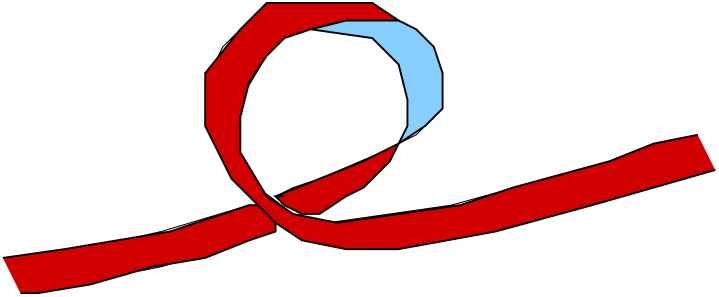
Figure 1.: Tilting of the rising tube due to the Coriolis force. Note that the tilting of the rising loop causes also internal twist.

The tilting of the tube does clearly introduce current helicity, ${\bf{J}}\cdot{\bf{B}}$, where ${\bf{J}}$ is the current density associated with the magnetic loop. The relation between this and the magnetic helicity is not very direct. The resistive driving of the current helicity is proportional to the current helicity,

$${{\rm d}\over{\rm d}t}\int{\bf{A}}\cdot{\bf{B}}\,{\rm d}V=-2\eta\mu_{0}\int{\bf{J}}\cdot{\bf{B}}\,{\rm d}V-\mbox{surface terms},$$ (1)

but apart from this, the only direct relation is between the spectra of magnetic and current helicities, $H(k)$ and $C(k)$, respectively. The spectra are normalized such that

$$\langle{\bf{A}}\cdot{\bf{B}}\rangle=\int_{0}^{\infty}H(k){\rm d}k,$$ (2)

where angular brackets denote volume averages, and

$$\langle{\bf{J}}\cdot{\bf{B}}\rangle=\int_{0}^{\infty}C(k){\rm d}k;$$ (3)

and the two are related to each other simply by

$$\mu_{0}C(k)=k^{2}H(k).$$ (4)

Since $H(k)$ and $C(k)$ can be of either sign, $\int H(k){\rm d}k$ can be of either sign for the same sign of $\int C(k){\rm d}k$ for example. A useful tool is however the two-scale analysis, i.e. we define $H_{\rm m}$ and $H_{\rm f}$ (and likewise $C_{\rm m}$ and $C_{\rm f}$) as the contributions from mean and fluctuating field, corresponding to the wavenumbers of the mean and fluctuating fields. Thus, $H=H_{\rm m}+H_{\rm f}$ and $C=C_{\rm m}+C_{\rm f}$ with

$$\mu_{0}C_{\rm m}=k_{\rm m}^{2}H_{\rm m},\quad\mu_{0}C_{\rm f}=k_{\rm f}^{2}H_{\rm f}.$$ (5)

This immediately raises the question of whether the current helicity generated by the rising flux tube is dominated by $k_{\rm m}$ or by $k_{\rm f}$. In a sense the loop is of small scale by comparison with the uniform field. On the other hand, when applied to the regeneration of poloidal field from toroidal field, the newly replenished poloidal magnetic field may well directly contribute to the large scale magnetic field.

We consider now the result of a simulation of a buoyant magnetic flux tube. Similar calculations have been carried out many times in the past (e.g. Abbett, Fisher, & Fan 2000), but here we are interested in the magnetic helicity spectrum which does not seem to have attracted much attention so far. We start with a horizontal flux tube in the azimuthal ($y$-) direction with vanishing net flux (so there is a weak oppositely oriented field outside the tube) and a $y$-dependent sinusoidal modulation of the entropy along the tube. This destabilizes the tube such that it rises in one portion of the tube. Although the box is not periodic in the vertical direction, the boundary conditions are still sufficiently far way so that we use Fourier transformation to obtain power spectra of the magnetic helicity; see Fig. 2. Note that after some time ($t=6$ free-fall times) the spectrum begins to show mostly positive magnetic helicity (as expected), together with a gradually increasing higher wavenumber component with the spectral helicity density is negative. The latter is the anticipated contribution from small scales resulting from the twist of the tube.

Figure 2.: Magnetic helicity spectra (scaled by wavenumber $k$ to give magnetic helicity per logarithmic interval) taken over the entire computational domain. The spectrum is dominated by a positive component at large scales ($k=1-5$) and a negative component at small scales ($k>5$).

Instead of visualizing the magnetic field strength, which can be strongly affected by local stretching, we visualize the rising flux tube using a passive scalar field that was initially concentrated along the flux tube. This is shown in Fig. 3.

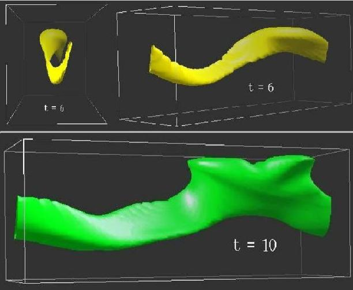
Figure 3.: Three-dimensional visualization of a rising flux tube in the presence of rotation. The stratification is adiabatic such that temperature, pressure, and density all vanish at a height that is about 30% above the vertical extent shown. (The actual computational domain was actually larger in the $x$ and $z$ directions.)

In future simulations we plan to follow the emergence of the flux tube into the outer low plasma-beta exterior. We expect that the losses of magnetic helicity have a scale dependence that follows roughly that in the exterior. In the following subsection we discuss the consequences of surface losses of helical magnetic fields at small and large scales.

4. Phenomenology of small and large scale field losses

A relatively useful concept is based on the evolution equations for small and large scale fields under the assumption that the fields are maximally helical and have opposite signs of magnetic helicity at small and large scales. The details can be found in Brandenburg, Dobler, & Subramanian (2002, Sect. 4.2). The strength of this approach is that it is quite independent of mean-field theory.

Losses of large-scale field have been modeled using diffusion terms. The phenomenological evolution equation are written in terms of the magnetic energies and large and small scales, $M_{\rm m}$ and $M_{\rm f}$, respectively, where we assume $M_{\rm m}=\pm\mu_{0}C_{\rm m}/k_{\rm m}$ and $M_{\rm f}=\mp\mu_{0}C_{\rm f}/k_{\rm f}$ for fully helical fields (upper/lower signs apply to northern/southern hemispheres). The phenomenological evolution equation take then the form

$${{\rm d}M_{\rm m}\over{\rm d}t}=-2\eta_{\rm m}k_{\rm m}M_{\rm m}+2\eta_{\rm f}k_{\rm f}M_{\rm f},$$ (6)

where $\eta_{\rm m}$ and $\eta_{\rm f}$ are effective magnetic diffusivities that are expected to be anywhere between the molecular magnetic diffusivity, $\eta$, and the turbulent magnetic diffusivity, $\eta_{\rm t}$. The opposite signs with which $M_{\rm m}$ and $M_{\rm f}$ enter reflect the fact that large and small scales contribute with opposite signs. The case $\eta_{\rm m}=\eta_{\rm f}=\eta$ was already discussed by Brandenburg (2001) who assumed that after a certain time $t_{\rm sat}$, the small scale magnetic field will have saturated, so $M_{\rm f}\approx\mbox{const}$ after $t>t_{\rm sat}$. After that time, Eq. (6) can be solved and yields the solution

$$M_{\rm m}={\eta_{\rm f}k_{\rm f}\over\eta_{\rm m}k_{\rm m}}\left[1-e^{-2\eta_{\rm m}k_{\rm m}^{2}(t-t_{\rm sat})}\right],\quad\mbox{for $t>t_{\rm sat}$}.$$ (7)

This equation shows three things:

• The time scale on which the large scale magnetic energy evolves depends only on $\eta_{\rm m}$, not on $\eta_{\rm f}$.

• The saturation amplitude diminishes as $\eta_{\rm m}$ is increased, which compensates the accelerated growth just past $t_{\rm sat}$ (Brandenburg & Dobler 2001).

• The reduction of the saturation amplitude due to $\eta_{\rm m}$ can be offset by having $\eta_{\rm m}\approx\eta_{\rm f}$, i.e. by having losses of small and large scale fields that are about equally important.

The overall conclusion that emerges from this is, (i) $\eta_{\rm m}>\eta$ in order that the large scale field can evolve on a time scale other than the resistive one, and (ii) $\eta_{\rm m}\approx\eta_{\rm f}$ in order that the saturation amplitude is not catastrophically diminished. These requirements are perfectly reasonable, but so far they have not been borne out by simulations. Brandenburg & Dobler (2001) found that most of the losses of magnetic helicity occur on large scale. This is at first glance very surprising, but on the other hand the magnetic helicity is a quantity that is strongly dominated by the large scales. However, certain phenomena such as CMEs and other perhaps less violent surface events are not presently included in the simulations. As a proof of concept, however, it has been possible to show that the artificial removal of small scale magnetic fields (via Fourier filtering after a certain number of time steps) can indeed lead to significant increase of the saturation amplitude.

The role of boundaries becomes particularly evident when considering the fact that for closed or periodic boundaries the net flux through a surface bounded by such boundaries cannot change. Indeed, the large scale fields considered in Brandenburg (2001) also satisfy this property, so the mean field is not simply the field averaged over the entire box, but just horizontal averages.

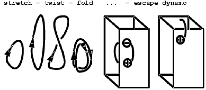
Figure 4.: Stretch-twist-fold (STF) dynamo with subsequent flux loss through the upper boundary, leading to the production of net flux through the box. (Adapted from Brandenburg 1998)

The standard picture of a generic dynamo is the stretch-twist-fold (STF) dynamo, which is depicted in Fig. 4. The flux through one half of the loop has doubled after one STF iteration which, after gluing the two overlying loops together, has lead to a configuration that is topologically equivalent to the initial one. There is one slight subtlety however: (a) after having twisted and folded the two parts of the loop together we have simultaneously introduced internal twist into the tube, very much like the internal twist seen in Fig. 1. Again, this happened only because magnetic helicity is such a well conserved quantity, while still small and large scale magnetic helicity have been introduced simultaneously.

As this twisted configuration goes through the boundary, magnetic flux is lost partially, leaving a finite net magnetic flux through the cross-section of the entire interior domain (see the second part of Fig. 4). At the same time, though, no net magnetic helicity is lost because the loop simultaneously contains two canceling contributions. That such a loop has zero net helicity may be difficult to observe in practice because the twist along the tube, which corresponds to the small scale contribution, may be unresolvable if the overall structure is too small. Another perhaps more plausible proposition is that the magnetic helicity observed so far does already come from the small scales, and that it is the large scale contribution that is not yet observed.

5. Conclusions

In this paper we have emphasized the importance of trying to detect simultaneously large and small scale contributions to the losses of helical magnetic fields at the solar surface. The motivation comes mostly from isotropic turbulence simulations (similar high resolution simulations of more realistic settings do not seem to be available yet), but the basic reasoning is sufficiently general to warrant tentative application to the sun. If our picture is correct, it would predict the existence of an as yet unidentified helical component of the magnetic field (with positive magnetic helicity in the northern hemisphere). We expect that this unidentified component should be associated with the large scale field rather than the small scale field. The reason such a component is difficult to detect is related to the fact that the large scale field is not seen directly. It only manifests itself through the systematic orientation of bipolar regions. However, such indirect indications have also been used in the past to estimate the temporal–latitudinal behavior of the large scale magnetic field from synoptic charts (Yoshimura 1976, Stix 1976). This approach should be repeated with more complete recent data to assess at least the sign of the large scale magnetic helicity.

Acknowledgments.

Use of supercomputer time on the PPARC supported machines at Leicester and St Andrews, as well as the 512 node Beowulf cluster in Odense is acknowledged.

References

Abbett, W. P., Fisher, G. H., & Fan, Y. 2000, ApJ, 540, 548

Bao, S. D., Zhang, H. Q., Ai, G. X., & Zhang, M. 1999, A&AS, 139, 311

Berger, M., & Field, G. B. 1984, JFM, 147, 133

Berger, M. A., & Ruzmaikin, A. 2000, JGR, 105, 10481

Blackman, E. G. & Field, G. B. 2000, MNRAS, 318, 724

Brandenburg, A. 1998, in Theory of Black Hole Accretion Discs, ed. M. A. Abramowicz, G. Björnsson & J. E. Pringle (Cambridge University Press), 61

Brandenburg, A. 2001, ApJ, 550, 824

Brandenburg, A. 2002, in Simulations of magnetohydrodynamic turbulence in astrophysics, ed. T. Passot & E. Falgarone (Springer Lecture Notes in Physics), (in press) (astro-ph/0207394)

Brandenburg, A., & Dobler, W. 2001, A&A, 369, 329

Brandenburg, A., Bigazzi, A., & Subramanian, K. 2001, MNRAS, 325, 685

Brandenburg, A., Dobler, W., & Subramanian, K. 2002, AN, 323, 99 (astro-ph/0111567)

Chae, J. 2000, ApJ, 540, L115

Choudhuri, A. R., Schüssler, M., & Dikpati, M. 1995, A&A, 303, L29

Démoulin, P., Mandrini, C. H., van Driel-Gesztelyi, L., Lopez Fuentes, M. C., & Aulanier, G. 2002, Solar Phys., 207, 87

DeVore, C. R. 2000, ApJ, 539, 944

Durney, B. R. 1995, Solar Phys., 166, 231

Ji, H. 1999, PRL, 83, 3198

Krause, F., & Rädler, K.-H. 1980, Mean-Field Magnetohydrodynamics and Dynamo Theory (Akademie-Verlag, Berlin; also Pergamon Press, Oxford)

Küker, M., Rüdiger, G., & Schultz, M. 2001, A&A, 374, 301

Longcope, D. W., & Klapper, I. 1997, ApJ, 488, 443

Low, B. C. 2001, JGR, 106, 25,141

Moffatt, H. K. 1978, Magnetic Field Generation in Electrically Conducting Fluids (Cambridge University Press, Cambridge)

Parker, E. N. 1955, ApJ, 122, 293

Parker, E. N. 1979, Cosmical Magnetic Fields (Clarendon Press, Oxford)

Pevtsov, A. A. & Latushko, S. M. 2000, ApJ, 528, 999

Pevtsov, A. A., Canfield, R. C., & Metcalf, T. R. 1995, ApJ, 440, L109

Pouquet, A., Frisch, U., & Léorat, J. 1976, JFM, 77, 321

Rust, D. M. & Kumar, A. 1996, ApJ, 464, L199

Rädler, K.-H., & Seehafer, N. 1990, in Topological Fluid Mechanics, ed. H. K. Moffatt & A. Tsinober (Cambridge University Press, Cambridge), 157

Seehafer, N. 1990, Solar Phys., 125, 219

Seehafer, N. 1996, Phys. Rev., E 53, 1283

Stix, M. 1976, A&A, 47, 243

Zeldovich, Ya. B., Ruzmaikin, A. A., Sokoloff, D. D. 1983, Magnetic fields in astrophysics (Gordon & Breach, New York)

Yoshimura, H. 1976, Solar Phys., 50, 3