The Enigmatic HH 255

Abstract

To gain insight into the nature of the peculiar Herbig-Haro object HH 255 (also called Burnham’s nebula), we use previously published observations to derive information about the emission line fluxes as a function of position within HH 255 and compare them with the well-studied, and relatively well-behaved bow shock HH 1. There are some qualitative similarities in the H$\alpha$ and [O III] 5007 lines in both objects. However, in contrast to the expectation of the standard bow shock model, the fluxes of the [O I] 6300, [S II] 6731, and [N II] 6583 lines are essentially constant along the axis of the flow, while the electron density decreases, over a large distance within HH 255.

We also explore the possibility that HH 255 represents the emission behind a standing or quasi-stationary shock. The shock faces upwind, and we suggest, using theoretical arguments, that it may be associated with the collimation of the southern outflow from T Tauri. Using a simplified magnetohydrodynamic simulation to illustrate the basic concept, we demonstrate that the existence of such a shock at the north edge of HH 255 could indeed explain its unusual kinematic and ionization properties. Whether or not such a shock can explain the detailed emission line stratification remains an open question.

1 Introduction

Outflows from young stellar objects (YSO’s) are complex and dynamic, always resulting in violent interactions with circumstellar material and internal interactions within the flow. The most conspicuous optical manifestation of these hypersonic interactions are Herbig-Haro (HH) objects, which cool primarily by emission from hydrogen recombination and collisionally excited, forbidden emission lines from metals. Undeniably, the study of these outflows is an important part of understanding the star formation process as a whole (for a review, see Reipurth & Bally, 2001).

Burnham’s nebula, called HH 255 by Reipurth (1999) and condensation E by Böhm & Solf (1994, hereafter BS94), is part of the circumstellar material south of T Tauri and seems to be a part of the complex HH outflow from that star forming region. A number of studies have demonstrated that the forbidden line fluxes in HH 255 agree quite well with the characteristic shock-excited spectrum of an HH object (Herbig, 1950, 1951; Schwartz, 1974; Solf, Böhm, & Raga, 1988, hereafter SBR88). However, the spatially resolved and detailed spectra of HH 255 reveal some properties that are difficult to understand, in the context of a typical HH bow shock (BS94; Böhm & Solf, 1997; Solf & Böhm, 1999, hereafter BS97 and SB99).

The first obvious problem is that, while the high ionization lines of [O III] and [S III] in HH 255 are quite similar to those of HH 1 (a representative HH object) and require a shock velocity of $>90$ km s^-1, the measured radial velocity of HH 255 is very nearly zero, with respect to the photospheric velocity of T Tau (SBR88; BS94). One may try to explain this problem by arguing that HH 255 is seen nearly side on or that it is a stationary feature, such as a shocked ambient cloudlet. However, SBR88 and SB99 find an inclination of the blue-shifted, southern T Tau outflow of $\sim 14^{\circ}$ and $11^{\circ}$ (respectively) from the plane of the sky, too large to account for the small radial velocity. The shocked cloudlet explanation (which implies the existence of a bow shock facing toward T Tau) is ruled out by the velocity dispersion observed in HH 255. That is, the total velocity dispersion (full width at zero intensity) of optical forbidden lines in HH 255 is unusually small, less than 45 km s^-1 (BS97). It is well known that bow shocks exhibit a large velocity dispersion, comparable to (and most often greater than) the shock velocity (see Hartigan, Raymond, & Hartmann, 1987; Raga & Böhm, 1986; Choe, Böhm, & Solf, 1985), as material that enters the front of the shock is then accelerated roughly perpendicular to the original flow direction and eventually moves around the obstacle (e.g., the bullet, jet, or cloudlet). In addition, the velocity dispersion of the forbidden ionic and atomic lines in HH 255 is the same as for molecular H₂ lines (SB99). This is surprising, since the H₂ lines form at much lower shock velocity, and therefore typically come from a region with a smaller velocity dispersion than the optical lines in HH objects. Another partial explanation would be that HH 255 results from a plane shock. This could explain the low centroid velocity and velocity dispersion, but BS97 pointed out that the cooling region would have a thickness of only about 0$\farcs$1, while HH 255 shows nearly constant ionization from about 4″–10″ south of T Tau. Also, the possible existence of a plane shock in an HH flow lacks a theoretical explanation.

The enigmatic ionization structure and kinematic properties of HH 255 prompt us to look in more detail at data obtained earlier from SBR88, BS94, BS97, and SB99. We do this to gain a more complete picture of all observable properties to guide the models of this object. In addition, we further explore the possibility that HH 255 is a stationary shock (that is neither a plane shock nor a bow shock). First we review the known properties of HH 255 in section 2. In section 3, we look at the emission line fluxes as a function of position along HH 255 and compare them to those of HH 1. Finally, section 4 discusses the interpretation of HH 255 as a standing shock, possibly associated with the collimation of the outflow south of T Tauri.

2 Known Properties of HH 255

T Tauri is a binary system (Dyck, Simon, & Zuckerman, 1982) at a distance of about 140 parsecs (see, e.g., Reipurth, Bally, & Devine, 1997). It consists of a visible stellar component, T Tau N, and an infrared source T Tau S (discovered by Dyck et al., 1982), located about 0$\farcs$62 south of T Tau N. Robberto et al. (1995) presented coronagraphic mages of the complex emitting environment around T Tau. Spectroscopically, SB99 identified two separate outflows moving almost perpendicular to each other, consisting of an E–W outflow (e.g., HH 155, discovered by Schwartz, 1975) originating from T Tau N and a N–S outflow originating from the embedded source, T Tau S. Reipurth et al. (1997) proposed that the N–S outflow is the likely source for the giant outflow HH 355.

In their high spatial and spectral resolution spectroscopic study of the T Tau environment, BS94 identified several kinematic components (A, B, C, D, and E) of the outflows. Component E coincides with HH 255 and lies south of T Tau, along the N–S outflow. The components of the N-S outflow near T Tau are apparent in Figure 1, a position-velocity diagram from the [S II] 6731 line at a position angle of $0^{\circ}$/$180^{\circ}$. SB99 carried out a deeper spectroscopic study and identified two more components, I and J, of the N–S outflow. Component I lies about 10″ north and J lies about 15″ south of T Tau. By considering only the components C, D, I, and J, SB99 derived an inclination of $\sim 11^{\circ}$ from the plane of the sky for the N–S outflow. This inclination implies a total outflow velocity of $\sim 90$ km s^-1 for I and J and $\sim 280$ km s^-1 for C and D.

HH 255 (component E) lies along the outflow south of T Tau, but it possesses unusual kinematic behavior (as noted in §1 and described below). There are two possibilities: Either HH 255 is physically associated with the T Tau outflow, or it is simply projected onto the region between condensations D and J and coincidently has the same radial velocity as T Tau. In the unlikely event that it is a projected object, HH 255 remains mysterious (i.e., it still exhibits an HH spectrum with unusual kinematic behavior). In addition, the position-velocity diagram (Fig. 1) contains possible evidence for a physical connection with component D. First, HH 255 seems to begin at the same place where D disappears (D extends to about 4″, while E spans from roughly 4″ to 10″ south of T Tau). Also, BS94 note an apparent “bridge” of emission between D and E in the position-velocity diagram (most evident in [N II]), suggesting a rapid decline in radial velocity at the edge of component D that “connects” to the low radial velocity of HH 255. Therefore, we will hereafter assume that HH 255 is physically associated with the outflow south of T Tau.

The spectrum of HH 255 is consistent with a moderately high excitation HH object (SB88; Raga, Böhm, & Cantó, 1996), suggesting that it is emission from shock-excited gas. Further evidence for a shock was found by BS97, who derived information about the ionization, centroid velocity, and velocity dispersion from emission lines in components D and E. They found an essentially discontinuous rise (as one moves south) of the line ratios [O III]/H$\alpha$, [N II]/[N I], and [O II]/[O I] between a distance of 3″ and 4″ south of T Tau, indicating a drastic increase in ionization there. Beyond that, the ionization is roughly constant from 4$\farcs$5 to 8$\farcs$5. The centroid velocity (of, e.g., [N II]) has maximum (blueshift) of roughly $-45$ km s^-1 at 2″ (inside component D), decreases to $-25$ km s^-1 from 2$\farcs$5 to 3$\farcs$5, and then plummets to basically zero from 3$\farcs$5 to 4$\farcs$5. The centroid velocity remains near zero (ranging from $0$ to $-5$ km s^-1) from 4$\farcs$5 to about 10″ (within HH 255). The decreasing centroid velocity and increasing ionization (as one moves from D to E) suggests the existence of a shock that faces toward T Tau. That is, material is rapidly decelerated at a position of $\sim 4\arcsec$, and the kinetic energy of the flowing material is converted into thermal energy via a shock.

The presence of [O III] in the spectrum of HH 255 requires a shock velocity (i.e., pre-shock velocity minus post-shock velocity) of $>90$ km s^-1 (Hartigan et al., 1987). The difference in the deprojected velocities of component D and HH 255 allow for such a shock velocity. However, the shock model becomes complicated when one considers the behavior of the velocity dispersion in the shocked region. BS97 found that velocity dispersion (the full width at half maximum of [N II] and [S II]) falls from about 80 km s^-1 at 3$\farcs$5 to about 25 km s^-1 at 4$\farcs$5 and remains the same to about 9″ south of T Tau. Bow shock models (e.g., Hartigan et al., 1987; Raga & Böhm, 1985, 1986) predict that the velocity dispersion should increase where the centroid velocity decreases. In contrast, at the interface between component D and E, both the centroid velocity and the velocity dispersion decrease at the same location. Further, the bow shock models predict that the full width at zero intensity (FWZI) of observed lines should be equal to the shock velocity (Hartigan et al., 1987; Raga & Böhm, 1985, 1986). In HH 255, the FWZI (as estimated by the full width at 10% intensity) remains constant at about 45 km s^-1 (BS97), well below the minimum shock velocity of $90$ km s^-1 required by the [O III] flux.

This means that HH 255 is not a bow shock. Unlike typical HH objects (Hartigan et al., 2000; Raga et al., 1996), it is not a working surface within or at the head of a jet or bullet, and it cannot be a shock around a stationary cloudlet. On the other hand, the fact that the centroid velocity is almost zero and the velocity dispersion is very small suggests that HH 255 is a standing shock with some shape other than a bow. We will discuss this possibility further in section 4. It is clear that, in order to understand HH 255, we have to study additional observational properties of this emission region. So far, most of its enigmatic properties have been deduced from the kinematics and ionization, so in the next section, we use existing data to derive information about the line flux and density within HH 255.

3 Line Flux and Density Stratification

In order to gain more insight, we will look at the emission line fluxes as a function of position along HH 255 derived from previous observations. We focus specifically on the well-observed lines H$\alpha$, [O I] 6300, [S II] 6731, [N II] 6583, and [O III] 5007. We know that components D and J are parts of the southern outflow, which moves nearly perpendicular to the line of sight (SB99), and we will assume that HH 255 (component E) is a part of that outflow. We shall also make use of the fact that HH 1 is a well-studied and relatively well-behaved bow shock (SBR88; Choe et al., 1985; Hartigan et al., 1987; Solf & Böhm, 1991; Reipurth & Bally, 2001; Bally et al., 2002). Since HH 255 and HH 1 have the same overall excitation, and both are seen nearly side-on, one would naively expect that the line flux stratification of each line would be similar for both objects. Therefore, in the following study, we will compare HH 255 to HH 1. One must be aware that typical HH objects conform to a simple bow shock model only very approximately, at best, so we do not expect more than a crude, qualitative agreement between the two objects. Also, the enigmatic ionization structure and kinematic properties of HH 255 (discussed in §2) already show that it is unique.

The observational data that we need for this investigation can be extracted from the earlier studies of SBR88, BS94, BS97, and SB99. For instance, SBR88 present information about the ratios [O I]/H$\alpha$, [S II]/H$\alpha$, [N II]/H$\alpha$, and [O III]/H$\alpha$, and about H$\alpha$ itself, along a line from 2$\farcs$7 to 10$\farcs$0 south of T Tau. Additional information about some of the lines (with higher spatial and spectral resolution) has been extracted from BS94. Information about line emission at larger distance from T Tau (which we used only indirectly) is available in SB99.

In Figure 2, we show the H$\alpha$ and [O III] line fluxes as a function of position south of T Tau. We focus on the region containing the transition between component D and HH 255 (from $\sim 3\arcsec$–4$\farcs$5) and also following the entire extent of HH 255. The fluxes of each line are given in arbitrary units (note that line ratios derived from this plot would not be correct). It is evident in Figure 2 that [O III] peaks in the transition region and decreases (though gradually) with distance inside HH 255. Component D (which is an important part of the N–S outflow; see §2) does not contribute significantly to the [O III] emission. On the other hand, the H$\alpha$ line is relatively bright in component D, which is fairly close to T Tau, and decreases rapidly to the northern edge of HH 255. Within HH 255, H$\alpha$ also decreases gradually with distance from T Tau before decreasing rapidly again at the southern edge of HH 255.

For comparison, we plot the H$\alpha$ and [O III] line fluxes in HH 1 along the extrapolated jet axis in Figure 3. Since the HH 1 bow shock points away from the outflow source (in contrast to HH 255, see §2), we have plotted the distance in arcseconds, from an arbitrary starting point, moving toward the source (i.e., in the opposite sense as in Fig. 2). We have chosen this orientation so that pre-shock material is plotted on the left hand side of both Figures 2 and 3, and post-shock material is on the right. There are two things to consider when comparing the apparent length scales in these two Figures. First, HH 1 is about three times further away than T Tauri. Second, the characteristic length scales (e.g., the cooling length) of each object will be different because of the different pre-shock particle densities and the different sizes and shapes of the jets that drive each shock. The two effects partially cancel to give an apparent spatial size of HH 1 that is roughly similar to HH 255.

A comparison between Figures 2 and 3 reveals a qualitative agreement in [O III]. Both objects exhibit a rise in [O III] and a subsequent decline. The decline of [O III] in HH 255, however, is apparently slower than in HH 1. The H$\alpha$ emission in HH 1 behaves the same as [O III]. This is not the case for HH 255. The steep decline of H$\alpha$ to the northern edge of HH 255 is typical of many T Tauri stars and probably has nothing to do with the transition region between component D and HH 255. The decline of H$\alpha$ within HH 255 is similar to the decline of H$\alpha$ in HH 1. However, the decline is apparently slower in HH 255, and beyond 8$\farcs$5, the H$\alpha$ emission drops off suddenly much more steeply. The increase in [O III] and gradual decline of [O III] and H$\alpha$ (present in both objects) conforms to the general model of a cooling/recombination region behind a shock. This rough agreement between Figures 2 and 3 strengthens the assumption that HH 255 arises from emission behind a shock that faces toward the outflow source, while the HH 1 bow shock points away from its source.

Figures 4 and 5 contain the flux distribution for HH 255 and HH 1 (respectively) of the [O I], [S II], and [N II] lines. In these lines, the fluxes along HH 255 (Fig. 4) are drastically, though systematically, different from the results in HH 1 (Fig. 5). The behavior of [O I], [S II], and [N II] in HH 1 (Fig. 5) is basically the same as for [O III] and H$\alpha$ (discussed above; Fig. 3) and represents the expected behavior for a bow shock. By contrast, the emission lines in Figure 4 remain surprisingly constant (to within 10% for [N II], 18% for [S II], and 9% for [O I]) along the extent of HH 255, between 4″ and 9″ south of T Tau (corresponding to a distance of $\sim 700$ AU). Beyond this point, the fluxes decrease steeply. The steep decrease occurs in the same place for all three lines (and for H$\alpha$ in Fig. 2), so it cannot be a consequence of a change in ionization. This could be the consequence of a drastic increase in the line of sight extinction at that location, but the most likely explanation is a rapid decline in the general particle density at about 9″ south of T Tau. As far as we know, this behavior has not been seen before in any part of an outflow from a T Tauri star.

The unusual fact that the emission line fluxes of [O I], [S II], and [N II] remain constant throughout HH 255 should be discussed further. Remember that these forbidden emission lines are generated by radiative de-excitation to the ground state by atoms that have been excited by collisions with free electrons (see, e.g., Osterbrock, 1989). In this context, the electron density, $N_{\rm e}$, is an important quantity, so we have plotted $N_{\rm e}$ as a function of position south of T Tau in Figure 6. The two lines in the Figure represent data from two studies (SBR88; BS94), and they are in agreement with each other (though the measurements were taken at different epochs). Note that the electron density in HH 255 is relatively low (always $<3\times 10^{3}$ cm^-3), so collisional de-excitation is not an important process. Since the ionization state of the gas is roughly constant within HH 255 (BS97), a simple explanation for the constancy of emission lines would be that $N_{\rm e}$ and the particle density are also constant throughout. It is clear from Figure 6, however, that this explanation is not acceptable because $N_{\rm e}$ decreases by a factor of two or three along HH 255.

The volume emissivity (emission per cm³) for a given line of a given species is proportional to $N_{\rm e}N_{\rm s}$, where $N_{\rm s}$ is the number density of the species. The measured fluxes shown in Figure 4 represent the emission per cm² (since all of the emission adds along the line of sight). The fact that $N_{\rm e}$ decreases, while the line fluxes are constant, requires a strict relationship between the geometry, velocity, and/or time-dependence of the outflow within HH 255. In the next section, we will discuss a plausible model for the flow that explains some (but not all) of the observations.

4 Discussion

4.1 Summary of Properties

We have presented convincing evidence that the northern edge of HH 255 is a reverse-facing shock in the southern outflow of T Tau. The kinematic structure of the shock (see §2) is drastically different than expected for a bow shock, which is the successful model for typical HH objects. The emission region behind the shock, which comprises the extent of HH 255 itself, is also unusual, requiring a flow structure in which the electron density decreases, while some of the line fluxes remain constant over a large fraction of the flow (see §3). Some of the basic properties of HH 255 can be summarized as follows:

1. The ionization state is consistent with emission excited by a shock, and the strength of [O III] 5007 emission requires a shock velocity of greater than 90 km s^-1. The ionization is roughly constant along the extent of HH 255.

2. The radial velocity, $v$, goes nearly to zero across the shock, at the same place where the velocity dispersion, $\Delta v$, decreases. Behind the shock, $\Delta v$ remains less than 45 km s^-1 along the extent of HH 255. In contrast, bow shock models predict that the $\Delta v$ increases where the $v$ decreases, and that $\Delta v$ is equal to the shock velocity.

3. The electron density, $N_{\rm e}$, has a maximum at the location of the shock, then decreases by a factor of 2–3 along the extent of HH 255 (see Fig. 6).

4. The fluxes of the [O I] 6300, [S II] 6731, and [N II] 6583 lines are constant along the extent of HH 255.

5. At the southern edge of HH 255, the fluxes of the [O I], [S II], [N II], and H$\alpha$ lines decrease drastically and simultaneously.

4.2 A Preliminary Model

We would like to find a model that, at least partially, explains the enigmatic properties of HH 255 listed above. To that end, we propose that HH 255 results from a standing or quasi-stationary shock, possibly associated with the collimation of the southern outflow (or part of that flow) from T Tau. A basic introduction of standing shocks, and the distinction between a receding and a stationary shock, was originally given by Courant & Friedrichs (1948).

There is a theoretical justification for expecting reverse-facing, slow-moving shocks near the collimation region of outflows from YSO’s. Models for the launching of such outflows (for a review, see Shibata & Kudoh, 1999; Königl & Pudritz, 2000) rely on magnetic processes within the wind that lead to a self-collimation of material near the axis into a jet. However, not all of the material in the launched wind is collimated, so the models predict outflows with both a collimated and a wide-angle component (e.g., Li & Shu, 1996). Observational support for a two component wind very near the central star (i.e., a jet plus a wide-angle “disk wind”) was noted by Kwan & Tademaru (1988). Recently, a few authors (Frank & Noriega-Crespo, 1994; Frank & Mellema, 1996; Mellema & Frank, 1997; Delamarter, Frank, & Hartmann, 2000; Gardiner, Frank, & Hartmann, 2002; Matt, 2002; Matt, Winglee, & Böhm, 2003) have shown that the interaction between the wide-angle wind and the circumstellar environment results in a reverse-facing shock that is stationary or moves slowly with respect to the head of the collimated jet (see also Frank, Gardiner, & Lery, 2002). The reverse shock completely encloses the wind and bears no morphological or kinematic resemblance to a bow shock. These authors have also shown that, depending on the details of the wind and its environment, the wide-angle wind can itself become collimated by thermal or magnetic pressure gradients in the post-shock region, adding to the total collimated flow and leading to broader and more powerful jets than in the pre-shock, free-flowing wind.

It is not clear what the observational signature of this reverse-shock would be. To our knowledge, no one has claimed to observe such a feature in a YSO outflow (though such a possibility is discussed in the very recent work of Bally, Feigelson, & Reipurth, 2002). Presumably, the reverse shock exists relatively close to the source (within a distance that is comparable to the width of the collimated outflow) and would therefore be difficult to disentangle from the complex emitting environment there.

To get more insight into this problem, and to serve as an illustrative example, we have run a very simplified numerical magnetohydrodynamic (MHD) simulation of the interaction between an isotropic central wind and a constant, vertical magnetic field held fixed on a plane (as if fixed in a disk). This work is similar to that of Matt (2002), and we have used their 2.5D (axisymmetric) MHD simulation code (the code is also described in Matt et al., 2002). The code uses a two-step Lax-Wendroff (finite-difference) scheme to solve the equations on a group of nested, Eulerian grids. For this very simple, illustrative case, we consider only the effects of ideal MHD on an adiabatic plasma, and we ignore the effects of gravity and rotation.

For the central wind boundary condition, we use a sphere with a radius of 40 grid points, corresponding to 40 AU. There, the wind turns on at $t=0$ and is held constant and radial with a velocity of 280 km s^-1 (with a Mach number of 5) and a mass outflow rate of $2\times 10^{-8}M_{\odot}$ yr^-1 (consistent with the known properties of the southern T Tau outflow and with typical HH outflows; Reipurth & Bally, 2001). The rest of the grid is initialized with a constant density of 60 particles per cm³ and a constant magnetic field of $10^{-3}$ Gauss (the ratio of the Alfvén to sound speed in the ambient environment is 5). At the cylindrical $z=0$ boundary, we held the magnetic flux constant and did not allow outflow or inflow onto the boundary. In this way, the magnetic field lines are “anchored” at the equator as if embedded in a geometrically thin, conducting disk. We use outflow boundary conditions on the outer boundaries of our outermost grid (of which there were 5, nested concentrically).

When the simulation begins, the wind propagates outward, and sweeps up the ambient material and vertical magnetic field ahead of it. With the chosen parameters, the kinetic energy in the wind (which goes roughly as $r^{-2}$) becomes equal to the ambient magnetic energy density (which is constant for a vertical field) at a radius of about 500 AU. At this location, there is a reverse-facing shock where the wind converts some of its kinetic energy to thermal energy. This shock is stagnant, and the steady-state solution contains a jet composed of post-shock wind gas. Figure 7 shows the density (logarithmic), velocity vectors, and magnetic field lines of this steady-state solution achieved in the simulation.

The Figure is not intended to represent the southern outflow of T Tau in any detail, but it illustrates some of the key features of our proposed explanation. Most importantly, there is a reverse-facing shock that is stagnant at a position of about 500 AU (corresponding to 3″-4″ at the distance to T Tau) along the $z$ direction in Figure 7. The shock does not resemble a bow shock morphologically nor kinematically, as post-shock material does not have a large velocity dispersion as it moves essentially vertically within the jet. Since the magnetic field is fixed on the equator (in this particular example), the flow at wide angles hits an oblique shock, which compresses and forms a sort of shell of relatively fast moving material around the flow that continues past 500 AU. This feature is dependent on the details of this type of collimator, and we do not mean to suggest that such a feature exists in HH 255. In the next section, we will compare the expected behavior of the proposed stationary shock to the observed properties of HH 255.

4.3 Comparison of Model to HH 255

Figure 1 shows that, at $\sim 4$″ south of T Tau, there is an abrupt transition in velocity. It starts from a centroid radial velocity of $-45$ km s^-1 in component D (which corresponds to a total velocity of $-280$ km s^-1; see §2 and SB99), and decreases to only a few km s^-1 in HH 255 (also see fig. 5 of BS97). The velocity dispersion decreases in the same region. Furthermore, the ionization of N and O increases drastically southward between 3″ and 4″ south of T Tau, and the electron density has a maximum in the same region (BS97).

These properties at the northern edge of HH 255 would be rather well explained by the existence of a standing shock. In any sort of ionizing shock, the velocity will decrease at the same place that the density and ionization state increases. However, the velocity dispersion will only be low (as in HH 255) if post-shock gas flows through the shocked region and does not diverge rapidly (i.e., to move around some obstacle; as in the case of a bow shock).

To illustrate this point further, and for comparison to Figure 1, we generated an artificial position-velocity diagram (Fig. 8) from the simulation data in our illustrative example discussed in section 4.2. To do this, we used our steady-state solution plotted in Figure 7. With the assumption of axisymmetry, we generated a 3D data cube, placed the observer along the cylindrical $r$ direction (i.e., the observer sees the jet in the plane of the sky), and made a histogram of velocities as a function of $z$. Because we are interested in where the most emission is likely to occur, we weighted the velocities in the histogram by the density squared. Furthermore, we only considered the material within a slit aperture with a width of 140 AU (corresponding to the 1″ slit width used by BS94). The data has been smoothed to a spatial resolution of roughly 30 AU and we used a velocity binning corresponding to a resolution of about 15 km s^-1. Figure 8 contains the resulting position-velocity diagram. Note that the vertical distance scale is reversed, with respect to Figure 7.

It is clear from Figure 8 that, at the location of the reverse shock ($\sim 500$ AU), the velocity dispersion becomes quite small compared to the shock velocity of nearly 280 km s^-1. Figures 1 and 8 do not agree at all in the region closer to the star than 500 AU. Note that, in Figure 1, the region near the star is dominated by the emission from component D and emission from other parts of both outflows (N–S and E–W) from T Tau. In Figure 8, the structure in region near the star depends on the details of the specific example we chose, and the very broad width (e.g., compared to component D in Fig. 1) is due to the fact that the simulated central wind is completely isotropic (a partially collimated central wind could have a much narrower $\Delta v$). In spite of this, the region from 500 AU and beyond in Figure 8 is qualitatively quite similar to component E (HH 255) in Figure 1. This general similarity demonstrates that a reverse-facing, stationary shock at the position of 500 AU may explain some of the unusual spatio-kinematic properties of HH 255.

There are other aspects of the observations, however, that are more difficult to explain, without considering the radiative properties of the shock. Specifically, the details of the emission distributions of the H$\alpha$, [O III], [N II], [S II], and [O I] emission lines throughout HH 255 (discussed in §3) have not been explained. It is not obvious that a standing shock, as discussed in section 4.2, should lead to a fundamentally different line emission distribution than a bow shock. In fact, we did find in section 3 that, in HH 255, the [O III] and H$\alpha$ emission agrees somewhat with the prediction of simplified bow shocks (see also Fig. 9 of Raga & Böhm, 1985). We have also not explained the formation of molecular H₂ lines, which presumably form in low velocity (tens of km s^-1) shocks. However, the existence of a reverse shock does explain how the optical forbidden emission lines can have a $\Delta v$ that is comparable to the typical (for HH objects) $\Delta v$ of H₂ lines, as is the case for HH 255 (SB99).

Perhaps the biggest problem, however, is that the fluxes of the [N II], [S II] and [O I] lines are essentially constant, while the electron density decreases, over a large distance within HH 255 (§3). In the adiabatic simulation shown in Figure 7, the density goes from 40 to 130 cm^-3 (and velocity from 290 to 90 km s^-1) across the shock on axis. The density (and jet width and velocity) remains roughly constant beyond that, so that for a constant temperature, the line fluxes in that region would be constant. But in a true, astrophysical shock at those densities, radiative cooling (and ionization) would play a significant role, leading both to a larger density jump across the shock and to a temperature gradient behind the shock. For example, Shull & McKee (1979) showed that, for a pre-shock density of 10 cm^-3 and a shock velocity of 100 km s^-1, the maximum density behind a radiating shock is 6450 cm^-3, leading to a cooling region that is quite small (of order 10 AU). However, if one ignores the cooling just behind the shock (or if the post-shock density is significantly lower), the cooling time for gas at a density of 10³ cm^-3 is of the order of 100 years (Aller, 1984; Shapiro & Moore, 1976), which is comparable to the crossing time of material in HH 255. At present, we are unable to resolve this dilemma, without doing a detailed and self-consistent cooling (and ionization) calculation for a reverse-facing, standing shock. We leave such a calculation and detailed comparison to the emission line distribution in HH 255 for future work.

At present, it is conceivable that HH 255 is the emission behind a reverse-facing, standing (non bow) shock, possibly associated with the collimation of the southern outflow from T Tau. However, other possibilities have not been fully explored. One potentially important effect is that of time-dependence within the flow that formed HH 255. For example, the fact that the emission of the lines of [N II], [S II], [O I], and H$\alpha$ decrease simultaneously and drastically at the southern edge of HH 255, indicates (most likely) a fast decrease in the matter density. This suggests that, at some earlier time, the flow exhibited an increase in density (or velocity, or both), resulting in the apparent density jump at the southern edge of HH 255. A flow that is not in a steady state (i.e., where the mass continuity equation is not satisfied along the flow) would have spatial distribution of line emission that is different than steady-state models. Also, for simplicity, we have not considered any non-axisymmetric effects.

In some respects, HH 255 has been studied in more detail than any other HH object. Because they noted some peculiar properties, BS94, BS97, and SB99 have studied several physical aspects of HH 255 at high spatial and spectral resolution. It is quite possible that the peculiar behavior of HH 255 is exhibited by other outflows that have escaped being seen (or recognized) in all studies to date. We have shown that HH 255 may have something to do with the interaction of a wide-angle flow with its environment, something predicted (though often indirectly) by essentially all wind launching models. Understanding this interaction may be crucial to our understanding of the collimation of physically broad jets. It would therefore be of great significance if other objects similar to HH 255 are found.

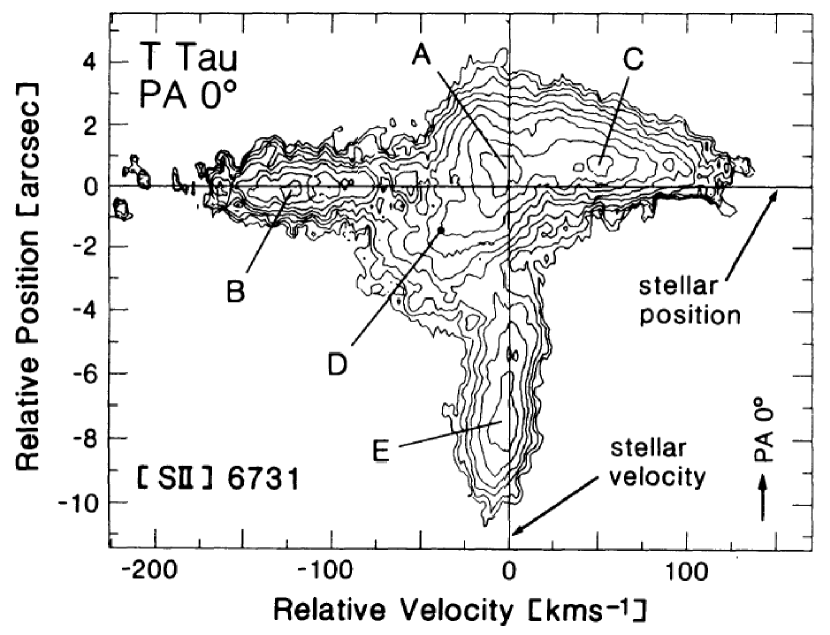
Figure 1: Position-velocity diagram extracted from an echelle observation of the [S II] 6731 line along the position angle of $0^{\circ}$ and centered on T Tauri. This figure was adapted from figures 1b and 2b of Böhm & Solf (1994), who identified the spatio-kinematic components A, B, C, D, and E.

Figure 2: Line fluxes of H$\alpha$ and [O III] 5007 in HH 255 as a function of position south of T Tauri.

Figure 3: Line fluxes of H$\alpha$ and [O III] 5007 in HH 1 as a function of position along the extrapolated jet axis. The distance increases toward the location of the jet source.

Figure 4: Line fluxes of [O I] 6300, [S II] 6731, and [N II] 6583 in HH 255 as a function of position south of T Tauri.

Figure 5: Line fluxes of [O I] 6300, [S II] 6731, and [N II] 6583 in HH 1 as a function of position along the extrapolated jet axis. The distance increases toward the location of the jet source.

Figure 6: Electron density in HH 255 as a function of position south of T Tauri, deduced from the [S II] 6731/6716 line ratio. The squares are from Solf et al. (1988), and the triangles are from Böhm & Solf (1994).

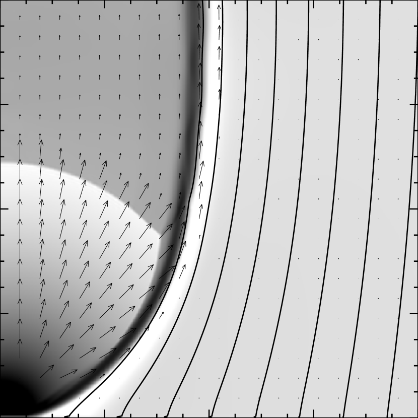
Figure 7: Logarithmic density greyscale (black is highest density, white is lowest), velocity vectors, and magnetic field lines in the steady-state solution of the numerical simulation described in the text.

Figure 8: Artificial position-velocity diagram of the data shown in Figure 7. Shown are logarithmic contours of the velocity histogram as a function of $z$ through a 140 AU wide slit, as seen from a line of sight perpendicular to the jet axis. The stellar position is at the top, and it’s velocity is 0 km s^-1.

References

- Aller (1984) Aller, L. H. 1984, Physics of Thermal Gaseous Nebulae (Dordrecht: Reidel)
- Bally et al. (2002) Bally, J., Feigelson, E., & Reipurth, B. 2002, ApJ preprint doi:10.1086/345850
- Bally et al. (2002) Bally, J., Heathcote, S., Reipurth, B., Morse, J., Hartigan, P., & Schwartz, R. 2002, AJ, 123, 2627
- Böhm & Solf (1994) Böhm, K.-H., & Solf, J. 1994, ApJ, 430, 277 (BS94)
- Böhm & Solf (1997) Böhm, K. H., & Solf, J. 1997, A&A, 318, 565 (BS97)
- Choe et al. (1985) Choe, S.-U., Böhm, K.-H., & Solf, J. 1985, ApJ, 288, 338
- Courant & Friedrichs (1948) Courant, R., & Friedrichs, K. O. 1948, Supersonic Flow and Shock Waves (New York: Interscience)
- Delamarter et al. (2000) Delamarter, G., Frank, A., & Hartmann, L. 2000, ApJ, 530, 923
- Dyck et al. (1982) Dyck, H. M., Simon, T., & Zuckerman, B. 1982, ApJ, 255, L103
- Frank et al. (2002) Frank, A., Gardiner, T. A., & Lery, T. 2002, in Revista Mexicana de Astronomia y Astrofisica Conference Series, ed. W. J. Henney, W. Steffen, A. C. Raga, & L. Binette, Vol. 13, 54
- Frank & Mellema (1996) Frank, A., & Mellema, G. 1996, ApJ, 472, 684
- Frank & Noriega-Crespo (1994) Frank, A., & Noriega-Crespo, A. 1994, A&A, 290, 643
- Gardiner et al. (2002) Gardiner, T. A., Frank, A., & Hartmann, L. 2002, astro-ph/0202243, p. accepted by ApJ
- Hartigan et al. (2000) Hartigan, P., Bally, J., Reipurth, B., & Morse, J. A. 2000, in Protostars and Planets IV, ed. V. Mannings, A. P. Boss, & S. S. Russell (Tucson: Univ. of Arizona Press), 841
- Hartigan et al. (1987) Hartigan, P., Raymond, J., & Hartmann, L. 1987, ApJ, 316, 323
- Herbig (1950) Herbig, G. H. 1950, ApJ, 111, 11
- Herbig (1951) Herbig, G. H. 1951, ApJ, 113, 697
- Königl & Pudritz (2000) Königl, A., & Pudritz, R. E. 2000, in Protostars and Planets IV, ed. V. Mannings, A. P. Boss, & S. S. Russell (Tucson: Univ. of Arizona Press), 759
- Kwan & Tademaru (1988) Kwan, J., & Tademaru, E. 1988, ApJ, 332, L41
- Li & Shu (1996) Li, Z., & Shu, F. H. 1996, ApJ, 468, 261
- Matt et al. (2002) Matt, S., Goodson, A. P., Winglee, R. M., & Böhm, K. 2002, ApJ, 574, 232
- Matt et al. (2003) Matt, S., Winglee, R. M., & Böhm, K.-H. 2003, MNRAS, in preparation
- Matt (2002) Matt, S. P. 2002, Ph.D. Thesis, Astronomy, University of Washington
- Mellema & Frank (1997) Mellema, G., & Frank, A. 1997, MNRAS, 292, 795
- Osterbrock (1989) Osterbrock, D. E. 1989, Astrophysics of Gaseous Nebulae and Active Galactic Nuclei (Mill Valley, CA: University Science books)
- Raga et al. (1996) Raga, A. C., Böhm, K.-H., & Cantó, J. 1996, RMxAA, 32, 161
- Raga & Böhm (1985) Raga, A. C., & Böhm, K.-H. 1985, ApJS, 58, 201
- Raga & Böhm (1986) Raga, A. C., & Böhm, K. H. 1986, ApJ, 308, 829
- Reipurth (1999) Reipurth, B. 1999, A General Catalogue of Herbig-Haro Objects, 2nd ed., http://casa.colorado.edu/hhcat
- Reipurth & Bally (2001) Reipurth, B., & Bally, J. 2001, ARA&A, 39, 403
- Reipurth et al. (1997) Reipurth, B., Bally, J., & Devine, D. 1997, AJ, 114, 2708
- Robberto et al. (1995) Robberto, M., Clampin, M., Ligori, S., Paresce, F., Sacca, V., & Staude, H. J. 1995, A&A, 296, 431
- Schwartz (1974) Schwartz, R. D. 1974, ApJ, 191, 419
- Schwartz (1975) Schwartz, R. D. 1975, ApJ, 195, 631
- Shapiro & Moore (1976) Shapiro, P. R., & Moore, R. T. 1976, ApJ, 207, 460
- Shibata & Kudoh (1999) Shibata, K., & Kudoh, T. 1999, in Star Formation 1999, Proceedings of Star Formation 1999, held in Nagoya, Japan, Nobeyama Radio Observatory, ed. T. Nakamoto, 263
- Shull & McKee (1979) Shull, J. M., & McKee, C. F. 1979, ApJ, 227, 131
- Solf & Böhm (1991) Solf, J., & Böhm, K. H. 1991, ApJ, 375, 618
- Solf & Böhm (1999) Solf, J., & Böhm, K.-H. 1999, ApJ, 523, 709 (SB99)
- Solf et al. (1988) Solf, J., Böhm, K. H., & Raga, A. 1988, ApJ, 334, 229 (SBR88)