NUC-MINN-2002/10-T November 2002 HIGH TEMPERATURE MATTER AND NEUTRINO SPECTRA FROM MICROSCOPIC BLACK HOLES

Abstract

The spectrum of neutrinos produced by the outflow of high temperature matter surrounding microscopic black holes is calculated for neutrino energies between one GeV and the Planck energy. The results may be applicable for the last few hours and minutes of a microscopic black hole’s lifetime.

PACS: 04.70.Dy, 98.70.Sa, 95.85.Ry, 95.55.Vj

1 Introduction

Hawking radiation from black holes [1] is of fundamental interest because it involves the interplay between quantum field theory and the strong field limit of general relativity. It is of astrophysical interest if black holes exist with sufficiently small mass that they explode rather than accrete matter and radiation. Since the Hawking temperature and black hole mass are related by $T_{H}=m_{\rm P}^{2}/8\pi M$, where $m_{\rm P}=G^{-1/2}=1.22\times 10^{19}$ GeV is the Planck mass with natural units $\hbar=c=k_{\rm B}=1$, a present-day black hole will evaporate and eventually explode only if $T_{H}>2.7$ K (microwave background temperature). This requires $M<4.6\times 10^{22}$ kg which is approximately 1% of the mass of the Earth. More massive black holes are cooler and therefore will absorb more matter and radiation than they emit, hence grow with time. Taking into account emission of gravitons, photons, and neutrinos a critical mass black hole today has a Schwarszchild radius of 68 microns and a lifetime of $2\times 10^{43}$ years.

There is uncertainty expressed in the literature about whether the radiation emitted by such small black holes is emitted independently, or whether there is sufficient interaction among the emitted quanta to form a partially thermalized and rapidly expanding fluid around the black hole. Heckler has given arguments in favor of the latter for Hawking temperatures above 1 GeV [2]. Cline, Mostoslavsky and Servant [3] solved the Boltzmann equation in the relaxation-time approximation for such temperatures and found that significant particle scattering did occur, although not enough for perfect fluid flow. One of us showed that a self-consistent description of an outgoing fluid just marginally kept in local equilibrium could be given, but it required the assumption of sufficient initial particle interaction, and viscosity played a crucial role [4]. That paper was followed by an extensive numerical analysis of the relativistic viscous fluid equations by us [5]. We also calculated the spectrum of high energy gamma rays expected during the last days, hours, and minutes of the black hole’s lifetime. We suggested that the most promising route for discovery of such microscopic black holes is to search for point sources emitting gamma rays of ever-increasing energy until suddenly the source shuts off.

In this paper, a follow up to our previous work, we focus on high energy neutrino emission from black holes with Hawking temperatures greater than 100 GeV and corresponding masses less than 10⁸ kg. It is at these and higher temperatures that new physics will arise. Such a study is especially important in the context of high energy neutrino detectors under construction or planned for the future. Previous notable studies in this area have been carried out by MacGibbon and Webber [6] and by Halzen, Keszthelyi and Zas [7], who calculated the instantaneous and time-integrated spectra of neutrinos arising from the decay of quark and gluon jets.

The source of neutrinos in the viscous fluid picture is quite varied. Neutrinos should stay in thermal equilibrium, along with all other elementary particles, when the local temperature is above 100 GeV. The reason is that at energies above the electroweak scale of 100 GeV neutrinos should have interaction cross sections similar to those of all other particles. Thus the neutrino-sphere, where the neutrinos decouple, ought to exist where the local temperature falls below 100 GeV. The spectra of these direct neutrinos are calculated in section II.

Pions and muons remain in local thermal equilibrium down to temperatures on the order of 100 to 140 MeV, as shown in [5]. Neutrinos also come from decays involving these particles. The relevant processes are (i) a thermal pion decays into a muon and muon-neutrino, followed by the muon decay $\mu\rightarrow e\nu_{e}\nu_{\mu}$, and (ii) a thermal muon decays in the same way. The spectra of neutrinos arising from pion decay are calculated in section III while those arising from direct or indirect muon decay are calculated in section IV.

The spectra from all of these sources are compared graphically in section V. We also compare with the spectra of neutrinos emitted directly as Hawking radiation without any subsequent interactions. The main result is that the time-integrated direct Hawking spectrum falls at high energy as $E^{-3}$ whereas the time-integrated neutrino spectrum coming from a fluid or from pion and muon decays all fall as $E^{-4}$. Thus the fluid picture predicts more neutrinos at lower energies than the direct Hawking emission picture. If a microscopic black hole is near enough the instantaneous spectrum could be measured, and its shape and magnitude would provide information on the number of degrees of freedom in the nature on mass scales exceeding 100 GeV. Conclusions are presented in section VI.

Any details not provided here on the outflow of high temperature matter surrounding a black hole may be found in [4, 5].

2 Directly Emitted Neutrinos

In this section we first review the emission of neutrinos by the Hawking mechanism unmodified by any rescattering. Then we estimate the spectra of neutrinos which rescatter in the hot matter. The last scattering surface should be represented approximately by that radius where the temperature has dropped to 100 GeV. The reason is that neutrinos with energies much higher than that have elastic and inelastic cross sections that are comparable to the cross sections of quarks, gluons, electrons, muons, and tau leptons. Much below that energy the relevant cross sections are greatly suppressed by the mass of the exchanged vector bosons, the W and Z. Furthermore, the electroweak symmetry is broken below temperatures of this order, making it natural to place the last scattering surface there. A much better treatment would require the solution of transport equations for the neutrinos, an effort that is perhaps not yet justified. All the formulas in this section refer to one flavor of neutrino. Our current understanding is that there are three flavors, each available as a particle or antiparticle. The sum total of all neutrinos would then be a factor of 6 larger than the formulas presented here.

2.1 Direct neutrinos

The emission of neutrinos by the Hawking mechanism is usually calculated on the basis of detailed balance. It involves a thermal flux of neutrinos incident on a black hole. The Dirac equation is solved and the absorption coefficient is computed. This involves numerical calculations [8]-[10]. The number emitted per unit time per unit energy is given by

$$\frac{d^{2}N_{\nu}^{\rm dir}}{dEdt}=\frac{\Gamma_{\nu}}{2\pi}\,\frac{1}{\exp(E/T_{H})+1}\,,$$ (1)

where $\Gamma_{\nu}$ is an energy-dependent absorption coefficient. There is no simple analytic formula for it. For our purposes it is sufficient to parametrize the numerical results. A fair representation is given by

$$\Gamma_{\nu}=\frac{27}{64\pi^{2}}\frac{E^{2}}{T_{H}^{2}}\left(0.075+\frac{0.925}{\exp(5-aE/T_{H})+1}\right),$$ (2)

and $a\approx 1.607$. The exact expression has very small amplitude oscillations arising from the essentially black disk character of the black hole. The parametrized form does not have these oscillations, but otherwise is accurate to within about 5%.

If there are no new degrees of freedom present in nature, other than those already known, then the time dependence of the black hole mass and temperature are easily found. The temperature is

$$T_{H}(t)=\frac{1}{8\pi}\left(\frac{-m_{P}^{2}}{3\alpha t}\right)^{1/3}\,.$$ (3)

Here the temperature is $T_{H}(t_{0})=T_{0}$ at (negative) time $t_{0}$ and increases to infinity at time $t=0$. The constant $\alpha$ is approximately 0.0043 for $T_{H}>100$ GeV. This relationship between the time and the temperature allows us to compute the time-integrated spectrum, starting from the moment when $T_{H}=T_{0}$. There is a one-dimensional integral to be done numerically.

$$\frac{dN_{\nu}^{\rm dir}}{dE}=\frac{27m_{P}^{2}}{16(4\pi)^{6}\alpha E^{3}}\int_{0}^{E/T_{0}}dx\frac{x^{4}}{\exp(x)+1}\left(0.075+\frac{0.925}{\exp(5-ax)+1}\right)$$ (4)

In the high energy limit, meaning $E\gg T_{0}$, the upper limit can be taken to infinity with the result

$$\frac{dN_{\nu}^{\rm dir}}{dE}\rightarrow\frac{29.9m_{P}^{2}}{(4\pi)^{6}\alpha E^{3}}\approx\frac{m_{P}^{2}}{565E^{3}}\,.$$ (5)

2.2 Direct neutrinos from an expanding fluid

Neutrinos emitted from the decoupling surface have a Fermi distribution in the local rest frame of the fluid. The phase space density is

$$f(E^{\prime})=\frac{1}{{\rm e}^{E^{\prime}/T_{\nu}}+1}\,.$$ (6)

The decoupling temperature of neutrinos is denoted by $T_{\nu}$. The energy appearing here is related to the energy as measured in the rest frame of the black hole and to the angle of emission relative to the radial vector by

$$E^{\prime}=\gamma_{\nu}(1-v_{\nu}\cos\theta)E\,.$$ (7)

No neutrinos will emerge if the angle is greater than $\pi/2$. Therefore the instantaneous distribution is

$$\frac{d^{2}N_{\nu}^{\rm fluid}}{dEdt}=4\pi r_{\nu}^{2}\left(\frac{E^{2}}{2\pi^{2}}\right)\int_{0}^{1}d(\cos\theta)\cos\theta f(E,\cos\theta)=\frac{r^{2}_{\nu}T_{\nu}}{\pi u_{\nu}}E\sum_{n=1}^{\infty}\frac{(-1)^{n+1}}{n}$$

$$\left\{\left(1-\frac{T_{\nu}}{nu_{\nu}E}\right)\exp[-nE(\gamma_{\nu}-u_{\nu})/T_{\nu}]+\frac{T_{\nu}}{nu_{\nu}E}\exp[-nE\gamma_{\nu}/T_{\nu}]\right\}\,,$$ (8)

where $r_{\nu}$ is the radius of the decoupling suface and $u=v\gamma$. Integration over the energy gives the luminosity (per neutrino).

We need to know how the radius and radial flow velocity at neutrino decoupling depend on the Hawking temperature or, equivalently, the black hole mass; we have already argued that the neutrino temperature at decoupling is about $T_{\nu}=100$ GeV. Our numerical solutions to the viscous fluid equations [5] resulted in a simple scaling law between the flow velocity and radius.

$$u(r)=u_{S}\left(\frac{r}{r_{S}}\right)^{1/3}$$ (9)

Here $r_{S}$ is the Schwarszchild radius and $u_{S}\approx 0.10$. (The viscous fluid results may not be applicable until the radius exceeds $r_{S}$ several times over.) Hence $r_{\nu}$ is known if $u_{\nu}$ is. Specifically

$$r_{\nu}=\frac{1}{4\pi T_{H}}\left(\frac{u_{\nu}}{u_{S}}\right)^{3}\,.$$ (10)

The final piece of information is to recognize that each type of neutrino will contribute 7/8 effective bosonic degree of freedom to the total number of effective bosonic degrees of freedom in the energy density of the fluid. After integrating the instantaneous neutrino energy spectrum to obtain its luminosity we equate it with the appropriate fraction of the total luminosity.

$$L_{\nu}^{\rm fluid}=\frac{7}{8}\frac{\pi^{3}r_{\nu}^{2}T_{\nu}^{4}}{90}\frac{3-v_{\nu}}{(1-v_{\nu})^{3}\gamma_{\nu}^{4}}=\frac{7/8}{106.75}L^{\rm Hawking}$$ (11)

where

$$L^{\rm Hawking}=64\pi^{2}\alpha T_{H}^{2}\,.$$ (12)

The number 106.75 counts all effective bosonic degrees of freedom in the standard model excepting gravitons. Without the graviton contribution $\alpha$ is approximately 0.0042. This results in an equation which determines $v$, equivalently $u$, in terms of the Hawking temperature.

$$\frac{(3-v_{\nu})v_{\nu}^{4}u_{\nu}^{2}}{(1-v_{\nu})^{3}}=2^{13}\frac{45\pi}{427}\alpha u_{S}^{6}\left(\frac{T_{H}}{T_{\nu}}\right)^{4}=C\left(\frac{T_{H}}{T_{\nu}}\right)^{4}$$ (13)

Numerically the constant $C=1.2\times 10^{-5}$.

We are interested in black holes with $T_{H}>T_{\nu}=100$ GeV. The corresponding range of neutrino-sphere flow velocities corresponds to $0.2<u_{\nu}<\infty$. There is no simple analytical expression for the solution to eq. (13) for this wide range of the variable. At asymptotically high temperatures the left side has the limit $16u_{\nu}^{8}$. For intermediate values the left side may be approximated by $22u_{\nu}^{7}$. We approximate the left side by the former for $u_{\nu}>11/8$ and by the latter for $0.2<u_{\nu}<11/8$. Thus

$$u_{\nu} = \left(\frac{CT_{H}^{4}}{22T_{\nu}^{4}}\right)^{1/7}\;\;\;{\rm for}\;\;u_{\nu}<11/8$$ (14)

$$u_{\nu} = \left(\frac{CT_{H}^{4}}{16T_{\nu}^{4}}\right)^{1/8}\;\;\;{\rm for}\;\;u_{\nu}>11/8\,.$$ (15)

This approximation is valid to better than 20% within the range mentioned.

The time-integrated spectrum can be calculated on the basis of eqs. (8), (3), (10) and either (13), which is exact, or with the approximation of (14-15). The resulting formulas are lengthy and not very interesting, therefore not displayed here. What is interesting is the high energy limit, $E\gg 10T_{\nu}=1$ TeV. This is determined wholly by the first of the two exponentials in eq. (8) with the coefficient of 1. Using also eqs. (3), (10) and (14) we find the limit

$$\frac{dN_{\nu}^{\rm fluid}}{dE}\rightarrow\frac{4185\zeta(6)C^{1/4}}{854\pi^{5}}\frac{m_{P}^{2}T_{\nu}}{E^{4}}\approx\frac{m_{P}^{2}T_{\nu}}{1040E^{4}}$$ (16)

This $E^{-4}$ spectrum is characteristic of all neutrino sources in the viscous fluid description of the microscopic black hole wind.

3 Neutrinos from Pion Decay

The decoupling temperature $T_{f}$ for pions was estimated in [5] to be in the range from 100 to 140 MeV, comparable to the pion mass and substantially less than the neutrino decoupling temperature. Muon-type neutrinos will come from the decays of charged pions, namely $\pi^{+}\rightarrow\mu^{+}\nu_{\mu}$ and $\pi^{-}\rightarrow\mu^{-}\bar{\nu}_{\mu}$. In what follows we calculate the spectrum of muon neutrinos; the spectrum for muon anti-neutrinos is of course identical.

In the rest frame of the decaying pion the muon and the neutrino have momentum q determined by energy and momentum conservation.

$$m_{\pi}=q+\sqrt{m_{\mu}^{2}+q^{2}}$$ (17)

Numerically $q=0.2134m_{\pi}$. In the pion rest frame the spectrum for the neutrino, normalized to one, is

$$E^{\prime}\frac{d^{3}N_{\nu}^{\pi}}{d^{3}p^{\prime}}=\frac{\delta(E^{\prime}-q)}{4\pi q}\,.$$ (18)

The Lorentz invariant rate of emission is obtained by folding together the spectrum with the rate of emission of $\pi^{+}$.

$$E\frac{d^{4}N_{\nu}^{\pi}}{d^{3}pdt}=\int_{m_{\pi}}^{\infty}dE_{\pi}\left(\frac{d^{2}N_{\pi}}{dE_{\pi}dt}\right)\frac{1}{4\pi q}\delta\left(\frac{EE_{\pi}-{\bf p}\cdot{\bf p}_{\pi}}{m_{\pi}}-q\right)$$ (19)

The spectrum of pions is computed in the same way as the spectrum of direct neutrinos from the expanding fluid in sect. 2.2 but with one difference and one simplification. The difference is that the pion has a Bose distribution as opposed to the Fermi distribution of the neutrino. The simplification is that the fluid at pion decoupling has a highly relativistic flow velocity with $u_{f}\approx\gamma_{f}\gg 1$. The analog to eq. (8) is

$$\frac{d^{2}N_{\pi}}{dEdt}=-\frac{r_{f}^{2}T_{f}p_{\pi}}{\pi\gamma_{f}}\ln\left(1-{\rm e}^{-E_{\pi}/2\gamma_{f}T_{f}}\right)\,.$$ (20)

The instantaneous energy spectrum of the neutrino is reduced to a single integral.

$$\frac{d^{2}N_{\nu}^{\pi}}{dEdt}=-\frac{m_{\pi}T_{f}r_{f}^{2}}{2\pi q\gamma_{f}}\int_{E_{\rm min}}^{\infty}dE_{\pi}\ln\left(1-{\rm e}^{-E_{\pi}/2\gamma_{f}T_{f}}\right)$$ (21)

Here $E_{\rm min}=m_{\pi}(E^{2}+q^{2})/2Eq$ is the minimum pion energy that will produce a neutrino with energy $E$. We are interested only in high energy neutrinos with $E\gg m_{\pi}$, in which case $E_{\rm min}=m_{\pi}E/2q$ is an excellent approximation. The integral can also be expressed as an infinite summation

$$\frac{d^{2}N_{\nu}^{\pi}}{dEdt}=\frac{m_{\pi}r_{f}^{2}T_{f}^{2}}{\pi q}\sum_{n=1}^{\infty}\frac{1}{n^{2}}\exp\left(-\frac{nm_{\pi}E}{4\gamma_{f}T_{f}q}\right)$$ (22)

We have found from the numerical solutions [5] that

$$\gamma_{f}T_{f}=\left(\frac{203C}{32d_{f}}\right)^{1/8}\sqrt{T_{f}T_{H}}\approx 0.22\sqrt{T_{f}T_{H}}$$ (23)

and that

$$r_{f}=\frac{1}{\pi u_{S}^{3}T_{f}}\left(\frac{203C}{32d_{f}}\right)^{3/8}\sqrt{\frac{T_{H}}{T_{f}}}\,.$$ (24)

Here $d_{f}=12$ is the effective number of bosonic degrees of freedom at the decoupling temperature $T_{f}$. These results take into account the total luminosity of the black hole minus that contributed by gravitons and neutrinos. When $E\gg\gamma_{f}T_{f}$ only the first term in the summation in eq. (22) is important.

The instantaneous spectrum is easily integrated over time because the flow velocity at pion decoupling is highly relativistic. The spectrum arising from the last moments when the Hawking temperature exceeds $T_{0}$ is

$$\frac{dN_{\nu}^{\pi}}{dE}=\frac{10440}{61\pi^{5}d_{f}}\left(\frac{q}{m_{\pi}}\right)^{3}\left(\frac{203C}{2d_{f}}\right)^{1/4}\frac{m_{P}^{2}T_{f}}{E^{4}}\sum_{n=1}^{\infty}\frac{1}{n^{2}}\int_{0}^{m_{\pi}E/4\gamma_{f}(T_{0})T_{f}q}dxx^{3}\,{\rm e}^{-nx}$$ (25)

In the limit that $E\gg\gamma_{f}(T_{0})T_{f}$ the upper limit on the integral may be taken to infinity with the following result.

$$\frac{dN_{\nu}^{\pi}}{dE}\rightarrow\frac{464\pi}{427}\left(\frac{q}{m_{\pi}}\right)^{3}\left(\frac{203C}{2d_{f}}\right)^{1/4}\frac{m_{P}^{2}T_{f}}{E^{4}}\approx\frac{m_{P}^{2}T_{f}}{300E^{4}}$$ (26)

This is much smaller than the direct neutrino emission from the fluid because the neutrino decoupling temperature $T_{\nu}$ is much greater than the pion decoupling temperature $T_{f}$.

4 Neutrinos from Muon Decay

Muons can be emitted directly or indirectly by the weak decay of pions: $\pi^{-}\rightarrow\mu^{-}\nu_{e}\bar{\nu}_{\mu}$ plus the charge conjugated decay. Both sources contribute to the neutrino spectrum. The invariant distribution of the electron neutrino (to be specific) in the rest frame of the muon is

$$E^{\prime}\frac{d^{3}N_{\nu_{e}}}{d^{3}p^{\prime}}=\frac{4}{\pi m_{\mu}^{4}}(3m_{\mu}-4E^{\prime})E^{\prime}$$ (27)

where the electron mass has been neglected in comparison to the muon mass. This distribution is used in place of the delta-function distribution of eq. (18) for both direct and indirect muons, as evaluated in the following two subsections.

4.1 Neutrinos from direct muons

The instantaneous spectrum of $\nu_{e}$, $\bar{\nu}_{e}$, $\nu_{\mu}$ or $\bar{\nu}_{\mu}$ arising from muons in thermal equilibrium until the decoupling temperature of $T_{f}$ can be computed by folding together the spectrum of muons together with the decay spectrum of neutrinos in the same way as eq. (19) was obtained. Using eqs. (20) and (27) results in

$$\frac{d^{2}N_{\nu}^{{\rm dir}\;\mu}}{dEdt} = \frac{2r_{f}^{2}T_{f}E}{3\pi\gamma_{f}}\sum_{n=1}^{\infty}\Biggl{\{}-{\rm Ei}\left(-\frac{nE}{2\gamma_{f}T_{f}}\right)\left[9\frac{nE}{2\gamma_{f}T_{f}}+2\left(\frac{nE}{2\gamma_{f}T_{f}}\right)^{2}\right]$$ (28)

$$+\exp\left(-\frac{nE}{2\gamma_{f}T_{f}}\right)\left[\frac{10\gamma_{f}T_{f}}{nE}-7-2\frac{nE}{\gamma_{f}T_{f}}\right]\Biggl{\}},$$

where ${\rm Ei}$ is the exponential-integral function. In the high energy limit, defined here by $E\gg 2\gamma_{f}T_{f}$, the spectrum simplifies to

$$\frac{d^{2}N_{\nu}^{{\rm dir}\;\mu}}{dEdt}=\frac{2r_{f}^{2}T_{f}E}{3\pi\gamma_{f}}\exp{\left(-\frac{E}{2\gamma_{f}T_{f}}\right)}\,.$$ (29)

The time-integrated spectrum can be calculated in a fashion analogous to that followed in section 3. Thus

$$\frac{dN_{\nu}^{{\rm dir}\;\mu}}{dE}=\frac{870}{61\pi^{5}d_{f}}\left(\frac{203C}{2d_{f}}\right)^{1/4}\frac{m_{p}^{2}T_{f}}{E^{4}}$$ (30)

$$\times\sum_{n=1}^{\infty}\int_{0}^{E/2\gamma_{f}(T_{0})T_{f}}\Biggl{\{}-{\rm Ei}\left(-\frac{nE}{2\gamma_{f}T_{f}}\right)\left[9\frac{nE}{2\gamma_{f}T_{f}}+2\left(\frac{nE}{2\gamma_{f}T_{f}}\right)^{2}\right]$$

$$+\exp\left(-\frac{nE}{2\gamma_{f}T_{f}}\right)\left[\frac{10\gamma_{f}T_{f}}{nE}-7-2\frac{nE}{\gamma_{f}T_{f}}\right]\Biggl{\}}\,.$$

In the high energy limit this simplifies to

$$\frac{dN_{\nu}^{{\rm dir}\;\mu}}{dE}\rightarrow\frac{11745}{488\pi^{5}d_{f}}\left[225\zeta(7)-217\zeta(6)\right]\left(\frac{203C}{2d_{f}}\right)^{1/4}\frac{m_{P}^{2}T_{f}}{E^{4}}\approx\frac{m_{P}^{2}T_{f}}{250E^{4}}\,.$$ (31)

4.2 Neutrinos from indirect muons

The spectrum of neutrinos coming from the decay of muons which themselves came from the decay of pions proceeds exactly as in the previous subsection, but with the replacement of the direct muon energy spectrum by the indirect muon energy spectrum. In the rest frame of the pion the muon distribution is

$$E^{\prime}\frac{d^{3}N_{\mu}^{\pi}}{d^{3}p^{\prime}}=\frac{\sqrt{m_{\mu}^{2}+q^{2}}}{4\pi q^{2}}\delta(p^{\prime}-q)\,,$$ (32)

which is the finite mass version of eq. (18). Folding together this spectrum with the spectrum of pions (20) yields the spectrum of indirect muons.

$$\frac{d^{2}N_{\mu}^{\pi}}{dEdt}=\frac{m_{\pi}r_{f}^{2}T_{f}^{2}}{\pi q}\sum_{n=1}^{\infty}\frac{1}{n^{2}}\exp\left(-\frac{nm_{\pi}E}{4\gamma_{f}T_{f}\sqrt{m_{\mu}^{2}+q^{2}}}\right)$$ (33)

This spectrum is now folded with the decay distribution of neutrinos to obtain

$$\frac{d^{2}N_{\nu}^{{\rm indir}\;\mu}}{dEdt} = \frac{m_{\pi}r_{f}^{2}T_{f}^{2}}{3\pi q}\sum_{n=1}^{\infty}\frac{1}{n^{2}}\Biggl{\{}{\rm Ei}(-nx)\left(5-\frac{27}{6}n^{2}x^{2}-\frac{2}{3}n^{3}x^{3}\right)$$ (34)

$$- \left(-\frac{19}{6}+\frac{23}{6}nx+\frac{2}{3}n^{2}x^{2}\right){\rm e}^{-nx}\Biggl{\}}_{x_{-}}^{x_{+}}$$

where

$$x_{\pm}=\frac{m_{\pi}E}{2\gamma_{f}T_{f}}\left[\frac{(m_{\mu}^{2}+q^{2})^{1/2}\pm q}{m_{\mu}^{2}}\right]\,.$$ (35)

The high energy limit $E\gg\gamma_{f}T_{f}$ is

$$\frac{d^{2}N_{\nu}^{{\rm indir}\;\mu}}{dEdt}\rightarrow\frac{m_{\pi}r_{f}^{2}T_{f}^{2}}{3\pi q}\left[\frac{{\rm e}^{-x_{-}}}{x_{-}^{2}}-\frac{{\rm e}^{-x_{+}}}{x_{+}^{2}}\right]\,.$$ (36)

The integral over time can be done in the usual way. The resulting expression cannot be expressed in closed form, is lengthy, and is not illuminating. The high energy limit is simple and of the familiar form $1/E^{4}$.

$$\frac{dN_{\nu}^{{\rm indir}\;\mu}}{dE}\rightarrow\frac{174\pi}{2989d_{f}}\left(\frac{203C}{2d_{f}}\right)^{1/4}\frac{\sqrt{m_{\mu}^{2}+q^{2}}\,(m_{\mu}^{2}+2q^{2})}{m_{\pi}^{3}}\frac{m_{P}^{2}T_{f}}{E^{4}}\\ \approx\frac{m_{P}^{2}T_{f}}{1250E^{4}}$$

5 Comparison of Neutrino Sources

In this section we compare the different sources of neutrinos that were computed in the previous sections. All the figures presented display one type of neutrino or anti-neutrino. That type should be clear from the context. For example, equal numbers of $\nu_{e}$, $\bar{\nu}_{e}$, $\nu_{\mu}$, $\bar{\nu}_{\mu}$, $\nu_{\tau}$, and $\bar{\nu}_{\tau}$ are produced as Hawking radiation and by direct emission by the fluid at the neutrino decoupling temperature $T_{\nu}$. Only electron and muon type neutrinos are produced by muon decay, and only muon type neutrinos by pion decay. These differences could help to distinguish the decay of a microscopic black hole from other neutrino sources if one happened to be within a detectable distance.

The instantaneous spectra are displayed in Fig. 1 for a Hawking temperature of 1 TeV corresponding to a black hole mass of $10^{7}$ kg and a lifetime of 7.7 minutes. The instantaneous spectra for a Hawking temperature of 10 TeV corresponding to a black hole mass of $10^{6}$ kg and a lifetime of 0.5 seconds are displayed in Fig. 2. There are several important features of these spectra. One feature is that the spectrum of direct neutrinos emitted by the fluid, at the decoupling temperature of $T_{\nu}=100$ GeV, peaks at a lower energy than the spectrum of neutrinos that would be emitted directly as Hawking radiation. The peaks are located approximately at $\sqrt{T_{\nu}T_{H}}$ for the fluid and at $5T_{H}$ for the Hawking neutrinos. The reason is that the viscous flow degrades the average energy of particles composing the fluid, but the number of particles is greater as a consequence of energy conservation. In the viscous fluid picture of the black hole explosion direct neutrinos are emitted as Hawking radiation without any rescattering when $T_{H}<T_{\nu}$, whereas when $T_{H}>T_{\nu}$ they are assumed to rescatter and then be emitted from the neutrino-sphere located at $T_{\nu}$. It is incorrect to add the two curves shown in these figures. In reality, of course, it would be better to use neutrino transport equations to describe what happens when $T_{H}\approx T_{\nu}$. That is well beyond the scope of this paper, and perhaps worth doing only if and when there is some observational evidence for microscopic black holes.

Another feature of Figs. 1 and 2 to note is that the average energy of neutrinos arising from pion and muon decay is much less than that of directly emitted neutrinos. Again, the culprit is viscous fluid flow degrading the average energy of particles, here the pion and muon, until the time of their decoupling at $T_{f}\approx 100$ MeV. On the other hand their number is greatly increased on account of energy conservation. The average energies of the neutrinos are somewhat less than their parent pions and muons because energy must be shared among the decay products. The spectrum of muon-neutrinos coming from the decay $\pi\rightarrow\mu\nu$ is the softest because the pion and muon masses are very close, leaving very little energy for the neutrino.

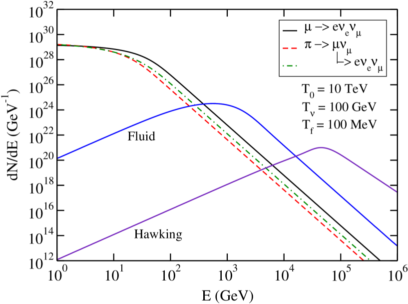
Figure 4: Same as Fig. 3 but with $T_{0}=10$ TeV.

The time-integrated spectra, starting at the moment when the Hawking temperature is 1 and 10 TeV, are shown in Figs. 3 and 4, respectively. The relative magnitudes and average energies reflect the trends seen in Figs. 1 and 2. At high energy the Hawking spectrum is proportional to $E^{-3}$ while all the others are proportional to $E^{-4}$, as was already pointed out in the previous sections. Obviously the greatest number of neutrinos by far are emitted at energies less than 100 GeV. The basic reason is that only about 5% of the total luminosity of the black hole is emitted directly as neutrinos. About 32% goes into neutrinos coming from pion and muon decay, about 24% goes into photons, with most of the remainder going into electrons and positrons.

6 Observability of the Neutrino Flux

We now turn to the possibility of observing neutrinos from a microscopic black hole directly. Obviously this depends on a number of factors, such as the distance to the black hole, the size of the neutrino detector, the efficiency of detecting neutrinos as a function of neutrino type and energy, how long the detector looks at the black hole before it is gone, and so on.

For the sake of discussion, let us assume that one is interested in neutrinos with energy greater than 10 GeV and that the observational time is the last 7.7 minutes of the black hole’s existence when its Hawking temperature is 1 TeV and above. As may be seen from Fig. 3, most of the neutrinos will come from the decay of directly emitted muons. Integration of eq. (31) from $E_{\rm min}=10$ GeV to infinity, and multiplying by 4 to account for both electron and muon type neutrinos and anti-neutrinos, results in the total number of

$$N_{\nu}=\frac{4}{750}\frac{m_{P}^{2}T_{f}}{E_{\rm min}^{3}}\approx 8\times 10^{31}\,.$$ (37)

This does not take into account neutrinos directly emitted from the fluid. For $E_{\rm min}=1$ TeV, for example, eq. (16) should be used in place of eq. (31) (see Fig. 3), and taking into account tau-type neutrinos too then yields a total number of about $3\times 10^{28}$. For an exploding black hole located a distance $d$ from Earth the number of neutrinos per unit area is

$$N_{\nu}(E>10\;{\rm GeV}) = 6700\left(\frac{1\;{\rm pc}}{d}\right)^{2}\;{\rm km}^{-2}\,,$$ (38)

$$N_{\nu}(E>1\;{\rm TeV}) = 2.5\left(\frac{1\;{\rm pc}}{d}\right)^{2}\;{\rm km}^{-2}\,.$$ (39)

Although the latter luminosity is smaller by three orders of magnitude, it has two advantages. First, 1/3 of that luminosity comes from tau-type neutrinos. Unlike electron and muon-type neutrinos, the tau-type is not produced by the decays of pions produced by interactions of high energy cosmic rays with matter or with the microwave background radiation. Hence it would seem to be a much more characteristic signal of exploding black holes than any other cosmic source (assuming no oscillations between the tau-type and the other two species). Second, the tau-type neutrinos come from near the neutrino-sphere, thus probing physics at a temperature of order 100 GeV much more directly than the other types of neutrinos.

What is the local rate density $\dot{\rho}_{\rm local}$ of exploding black holes? This is, of course, unknown since no one has ever knowingly observed a black hole explosion. The first observational limit was determined by Page and Hawking [11]. They found that the local rate density is less than 1 to 10 per cubic parsec per year on the basis of diffuse gamma rays with energies on the order of 100 MeV. This limit has not been lowered very much during the intervening twenty-five years. For example, Wright [12] used EGRET data to search for an anisotropic high-lattitude component of diffuse gamma rays in the energy range from 30 MeV to 100 GeV as a signal for steady emission of microscopic black holes. He concluded that $\dot{\rho}_{\rm local}$ is less than about 0.4 per cubic parsec per year. If the actual rate density is anything close to these upper limits the frequency of a high energy neutrino detector seeing a black hole explosion ought to be around one per year.

7 Conclusion

This paper has been a continuation of our previous work on a viscous fluid description of the radiation from microscopic black holes. In this paper we have calculated the spectra of all three flavors of neutrinos arising from direct emission from the fluid at the neutrino-sphere and from the decay of pions and muons from their decoupling at much larger radii and smaller temperatures. We should emphasize in particular the usefulness of distinguishing between the electron and muon-type neutrinos and the tau-type ones. The latter are much less likely to be produced by high energy cosmic rays. If the rate density of exploding microscopic black holes in our vicinity is anywhere close to the current limit based on gamma rays, it should be possible to observe them with present and planned large astrophysical neutrino detectors. Observation of high energy neutrinos, especially in conjunction with high energy gamma rays, may provide a window on physics well beyond the TeV scale.

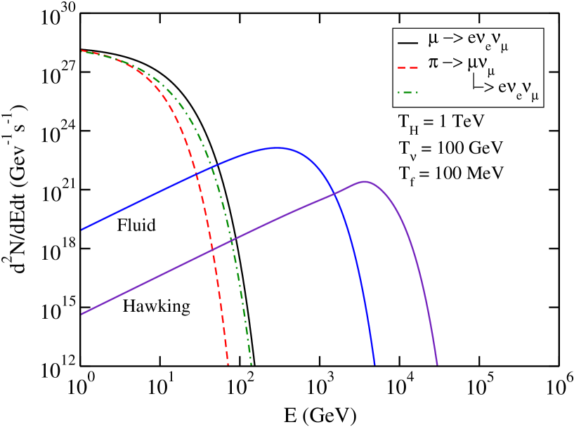
Figure 1: The instantaneous direct neutrino spectra emerging from the fluid with neutrino-sphere located at $T_{\nu}=100$ GeV compared to the direct Hawking radiation. Also shown are neutrinos arising from pion, direct muon and indirect muon decays at a decoupling temperature of $T_{f}=100$ MeV. Here the black hole temperature is $T_{H}=1$ TeV. All curves are for one flavor of neutrino or anti-neutrino.

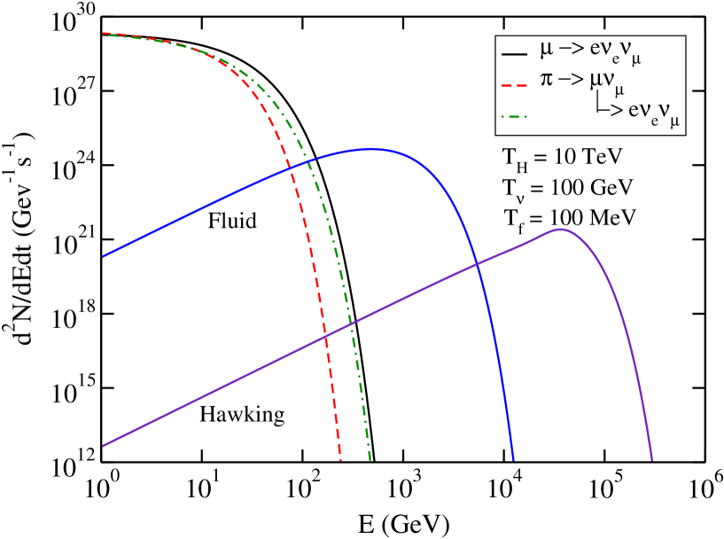
Figure 2: Same as Fig. 1 but with $T_{H}=1$ TeV.

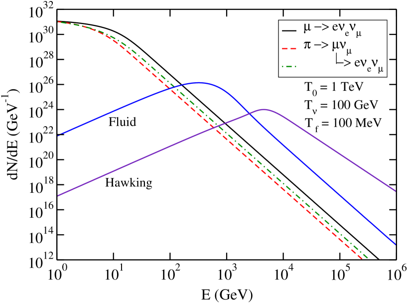
Figure 3: The time integrated neutrino spectra emerging from a microscopic black hole. Here the calculation begins when the black hole temperature is $T_{0}=1$ TeV. Either the direct Hawking radiation of neutrinos or the direct neutrino emission from a neutrino-sphere at a temperature of 100 GeV should be used. All curves are for one species of neutrino or anti-neutrino.

References

- [1] S. W. Hawking, Nature (London) 248, 30 (1974); Commun. Math. Phys. 43, 199 (1975).
- [2] A. F. Heckler, Phys. Rev. Lett. 78, 3430 (1997); Phys. Rev. D 55, 480 (1997).
- [3] J. Cline, M. Mostoslavsky, and G. Servant, Phys. Rev. D 59, 063009 (1999).
- [4] J. I. Kapusta, Phys. Rev. Lett. 86, 1670 (2001).
- [5] R. Daghigh and J. Kapusta, Phys. Rev. D 65, 064028 (2002).
- [6] J. H. MacGibbon and B. R. Webber, Phys. Rev. D 41, 3052 (1990); J. H. MacGibbon, ibid. 44, 376 (1991).
- [7] F. Halzen, B. Keszthelyi and E. Zas, Phys. Rev. D 52, 3239 (1995).
- [8] D. N. Page, Phys. Rev. D 13, 198 (1976); ibid. 14, 3260 (1976); 16, 2402 (1977).
- [9] W. G. Unruh, Phys. Rev. D 14, 3251 (1976).
- [10] N. Sanchez, Phys. Rev. D 18, 1030 (1978).
- [11] D. N. Page and S. W. Hawking, Astrophys. J. 206, 1 (1976).
- [12] E. L. Wright, Astrophys. J. 459, 487 (1996).