Critical review of the results of the Homestake solar neutrino experiment

The radiochemical experiment in the Homestake mine was designed to measure the solar neutrino flux through the detection of ${}^{37}Ar$ produced in the reaction $\nu_{e}+^{37}Cl\longrightarrow e^{-}+^{37}Ar$. The comparison between this measurement and the theoretical predictions from solar models evidences a substantial disagreement. I reanalyzed the data evidencing a bias with high statistical significance and suggesting a new interpretation of the data.

1 Introduction

The Homestake chlorine experiment has been running for over 20 years providing measurements of a portion of the solar neutrino flux. A detailed description of the experimental apparatus and of the analysis is given in Cleveland et al. (1998) and Bahcall (1989).
Briefly, the experiment consists of about 133 tons of ${}^{37}Cl$ in the form of $C_{2}Cl_{4}$ located in a tank in the Homestake mine. The solar neutrinos induce the reaction $\nu_{e}+^{37}Cl\longrightarrow e^{-}+^{37}Ar$ and the resulting ${}^{37}Ar$ is extracted and put into proportional counters, that measure energy and timing of each decay. The ${}^{37}Ar$ atoms are counted observing the $2.82\,\mathrm{keV}$ Auger electrons from the electron capture with a half life of $35.04\mathrm{d}$. The Auger electrons are selected by appropriate cuts on the rise time and selecting an energy window around the peak.
A run results in a time series of decays that is fit to the exponential decay of ${}^{37}Ar$ plus a decaying background. The ${}^{37}Ar$ production rate and the background level in each run are obtained by maximizing the probability of obtaining the given time series with a maximum likelihood technique optimized for low counting rate Cleveland et al. (1983). The same fit gives the ”$1\sigma$” errors on rate and background interpreted as $68\%$ confidence range. The results are presented separately for each run, that covers approximately two months of data taking.
In Cleveland et al. (1998) the data are presented as in the past (see Bahcall (1989)) in a list of single run analysis obtained using tight cuts on the rise time and on the energy window to optimize the dominant statistical error. Alternatively the data are selected with loose cuts on the rise time and on the energy window to reduce the systematic errors and a global likelihood analysis is applied to all of them. The final measurement of the neutrino flux is based on this latter analysis and therefore on data that are not presented in detail. Nevertheless, as several papers in the past Bahcall et al. (1987)-Bieber et al. (1990)-Krauss (1990)- Filippone & Vogel (1990)-Morrison (1992) and references therein, the single run results will be reanalyzed to verify their consistency with the hypothesis of constant flux.
This hypothesis has been challenged in the past by claims that the flux is correlated with the sun spot number or other parameter of solar activity or noticing that the fluxes measured over different time intervals differ significantly.
I performed the hypothesis testing of constant flux by calculating the $\chi^{2}$ of the distribution after having estimated the run errors. That results in a very poor agreement with the original hypothesis.
Error independent analysises were also performed using the Smirnov and Kolmogorov hypothesis tests and using rank order statistic analysises.
These show the signal and the background levels to be strongly correlated.
Furthermore the average fluxes and the hypothesis tests are calculated separately for different partitions of the run set according to the background level rank. The result strongly suggests a bias in the data and a very bad $\chi^{2}$ for the high background subset.
Based on this analysis, I give an alternative higher estimation of the flux.

2 Data and errors

The data analyzed in this paper are presented in Cleveland et al. (1998) for $N_{T}=108$ runs in the following format: run start time, run stop time, run average time (accounting for the decay of ${}^{37}Ar$ in the detector), production rate of ${}^{37}Ar$ resulting from the fit in atom per day, lower ”$1\sigma$” error (68% confidence range) on the production rate, higher ”$1\sigma$” error (68% confidence range) on the production rate, counter background resulting from the fit in count per day, lower ”$1\sigma$” error (68% confidence range) on the counter background, higher ”$1\sigma$” error (68% confidence range) on the counter background. These data are presented in Fig.1 for the production rate and in Fig.2 for the background.
In testing an hypothesis (for example production rate $p$ constant), it is necessary to assign an error to the rate measurement of each run. Previous analysis have devised different estimation of errors: equal on all runs, implicit in using rank-order statistic Bahcall & Press (1991), average of lower and higher errors Bahcall et al. (1987), the larger of the two Bahcall (1989)-Bieber et al. (1990)-Krauss (1990), calculated by rate and rate errors Filippone & Vogel (1990). All these estimations seems incorrect.
It is just the case to recall that if a measurement of a Poisson process of average $\mu$ is $n$, the error is $\sqrt{\mu}$ and not $\sqrt{n}$. This last estimation is approximately correct only for large $n$, that is in gaussian approximation. If only a single measurement is available, the best estimation of $\mu$ is $n$ and the two approaches coincide, but if several measurements are available, giving an estimation $\tilde{\mu}$ of $\mu$, the best estimation of the errors on the single measurement is $\sqrt{\tilde{\mu}}$.
Furthermore, the combination of a Poisson process of average $\mu$ and a binomial distribution due to an efficiency $\epsilon$ is a Poisson process of average $\mu\epsilon$. The errors on the production rate $p$ reported by the fit refer to the estimation of $p$ in the single run, while the best estimation $\tilde{p}$ makes use of all runs. Therefore, in absence of background counts, zero non-solar neutrino production rate and equal efficiency $\epsilon$ for each run, the average counts expected in run $i$ of duration $\Delta t_{i}$ are $n_{i}={\tilde{p}}\epsilon\Delta t_{i}^{eff}$, where $\Delta t_{i}^{eff}=(1-\exp(-\frac{\Delta t_{i}}{\tau_{{}^{37}Ar}}))\tau_{{}^{37}Ar}$ is the effective run time accounting for ${}^{37}Ar$ decay. Its error is $\sqrt{n_{i}}=\sqrt{\tilde{p}\epsilon\Delta t_{i}^{eff}}$ that gives an error on the rate $\sigma(\tilde{p})=\sqrt{\frac{\tilde{p}}{\epsilon\Delta t_{i}^{eff}}}$. Cleveland et al. (1983) reports that the efficiency is constant and equal to $\epsilon=0.95\times 0.96\times 0.327=0.298$.
If the non-solar neutrino rate is non-zero, the Poisson process under measurement is the sum of two distinct Poisson processes, the solar neutrino rate, $p_{S}$, and the non-solar neutrino rate $p_{i,NS}$, that is supposed known. The measurement gives an estimation ${\tilde{p}_{i}}={\tilde{p}_{S}}+p_{i,NS}$, from which ${\tilde{p}_{S}}={\tilde{p}}-p_{NS}$ (the true known value of $p_{NS}$ is used). That gives $\sigma_{i}^{2}(p_{S})=\sigma^{2}(\tilde{p})+\sigma_{i}^{2}(p_{NS})=\sigma^{2}(\tilde{p}_{S})+2\sigma_{i}^{2}(p_{NS})$, that is $\sigma_{i}(\tilde{p}_{S})=\sqrt{\frac{\tilde{p}_{S}+2p_{i,NS}}{\epsilon\Delta t_{i}^{eff}}}$.
In presence of background, the signal can be identified from the decay time of the atoms. Following a hint in Bahcall (1989), the background measurement stems from the counting in the signal free region at time larger compared to $\tau_{{}^{37}Ar}$, while the signal is measured from the counting within a few $\tau_{{}^{37}Ar}$. The statistical effect of the background can be evaluated expressing the background in term equivalent to signal rate and then applying the same approach used for the non solar rate component. The background induced rate is $\tilde{p}_{bk}=\frac{b_{i}\tau_{{}^{37}Ar}}{\epsilon\Delta t^{eff}_{i}}$, where $b_{i}$ is the background rate. The underlying assumption is that the contribution of the background to the signal measurement is concentrated in $\tau_{{}^{37}Ar}$.
With these definitions the total error on the solar rate is $\sigma_{i}(\tilde{p}_{S})=\sqrt{\frac{\tilde{p}_{S}+2p_{i,NS}+2\tilde{p}_{i,bk}}{\epsilon\Delta t_{i}^{eff}}}$.
It is apparent that, in order to use this errors to calculate anything relevant, an estimation of the rate must be already available. That is obtained through the unweighted average (actually weighted only through the effective run time length)

$$\tilde{p}_{uw}=\frac{\sum_{i}p_{i}\Delta t_{i}^{eff}}{\sum_{i}\Delta t_{i}^{eff}}.$$ (1)

The weighted average is instead obtained as

$$\tilde{p}=\frac{\sum_{i}\frac{p_{i}\Delta t_{i}^{eff}}{\sigma_{i}^{2}(\tilde{p})}}{\sum_{i}\frac{\Delta t_{i}^{eff}}{\sigma_{i}^{2}(\tilde{p})}}.$$ (2)

3 Hypothesis testing

The hypothesis of constant flux or, more generally, of consistency of the data set can be tested in several ways Frodesen et al. (1979)-Eadie et al. (1971).
The Pearson’s $\chi^{2}$ method quantifies the consistency of the constant flux hypothesis making use of the errors on the full sample, calculating

$$\chi^{2}(N-1)=\sum_{i}\left(\frac{p_{i}-\tilde{p}}{\sigma(p_{i})}\right)^{2}$$ (3)

where N is the number of data points.
Partitioning the data set in two subsamples A and B, the same approach can be repeated on each subsample as long as the estimator $\tilde{p}$ is replaced by the subsample estimator $\tilde{p}^{A(B)}$. A test of compatibility between the two samples is obtained estimating the probability of the difference between the two estimators.
The disadvantage of this approach is that it strongly relies on the exact evaluation of the errors. As discussed previously the presence of background creates some ambiguity in defining them.
Alternatively we can assume that all the data have the same weights and employ the hypothesis test of Kolmogorov and Smirnov. The test requires to order the N observation on the variable $p$ in ascending order ($x_{1}\cdots x_{N}$) and build their cumulative distribution

$$S_{N}(x)=\left\{\begin{array}[]{ll}0&x<x_{1}\\ \frac{i}{n}&x_{i}\leq x<x_{i+1}\\ 1&x>x_{N}\\ \end{array}\right.$$

This distribution is compared with the cumulative distribution function $F(x)$ occuring for a Poisson process at the constant rate determined through the weighted average. In principle the test is applicable only if the comparison function has no parameter determined by the data themselves; that is not our case but it is fair to assume that one parameter determined out of a large data sample will have little influence on its outcome.
The distance between the experimental and theoretical cumulative distributions is calculated in two different metrics: the first, named after Kolmogorov, is

$$D_{N}=max_{x}|S_{N}(x)-F(x)|,$$

the second, named after Smirnov, is

$$W^{2}_{N}=\int_{-\infty}^{+\infty}(S_{N}(x)-F(x))^{2}dF(x).$$

The distribution functions of $D_{N}\sqrt{N}$ and $W^{2}N$ can be calculated and are available as analytical formulae, tables or recurrence relations implemented by library routines.
The same approach and the same formulae allows the comparison between two set of data to verify if they come from the same original distribution. The distance between the cumulative distributions of two samples of size M and N is, after Kolmogorov,

$$D_{NM}=max_{x}|S_{N}(x)-S_{M}(x)|$$

where $D_{NM}\sqrt{MN/(M+N)}$ has the same probability distribution as $D_{N}\sqrt{N}$ and, after Smirnov,

$$W^{2}_{NM}=\int_{-\infty}^{+\infty}(S_{N}(x)-S_{M}(x))^{2}d\left[\frac{NS_{N}(X)+MS_{M}(X)}{N+M}\right]$$

where $W^{2}_{NM}(MN/(M+N))$ has the same probability distribution as $W_{N}^{2}N^{2}$. The test is exact because there are no estimated parameters.

3.1 The full data sample

The previous hypothesis tests applied to the full data sample under the hypothesis of constant flux give the following probabilities:

$$P(\chi^{2})=0.33\%$$

$$P(D_{N})=3.62\%$$

$$P(W^{2}_{N})=2.79\%$$

The smallest one ($\chi^{2}$) has the limit of relying heavily on a delicate procedure of error estimation. The others are more robust but not small enough to be conclusive.

Figure 1: Solar neutrino rate with the Homestake experiment on a run basis.

Figure 2: Background in the Homestake chlorine experiment on a run basis.

4 Rank measure of association

Another approach to the data is studying the correlation between the measured production rate in each run and another run dependent quantity. The candidate quantities are the run epoch, the effective run time length and the background rate. Alternatively any quantity defined versus the time epoch can be used. In Bahcall & Press (1991), Krauss (1990), Bieber et al. (1990) several sun’s activity dependent quantities are used, e.g. the mean sunspot number.
An estimation of correlation can be done using the standard correlation coefficient as in Krauss (1990) according to Press et al. (1986) or using rank-order statistic as in Bahcall & Press (1991). The latter is more robust because it makes no assumption on the underlying distributions nor on the data errors. As suggested in Bahcall & Press (1991) and described in Press et al. (1986) the rank statistical tests of Spearman rank-order correlation coefficient and Kendall’s $\tau$ are applied.
The principle is that if two quantities labelled by run index are rank ordered, the more uniform is the resulting scatter plot the less the two quantities are correlated.
In Fig.3, the background rate is plotted versus the ${}^{37}Ar$ production rate, as well as the corresponding rank ordered quantities. The rank ordered plot shows a denser diagonal band suggesting a significant anticorrelation.

4.1 The full data sample

The Spearman and Kendall tests are applied to the full data sample measuring the correlation between the ${}^{37}Ar$ production rate and the run epoch ($t_{r}$), the effective run time length ($t_{eff}$) and the background rate (back). The result is expressed as the probability to obtain the observed correlation parameter from two uncorrelated distributions:

	$t_{eff}$	$t_{r}$	back
Spearman $r_{s}$	4.95%	2.09%	$9.5\,10^{-3}$%
Spearman D	5.15%	2.04%	$14.3\,10^{-3}$%
Kendall	5.76%	1.88%	$14.9\,10^{-3}$%

From this table it is apparent that there is little (anti)-correlation between the Argon production rate and $t_{eff}$, a little more with the run epoch and a very strong one with the background level, that is visible in Fig.3. This correlation has no physical justification and has never been noticed before. Its strenght is comparable to the strongest correlation identified in previous papers Krauss (1990), Bahcall & Press (1991), Bieber et al. (1990).
It suggests that the analysis algorithm decreases the signal in presence of background and therefore that the average production rate is underestimated.

Figure 3: a) Background rate versus ${}^{37}Ar$ production rate b) Background rate rank versus ${}^{37}Ar$ production rate rank. In the null hypothesis of no correlation, the points should be uniformly distributed.

5 Partitioning the data set

The previous results provide strong suggestions that the ${}^{37}Ar$ production rate is anticorrelated with the background and that the overall consistency of the data under the hypothesis of constant flux is poor. Partitioning the data set in two subsets might help to gain more understanding on this disagreement.
To limit the arbitrariness of the partition, we consider the run set ranked according to the background rate and, for each number $1\leq N<N_{T}$, the partition in the two sets including the runs with the $N$ lower background rate and the runs with the $N_{T}-N$ higher background rate. That gives $N_{T}-1$ partitions in two sets.
For each set in each partition the average production rate is recalculated and the previous hypothesis tests are applied as well as the rank order tests. The hypothesis tests are applied also on the pair of sets of each partition to estimate the probablity that they come from the same constant distribution.
In Fig.4-4-4-4 the test and rank probabilities are plotted versus the background rate ranked run number. In Fig.5 the probabilities of low and high background ranked runs coming from the same constant distribution are plotted and in Fig.6 the average ${}^{37}Ar$ production rate for the two sets is shown.
What is apparent is that when the hypothesis and the rank tests are restricted to the lower two third of the runs (about 70), the experimental data are coherent with the hypothesis of constant ${}^{37}Ar$ production rate and the average value is constant with the run rank cut. Also the upper third of the runs, albeit less clearly, is a data set coherent with the hypothesis of constant ${}^{37}Ar$ production rate even if the average ${}^{37}Ar$ production rate depends on the run rank cut.
The plot in Fig.5 demonstrate that the probability that the two complementary sets belong to the same distributions reaches a minimum around a value of 70.
The most natural interpretation is that the low and high background sets come from two distinct populations with different averages. The low background population is highly coherent and unbiased and therefore gives the most reliable estimate of the ${}^{37}Ar$ production rate. The high backgorund population is less coherent, as it is to be expected if the measurement of the production rate is biased by the background, and does not provide a clear measurement of the average.

6 Conclusion

The conclusion from the previous results is that the analysis on the data from the Homestake experiment should be restricted to the subset of about two third of the runs with low background. The runs with large background should be discarded.
The somehow arbitrary choice of the cut in the backgorund rank adds a small uncertainties to the estimation of the ${}^{37}Ar$ production rate. Choosing $N=70$, using the weighted average as estimator and retaining the same systematic error of the original paper, the result is

$$0.566\pm 0.030(statistical)\pm 0.030(systematic)day^{-1}$$

or

$$3.03\pm 0.16(statistical)\pm 0.16(systematic)SNU$$

That is larger of almost three statistical standard deviation than the original result in Cleveland et al. (1998)

Figure 4: a) Probability of constant ${}^{37}Ar$ rate of the lowest N background runs for Smirnov (solid), Pearson (dashed) and Kolmogorov (dotted) b) Probability of constant ${}^{37}Ar$ rate of the highest $N_{T}-N$ background runs for Smirnov (solid), Pearson (dashed) and Kolmogorov (dotted) c) Probability of no correlation between ${}^{37}Ar$ rate and background of the lowest N background runs for Kendall (solid), Spearman D (dashed) and Spearman $r_{s}$ (dotted) d) Probability of no correlation between ${}^{37}Ar$ rate and background of the highest $N_{T}-N$ background runs for Kendall (solid), Spearman D (dashed) and Spearman $r_{s}$ (dotted) .

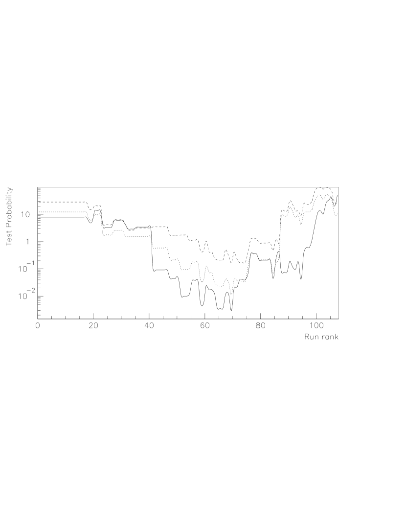
Figure 5: Probability of constant and equal ${}^{37}Ar$ rate between the lowest N and highest $N_{T}-N$ background runs for Smirnov (solid), Pearson (dashed) and Kolmogorov (dotted)

Figure 6: Weighted average of the ${}^{37}Ar$ rate of the lowest N (solid) and highest $N_{T}-N$ (dashed) background runs

References

- Bahcall (1989) Bahcall, J. 1989, Neutrino astrophysics (Cambridge: Cambridge University Press)
- Bahcall et al. (1987) Bahcall, J., Field, G., & Press, W. 1987, Astrophys. J., 320, L69
- Bahcall & Press (1991) Bahcall, J. & Press, W. 1991, Astrophys. J., 370, 730
- Bieber et al. (1990) Bieber, J. et al. 1990, Nature, 348, 407
- Cleveland et al. (1983) Cleveland, B. et al. 1983, NIMA, 214, 451
- Cleveland et al. (1998) —. 1998, Astrophys. J., 496, 505
- Eadie et al. (1971) Eadie, W., Drijard, D., James, F., Roos, M., & Sadoulet, B. 1971, Statistical methods in experimental physics (Amsterdam-New York-Oxford: North-holland)
- Filippone & Vogel (1990) Filippone, B. & Vogel, P. 1990, Phys. Lett. B, 246, 546
- Frodesen et al. (1979) Frodesen, A., Skjeggestad, O., & Tofte, H. 1979, Probability and statistics in particle physics (Bergen-Oslo-Tromso: Universitetforlaget)
- Krauss (1990) Krauss, L. 1990, Nature, 348, 403
- Morrison (1992) Morrison, D. 1992, in Inside the stars, IAU colloquium 137, ed. W. Weiss & A. Baglin, Astronomical society of the pacific volume 40, 100–107
- Press et al. (1986) Press, W., Flannery, B., Teukolsky, S., & Vetterling, W. 1986, Numerical Recipes: The Art of Scientific Computing (New York: Cambridge University Press)