Multi–Detector Multi–Component spectral matching and applications for CMB data analysis

Abstract

We present a new method for analyzing multi–detector maps containing contributions from several components. Our method, based on matching the data to a model in the spectral domain, permits to estimate jointly the spatial power spectra of the components and of the noise, as well as the mixing coefficients. It is of particular relevance for the analysis of millimeter–wave maps containing a contribution from CMB anisotropies.

1 Introduction

Mapping sky emissions at millimeter wavelengths, and in particular Cosmic Microwave Background (CMB) anisotropies, is one of the main objectives of ongoing observational effort in millimeter-wave astronomy. Sensitive balloon–borne and space–borne missions such as Archeops (Benoît et al, 2002b), Boomerang (, 2000), Maxima (Hanany et al., 2000) and MAP (Bennett et al., 1997) are currently in operating status, yielding a large amount of multi–detector and multi–frequency measurements. Within a few years, the Planck mission (Lamarre et al., 2000; Bersanelli & Mandolesi, 2000), to be launched by ESA in 2007, will observe the complete sky with $\sim 100$ detectors distributed in nine frequency bands ranging from 30 to 850 GHz. The main objective of these observations is the determination of the spatial power spectrum of CMB anisotropies. A secondary objective is identifying and mapping the emission from all contributing astrophysical processes.

The availability of several detectors operating in several bands makes it possible to devise new powerful data processing schemes. In particular, by combining data from several detectors, it is possible to improve substantially the signal-to-noise ratio (by weighted averaging) and to separate several foreground components (possibly of astrophysical interest in their own right) from the CMB by component separation methods. Component separation, however, typically requires a good knowledge of the transfer function connecting a multi-component sky to multi-detector maps.

This paper proposes to use spectral matching as a new approach to processing multi-detector multi-component (MDMC) data, in which all the information needed to estimate the spatial power spectra of components and/or to separate them is sought in the data structure itself. The method works with or without prior detector calibration and gives access to spatial power spectra in a straightforward way; it is statistically efficient (being a maximum likelihood technique) and computationally efficient (working with a small set of sufficient statistics rather than with original maps).

This paper is organised as follows. The idea of spectral estimation via multi–detector multi–component spectral matching is introduced in section 2. Section 3 describes the technique in more detail, connects it to a maximum likelihood method, and discusses the specific implementations. Section 4 is devoted to evaluating the performance of the method on synthetic Planck HFI observations. We discuss the method and extensions in section 5.

2 The multi-detector multi-component framework

Multi-detector CMB measurements can be modeled as resulting from the superposition of multiple components. Statistically efficient data processing should coherently exploit this MDMC structure.

The sky emission at millimeter wavelengths is well modeled at first order by a linear superposition of the emissions of a few processes: CMB anisotropies, thermal dust emission, thermal Sunyaev Zel’dovich (SZ) effect, synchrotron emission, etc. The observation of the sky with detector $d$ is then a noisy linear mixture of $N_{c}$ components:

$$y_{d}(\theta,\phi)=\sum_{j=1}^{N_{c}}A_{dj}s_{j}(\theta,\phi)+n_{d}(\theta,\phi)$$ (1)

where $s_{j}$ is the emission template for the $j$th astrophysical process, herein referred to as a source or a component. The coefficients $A_{dj}$ reflect emission laws and detector properties while $n_{d}$ accounts for noise. For simplicity, we neglect for the moment beam effects, postponing the discussion to section 5.

Quantities of prime interest are spatial power spectra. For the $j$-th component, at frequency $\vec{\ell}$, this is:

$$C_{j}(\vec{\ell})=\langle|s_{j}(\vec{\ell})|^{2}\rangle$$ (2)

where $\langle\cdot\rangle$ denotes the expectation operator and $\vec{\ell}$ indexes either a Fourier mode or an $(\ell,m)$ mode.

In practice, power spectra are estimated by averages over bins:

$$C_{j}(q)=\frac{1}{n_{q}}\sum_{\vec{\ell}\in\mathcal{D}_{q}}C_{j}(\vec{\ell}).$$ (3)

where $q=1,\ldots,Q$ is the spectral bin index, $\mathcal{D}_{q}$ is the set of frequencies contributing to bin $q$ and $n_{q}$ is the number of such frequencies. Typical bins can be bands $\ell_{\rm min}\leq\ell<\ell_{\rm max}$ extending over a range of one to tens of $\ell$ values.

Multi-detector power spectrum

Since we focus on jointly processing the maps from all detectors, it is convenient to stack $y_{1},\ldots,y_{N_{d}}$ into a single $N_{d}\times 1$ vector $Y$. Then, the set of eqs. 1 for all $N_{d}$ detectors is more compactly written in matrix–vector form as:

$$Y(\theta,\phi)=AS(\theta,\phi)+N(\theta,\phi)$$ (4)

with a so called $N_{d}\times N_{c}$ ‘mixing matrix’ $A$. In Fourier space, this equation reads

$$Y(\vec{\ell})=AS(\vec{\ell})+N(\vec{\ell}).$$ (5)

The power spectrum of process $Y$ is represented by the $N_{d}\times N_{d}$ spectral density matrix $\langle Y(\vec{\ell})Y(\vec{\ell})^{\dagger}\rangle$ where $\cdot^{\dagger}$ denotes transpose-conjugation. Its average over bins

$$R_{Y}(q)=\frac{1}{n_{q}}\sum_{\vec{\ell}\in\mathcal{D}_{q}}\langle Y(\vec{\ell})Y(\vec{\ell})^{\dagger}\rangle\ \ \ \ (q=1,\ldots,Q)$$ (6)

will also be referred to as a spectral density matrix. According to the linear model (1), it is structured as:

$$R_{Y}(q)=AR_{S}(q)A^{\dagger}+R_{N}(q)\ \ \ \ (q=1,\ldots,Q)$$ (7)

with $R_{S}(q)$ and $R_{N}(q)$ defined similarly to $R_{Y}(q)$. Statistical independence between components implies:

$$R_{S}(q)=\mathrm{diag}\left(C_{1}(q),\ldots,C_{N_{c}}(q)\right).$$ (8)

For the sake of exposition, we assume that the noise is uncorrelated, both across detectors and in space, so that the noise structure is described by $N_{d}$ parameters:

$$R_{N}(q)=\mathrm{diag}\left(\sigma_{1}^{2},\ldots,\sigma_{N_{d}}^{2}\right).$$ (9)

Parameter extraction by spectral matching

The MDMC model, as defined by eqs. (7-8-9), depends on a set $\{R_{Y}(q)\}$ of $Q$ spectral density matrices, which in turn depend on $\{A,C_{j}(q),\sigma_{d}^{2})\}$, amounting to $N_{d}\times N_{c}+Q\times N_{c}+N_{d}$ scalar parameters. However, the number of independent correlations in $Q$ spectral density matrices is $Q\times N_{d}(N_{d}+1)/2$ (since each matrix is real symmetric). This later number is (in general) higher than the former.

With this in mind, our proposal can be summarized as ‘MDMC spectral matching’, meaning: estimate all (or parts of) the parameters $\{A,C_{j}(q),\sigma_{d}^{2})\}$ by finding the best match between $\{R_{Y}(q)\}$, as specified by (7-8-9), and a set of $Q$ ‘empirical spectral density matrices’ $\{\widehat{R}_{Y}(q)\}$:

$$\widehat{R}_{Y}(q)=\frac{1}{n_{q}}\sum_{\vec{\ell}\in\mathcal{D}_{q}}Y(\vec{\ell})Y(\vec{\ell})^{\dagger}\ \ \ \ (q=1,\ldots,Q)$$ (10)

which are the natural non parametric estimates of the corresponding $R_{Y}(q)$.

Some preliminary comments about the MDMC spectral matching approach are in order.

Parameter choice:   There is a lot of flexibility in the choice of parameters over which to minimize the spectral mismatch. By selecting different sets of parameters, different goals can be achieved. For instance, we may assume that matrix $A$ and the noise spectrum $R_{N}(q)$ are known so that the mismatch is minimized only with respect to the binned spectra $C_{i}(q)$ of all components: the method appears as a spectral estimation technique which does not require the explicit separation of the observed maps into component maps. Another important example, as illustrated in section 4, consists in including matrix $A$ among the free parameters. Then, the method works as the so-called ‘blind techniques’, and permits the measurement of the emission law of the components, or the cross calibration of detectors.

Degeneracies:   A key issue in spectral matching is whether or not matrix $A$ can be uniquely determined from the data only. When all parameters $\{A,C_{j}(q),\sigma_{d}^{2}\}$ are allowed to be adjusted, there are at least two clear indeterminations. First, the ordering (or numbering) of the components in the model is immaterial: matrix $A$ cannot be recovered better than up to column permutation on the sole basis of a spectral match. Second, a scalar factor can be exchanged, for each component $j$, between the $j$th column of $A$ and $C_{j}(q)$. These scale factors cannot be determined from the data themselves.

Another trivial case of indetermination is when two columns of $A$ corresponding to physically distinct components are proportional. In this case, the sum of the two appears in the model as one single component. The identifiability of the other components is not affected.

A more severe degeneracy occurs if any two components have proportional spectra. In this case, as is known from the noiseless case (Pham & Garat, 1997), only the space spanned by the corresponding columns of $A$ can be determined in a spectral match with $A$ as a free parameter. In this case however, the identifiability of the other components is unchanged, with no impact on the accuracy of component separation with a Wiener method (sec. 5). The key point to remember is that spectral matching requires spectral diversity to separate components associated with unknown columns of $A$.

Maximum likelihood:   Section 3.1 explains why ‘spectral matching’ corresponds to maximum likelihood estimation. This happens in a Gaussian stationary model with smooth (actually: constant over bins) spectra. In such a model the likelihood of the observations is a measure (12) of spectral matching. Since the likelihood then depends on the data only via the empirical spectral density matrices, the massive data reduction gained from replacing the observations by a (usually) much smaller set of statistics (the empirical spectral density matrices $\widehat{R}_{Y}(q)$) is obtained without information loss.

Comparison with component separation:   It is interesting to compare spectral matching to techniques based on prior explicit component separation.

Producing a CMB map as free as possible from foreground and noise contamination is the objective of the component separation step, in which maps obtained at different frequencies are combined to maximize the signal to noise ratio (where noise includes also foreground contamination).

The usual approach for taking advantage of multi–detector measurements can be summarised as: first, form estimates $\widehat{s}_{j}(\vec{\ell})$ of component maps $s_{j}(\vec{\ell})$ (via component separation), second, estimate the spectrum of each component $j$ by averaging within bins:

$$\widehat{C}_{j}(q)=\frac{1}{n_{q}}\sum_{\vec{\ell}\in\mathcal{D}_{q}}|\widehat{s}_{j}(\vec{\ell})|^{2}$$ (11)

with, possibly, some post-processing of the power spectrum estimates.

This method suffers from two difficulties. First, the best component separation methods typically require the prior knowledge of the statistical properties of the components (including the CMB power spectrum) and of the noise. Second, recovered maps contain residuals (including noise) which contribute to the total power, biasing the spectrum estimated on the map, unless the power spectrum of these residuals can be estimated accurately and subtracted for de–biasing.

In contrast our approach takes the reverse path. The first step is the estimation of the spectrum for the multi–detector map (which takes the form of a sequence of spectral density matrices). This first step preserves all the joint correlation structure between maps. In essence, the second step (spectral matching) amounts to resolving the joint power spectrum into spectra of individual components.

Hence, instead of first separating component maps and then computing power spectra, we first compute the multivariate power spectrum and then separate component spectra.

3 MDMC spectral matching in practice

The implementation of MDMC spectral matching is now described in more detail. Section 3.1 introduces the spectral matching criterion; section 3.2 describes the EM algorithm for its optimization; section 3.3 describes a complementary technique for fast convergence.

3.1 Maximum likelihood spectral matching

Any reasonable measure of mismatch between the empirical density matrices $\{\widehat{R}_{Y}(q)\}$ and their model counterparts $\{\widehat{R}_{Y}(q;\theta)\}$ could be used to compute estimates of a $\theta$ parameter. In order to get good estimates, however, one should use a mismatch criterion derived from statistical principles. Such a derivation can be based on the statistical distribution of the Fourier coefficients of a stationary process which are (at least asymptotically in the data size) normally distributed, uncorrelated, with a variance proportional to the power spectrum (Whittle approximation, see appendix B). Thus, the likelihood of the observations can be readily expressed in terms of spectral density matrices. Appendix B outlines how the (negative) log-likelihood of the data then is (up to irrelevant factors and terms) equal to

$$\phi(\theta)=\sum_{q=1}^{Q}n_{q}\ D\left(\widehat{R}_{Y}(q),R_{Y}(q;\theta)\right)$$ (12)

where $D(\cdot,\cdot)$ is a measure of divergence between two positive $n\times n$ matrices defined by

$$D(R_{1},R_{2})=\mathrm{tr}\left(R_{1}R_{2}^{-1}\right)-\log\det(R_{1}R_{2}^{-1})-n.$$ (13)

It can be seen that $D(R_{1},R_{2})\geq 0$ with equality if and only if $R_{1}=R_{2}$. Thus spectral matching corresponds to maximum likelihood estimation in a stationary model. The minimizer of $\phi(\theta)$ is then a maximum likelihood estimate, and inherits the good statistical properties associated to it.

Only in an asymptotic framework can maximum likelihood procedures be proved to reach minimum estimation variance. It means that criteria which are equivalent to (12) are expected to have the same statistical quality as (12). In particular, criterion (12) can be replaced by a quadratic approximation: when each $\widehat{R}_{Y}(q)$ is close $R_{Y}(q;\theta)$, a second-order expansion of $D(\widehat{R}_{Y},R_{Y})$ yields

$$D_{2}\left(\widehat{R}_{Y},R_{Y}\right)=\mathrm{tr}\left(\widehat{R}_{Y}^{-1}(\widehat{R}_{Y}-R_{Y})\widehat{R}_{Y}^{-1}(\widehat{R}_{Y}-R_{Y})\right).$$ (14)

The resulting quadratic criterion is of particular interest when the unknown parameters enter linearly in $R_{Y}(q;\theta)$ (for instance when $A$ is known and $\theta$ only contains the binned power spectra of the components) since then criterion minimization becomes trivial. In this paper, however, we stick to using (12-13). Even though the divergence (13) may, in the general case, seem more difficult to deal with than its quadratic approximation (14), it actually lends itself to simple optimization via the EM algorithm (see section 3.2) thanks to its connection to the likelihood.

3.2 The EM algorithm

The expectation-maximization (EM) algorithm (Dempster et al., 1977) is a well known technique for maximizing the likelihood of statistical models which include ‘latent’ or ‘unobserved’ variables. It is well suited to our purpose by taking the components as the latent variables. The EM algorithm is iterative: starting from an initial value of the parameters, it performs a sequence of parameter updates called ‘EM-steps’. Each step is guaranteed to increase the likelihood of the parameters.

The spectral matching criterion (12) actually being a likelihood function in disguise, the EM algorithm can be used for its minimization. Each EM step is guaranteed to improve the spectral fit by decreasing $\phi(\theta)$.

We consider the regular EM algorithm, based on the Gaussian likelihood described in appendix B and taking as ‘latent variables’ the spectral modes $Y(\vec{\ell})$. The form of the EM steps immediately follows as sketched in appendix C and summarized by the pseudo-code.

Algorithm 1 The EM algorithm for minimizing the MDMC spectral mismatch $\phi(\theta)$ with respect to $\theta=\{A,C_{j}(q),\sigma_{d}^{2}\}$.

0:  Spectral density matrices $\widehat{R}_{Y}(1),\ldots,\widehat{R}_{Y}(Q)$

0:  Initial value of $\theta=\left\{A,C_{j}(q),\sigma_{d}^{2}\right\}$.

  Set $\widetilde{R}_{yy}(q)=\widehat{R}_{Y}(q)$ and $\widetilde{R}_{yy}=\sum_{q}\frac{n_{q}}{n}\ R_{yy}(q)$.

  repeat

     { E-step. Compute conditional statistics:}

     Set $R_{S}(q)=\mathrm{diag}(C_{j}(q))$ and $R_{N}=\mathrm{diag}(\sigma_{d}^{2})$

     for $q=1$ to $Q$ do

        $G(q)=(A^{\dagger}R_{N}^{-1}A+R_{S}(q)^{-1})^{-1}$

        $W(q)=G(q)A^{\dagger}R_{N}^{-1}$

        $\widetilde{R}_{ss}(q)=W(q)\widehat{R}_{Y}(q)W(q)^{\dagger}+G(q)$

        $\widetilde{R}_{sy}(q)=W(q)\widehat{R}_{Y}(q)$

     end for

     $\widetilde{R}_{ss}=\sum_{q=1}^{Q}\frac{n_{q}}{n}\ \widetilde{R}_{ss}(q)$

     $\widetilde{R}_{ys}=\sum_{q=1}^{Q}\frac{n_{q}}{n}\ \widetilde{R}_{ys}(q)$

     { M-step. Update the parameters:}

     $A=\widetilde{R}_{ys}\widetilde{R}_{ss}^{-1}$

     $C_{i}(q)=\left[\widetilde{R}_{ss}(q)\right]_{ii}$

     $\sigma_{d}^{2}=\left[\widetilde{R}_{yy}-\widetilde{R}_{sy}^{\dagger}\widetilde{R}_{ss}^{-1}\widetilde{R}_{sy}\right]_{dd}$

     Rescale the parameters (see text).

  until a convergence criterion is satisfied

It is worth mentionning that EM steps take such a regular structure when the parameters are $\theta=\{A,C_{j}(q),\sigma_{d}^{2}\}$. A slightly different form would result from a more constrained parameter set.

Recall that, as previously noted, there is a scale indetermination on each component’s spectrum when $\theta=\{A,C_{j}(q),\sigma_{d}^{2}\}$. We have found that this inherent indetermination must be explicitly fixed in order for EM to converge (this is the rescaling step in the last line of the pseudo-code). Our strategy is, after each EM step, to fix the norm of each column of $A$ to unity and to adjust the corresponding power spectra accordingly. This is an arbitrary choice which happens to work well in practice.

3.3 Non linear optimization

When applied to our data, the EM algorithm shows fast convergence in a first phase and then enters a second phase of slower convergence. This is due to the fact that some parameters (e.g. sub-dominant power spectra in some spectral domains) have a very small effect on the criterion. In order to reach the true minimum of $\phi(\theta)$, it appears necessary to complement EM with another minimization technique. The strategy is to use the straightforward EM algorithm to quickly get close to the minimum of $\phi(\theta)$ and then to complete the minimization using a dedicated minimization algorithm. This complementary algorithm can use a simple design thanks to the good starting point provided by EM.

The spectral mismatch criterion (12) can, in theory, be minimized by any optimization algorithm. However, the same effect which slows down EM in its final steps also makes the minimization of the mismatch criterion (12) difficult for any algorithm. In particular, simple gradient algorithms are unacceptably slow. Actually, we found that even conjugate gradient techniques cannot overcome this problem and had to resort to a quasi-Newton method. We have used the classic BFGS (Broyden-Fletcher-Goldfarb-Shapiro) algorithm (Luenberger, 1973). This technique minimizes an objective function by successive one-dimensional minimization (line searches). At each step, the direction for the line search is the gradient ‘rectified’ by the inverse of Hessian matrix. The BFGS technique is a rule to update an estimate of the inverse Hessian matrix at low computational cost.

4 Testing and Performance

We now turn to illustrating the applications and performance of our multi–detector multi–component spectral–matching method on a simple set of synthetic observations: three-component noisy linear mixtures featuring contributions from CMB anisotropies, dust emission, and SZ thermal emission. Unbiasedness and statistical uncertainties are investigated by a Monte–Carlo technique.

Five implementations of the method for different applications will be discussed:

1. a multi–component spatial power spectrum estimation assuming the mixing matrix is known,

2. a blind approach in which spatial power spectra, noise levels, and the emission laws of components are jointly estimated on the data,

3. a semi–blind approach where CMB and SZ emission laws are assumed to be known, and the emission law of the dust component (in addition to spatial power spectra and noise levels for all components) is estimated from the data,

4. an application for detector cross–calibration,

5. a Wiener–filter component separation using parameters estimated via blind spectral matching.

Finite beam effects are neglected for the present work, although they are not a fundamental limitation for our method (see sec. 5). For definiteness, we also assume here that the noise is white, although this assumption can be relaxed as well if needed.

4.1 Simulated data

Synthetic observations in six frequency bands identical to those of the Planck HFI are generated on $300\times 300$ pixel maps corresponding to a 12.5^∘ $\times$ 12.5^∘ field located at high galactic latitude. For each mixture realisation, synthetic components and noise are obtained as follows:

• The CMB component is a COBE-normalised, randomly generated realization of CMB anisotropies obtained using the spatial power spectrum $C_{\ell}$ predicted by the CMBFAST software (Zaldarriaga & Seljak, 2000) with $H_{0}=65$ km/s/Mpc, $\Omega_{m}=0.3$, $\Omega_{b}=0.045$, $\Lambda=0.7$.

• The galactic dust emission template is obtained from the 100 $\mu$m IRAS data in the sky region located around $\alpha=204^{\circ}$ and $\delta=11^{\circ}$. Bright stars are removed using a point source extracting algorithm. Residual stripes are cut out by setting to zero the contaminated Fourier coefficients. The Fourier modes suppressed in this way are randomly re-generated with a distribution obtained, for each mode, from the statistics of the other modes at the same scale in the IRAS map. This method preserves the (assumed) statistical azimuthal symmetry and general shape of the spatial spectrum.

• The thermal Sunyaev-Zel’dovich template is drawn at random from a set of 1500 SZ maps generated for this purpose using the software described in (Delabrouille et al., 2002).

• White noise at the level of the nominal per–channel Planck HFI values is added to the observations.

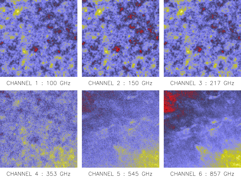
Figure 1: Simulated observations for six frequency bands

Synthetic observations are displayed in fig. 1. The general common pattern which can be seen in the lowest frequency channels is simulated CMB anisotropies, whereas the pattern of emission of interstellar dust as observed with IRAS dominates our 857 and 545 GHz maps. The contribution of the SZ effect, very sub-dominant, is not obviously visible on these maps.

$\nu$	100	143	217	353	545	857
CMB	0.889	0.926	0.896	0.275	0.0019	1.3$\times 10^{-7}$
dust	9$\times 10^{-5}$	6$\times 10^{-4}$	0.0082	0.215	0.687	0.938
SZ	0.0064	0.0032	2$\times 10^{-7}$	0.0044	0.00019	5.2$\times 10^{-8}$
noise	0.102	0.0727	0.108	0.536	0.320	0.0667

Table 1: Fraction of the power in each of the components

Table 1 gives, for each channel, the relative power of all components and of noise for a typical synthetic mixture (here ‘relative’ means: the sum of all powers is normalised to unity). Typical input templates for the three components can be seen in figure 6, left column.

4.2 Application 1: Spectral estimation

The first application is the estimation of component spatial power spectra. It is assumed that the mixing matrix is known, but that the noise level for each map is not known precisely. The set of parameters to be estimated from the data then is $\theta=\{C_{j}(q),\sigma_{d}^{2}\}$.

Component spectra are estimated on 32 ring-shaped domains for 5,000 different mixtures. The first 30 domains are equally spaced rings covering the lowest 60% of the spatial frequencies ($0<\ell/\ell_{\rm max}<0.6$), and the remaining two cover respectively $0.6<\ell/\ell_{\rm max}<0.8$ and $0.8<\ell/\ell_{\rm max}<1$. This choice of spectral domains is adapted to the assumed azimuthal symmetry of the spectra by the choice of ring-shaped domains, and has a large number of rings in the region where the signal is strong and where information from source spectra is relevant.

Figure 2: This figure shows the recovered spatial power spectrum $\ell^{2}C_{\ell}$ (crosses) compared to the exact band-averaged spectra (solid lines) for CMB (left), dust (middle), and Thermal SZ effect (right). These results correspond to a non-blind MDMC spectral estimation in which the mixing matrix $A$ is known. Vertical bars show the $1\sigma$ errors, and horizontal bars the spatial frequency range of each bin.

The result of the estimation of the spatial power spectrum of the three components in the relevant frequency range is shown in fig. 2. Errors on estimated spectra are obtained from the dispersion over the 5,000 distinct simulated observations. For the SZ effect, the spatial power spectrum is averaged into larger bins after parameter estimation to reduce the scatter of the measurements. The figure shows that, as expected, a low-variance unbiased power spectrum is obtained for all components without explicit separation of the observations into component maps. For the CMB, the measurement is sample (cosmic) variance limited at small spatial frequencies. Such an effect does not appear on the dust spectrum estimate because we use only one dust map in the Monte-Carlo.

4.3 Application 2: Blind parameter estimation

Let us now assume that the exact emission laws of all components are unknown. Then the full parameter set, to be estimated from the data, is $\theta=\{C_{j}(q),\sigma_{d}^{2},A\}$. Again, we estimate parameters on 5,000 different simulated data sets. For each run, the scale indetermination between mixing matrix columns and component power spectra is fixed by renormalising to the true value of $A$ at a single reference frequency (100 GHz for the CMB and thermal SZ effect, and 857 GHz for the dust). Error bars ($\pm 1\sigma$) for all parameters are computed from the distribution of the estimates over all simulated observations.

channel	100	143	217	353	545	857
RMS est. $\times 10^{-6}$	(29.1 $\pm$ 0.22)	(18.7 $\pm$ 0.13)	(12.85 $\pm$ 0.09)	(11.92$\pm$ 0.07)	(8.98 $\pm$ 0.05)	(4.97 $\pm$ 0.06)
RMS true $\times 10^{-6}$	29.11	18.70	12.86	11.93	8.980	4.970

Table 2: Comparison of true and estimated noise levels (RMS). The errors are obtained from the dispersion of results obtained using 10,000 different mixtures.

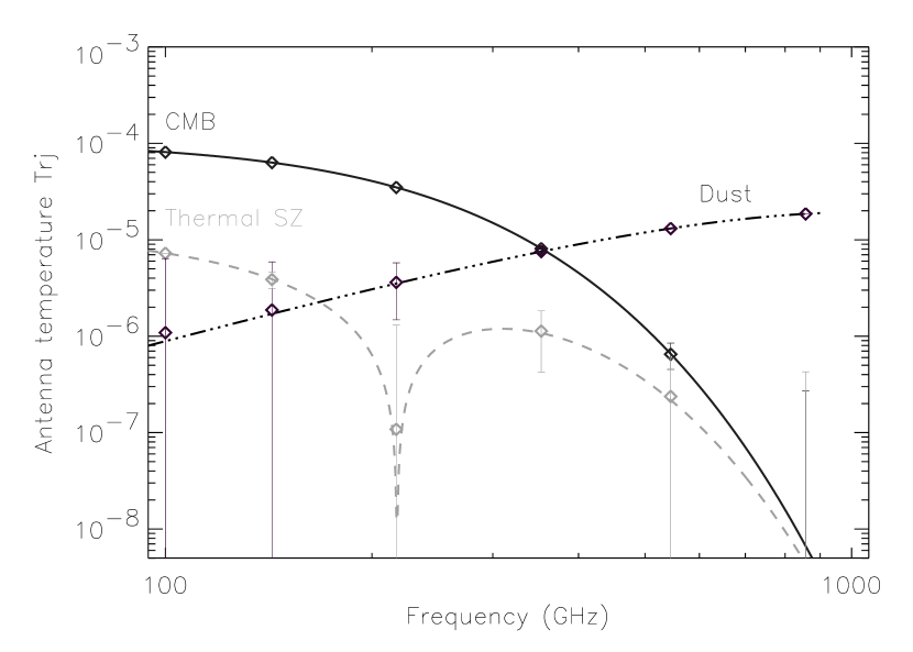
Figure 3: The figure shows the recovered emission laws of the components (diamonds) compared to the exact emission laws used in the simulations (solid lines). The errors are computed from the dispersion of the recovered values for 10,000 different synthetic mixtures.

Figure 3 displays recovered emission spectra (diamonds with 1$\sigma$ error bars) as compared to exact emission spectra (solid lines). Emission laws of all components are recovered with no significant bias. The CMB emission law is recovered very accurately at all frequencies except 857 GHz. The dust emission law is recovered quite accurately at high frequencies, less accurately at frequencies where it is very sub–dominant. The SZ effect emission shape, sub–dominant at all frequencies, is recovered with larger relative error bars. Because of the renormalisation, error bars for CMB and SZ vanish at 100 GHz, and the dust emission law error bar vanishes at 857 GHz.

Spatial power spectra, in turn, are also estimated. As shown in figure 4, CMB and dust spatial power spectra are recovered with good accuracy and no significant bias, almost as well as for the non–blind spectral estimation. The SZ power spectrum is also significantly constrained, although error bars are significantly larger than in the non-blind spectral estimation.

Figure 4: The figure —similar to fig. 2 but for blind spectral matching— shows the recovered power spectra of the components compared to exact ones (solid lines). The errors are computed from the dispersion of the recovered values for 5,000 different synthetic mixtures.

Finally, table 2 shows the estimates of the noise RMS as compared to true levels. Relative errors are below 2.5 % for all channels.

4.4 Application 3: Semi-blind parameter estimation

In our particular case, the emission laws of the CMB and of the SZ are known to almost perfect accuracy. Assume, however, that measuring the dust emission law is of particular interest. How much do we gain by forcing known emission laws to their true value, and estimating only the unknown dust emission spectrum?

channel	100	143	217	353	545	857
true dust em spectrum	0.3071	0.5902	1.2177	2.6106	4.5371	6.4288
relative error, blind approach	6.229	2.469	0.634	0.0662	0.00790	no values
relative error, semi-blind approach	2.623	1.056	0.285	0.0368	0.00725	no values

Table 3: Relative errors on dust emission law estimation. In the first case, all the elements of the mixing matrix are estimated (blind approach). In the second case, the columns of the mixing matrix which corresponds to the CMB and the thermal SZ components are fixed (semi-blind approach). Although the semi-blind approach does not improve significantly the determination of the dust spectrum at 545 GHz, the improvement is very significant (factors of two to three) at other frequencies.

We repeat the simulations described in 4.3, now fixing two columns of the mixing matrix, and estimating the third one (in addition to domain-averaged spatial spectra and noise levels). Table 3 compares quantitatively the relative errors on the resulting dust emission law. At low frequency (between 100 and 217 GHz), the accuracy of the estimation is improved by a factor of 2 to 3. At 353 GHz, the improvement is still noticeable, but at 545 GHz, where the dust emission begins to dominate, the blind and semi–blind approaches give similar errors. The use of partial prior information on the mixing matrix $A$ is thus useful here to improve the estimation of the entries of $A$ which contribute little relative power to the observations.

Figure 5: The figure shows the comparison of the quality of the blind and semi-blind power spectrum estimation of the components. The solid line displays the ratio between the size of the $1\sigma$ error in the semi–blind and in the non–blind spectral matching, showing that they are comparable to within simulation accuracy. In contrast, the dotted line shows the ratio between the size of the $1\sigma$ error in the blind and in the non–blind spectral matching, showing that some accuracy is lost when all components of the mixing matrix are adjusted as additional parameters.

In addition to this substantial improvement in estimating the unknown ‘dust column’ of $A$, the semi–blind approach is more efficient for estimating the SZ power spectrum than the full blind implementation. Figure 5 shows the comparison of the quality of spectral estimation in the blind and semi–blind approaches relative to the non-blind. To the precision of our Monte-Carlo tests (1–2% level on error bars), the semi–blind result is as accurate for this particular mixture as the non-blind estimate, significantly better than the blind result. As the semi–blind and the non–blind estimates give similar results, however, the actual enhancement in precision depends on details of the mixture and parametrization.

This comparison, however, shows that it is in general useful to exploit as much as possible reliable prior information. Our method is flexible enough to do so.

4.5 Application 4: Detector calibration

The mixing matrix $A$ depends not only on components (through emission spectra), but also on detectors (through frequency bands and optical efficiency). Mixing matrix coefficients $A_{dj}$, expressed in readout (rather than physical) units can be approximated by the product of a detector-dependent calibration coefficient $\alpha_{d}$ and an emission law $\epsilon_{j}(\nu)$:

$$A_{dj}\simeq\alpha_{d}\epsilon_{j}(\nu_{d})$$ (15)

where $\nu_{d}$ is the central observing frequency of detector $d$. Used on a data set from detectors observing in the same frequency band, the estimation of $A$ for any astrophysical component gives relative calibration coefficients between detectors. If in addition the emission law of at least one of the components is known (e.g. CMB anisotropies), the estimation of the mixing matrix provides a relative calibration across frequency bands. Finally, if among the components there is one with known emission spectrum and known amplitude (or known spatial power spectrum), absolute calibration can be obtained in the same way. For instance, it is not excluded that in the not-so-far future, a high resolution experiment dedicated to a wide-field point source survey in the millimeter range can be calibrated on CMB anisotropies(!).

4.6 Application 5: Component separation

The separation of astrophysical components by some kind of inversion of the linear system of equation 1 has been the object of extensive previous work. Popular linear methods are listed in appendix A. In a Gaussian model, the best inversion is obtained by the Wiener filter. This filter, however, requires the prior knowledge of the mixing matrix $A$, component spatial power spectra, and noise power spectra. As discussed by (Cardoso et al., 2002), our spectral–matching method yields all the parameters needed to implement a Wiener–based component separation on maps.

We compare the quality of component reconstruction using either the estimated parameter set $\theta=\{C_{j}(q),\sigma_{d}^{2},A\}$ or ‘true’ best-knowledge values.

Reconstructed maps.   Figure 6 illustrates the quality of map reconstruction by Wiener inversion. The first column displays the input components, the second column shows components recovered with the exact Wiener filter (computed from the true mixing matrix, ensemble averages of the noise, ensemble averages of CMB and SZ power spectra, and a $k^{-3}$ fit of the spatial power spectrum of the dust template). The third column displays the components recovered by Wiener inversion using estimated parameters. In both cases, CMB and dust emissions are recovered satisfactorily, but the SZ effect —strongly peaked and hence poorly suited to processing in Fourier space— remains noisy. Visually, both methods perform about as well.

Figure 6: Left: true templates used as inputs. Middle: templates recovered using the ‘true’ Wiener filter. Right: templates recovered using the blind separation.

Contamination levels.   The quality of the separation can be assessed by a measure of contamination levels, i.e. how much of the other components gets into a component’s map after separation.

The Wiener matrix, $W=[A^{t}R_{N}^{-1}A+R_{S}^{-1}]^{-1}A^{t}R_{N}^{-1}$, obtained with exact values of $A$, $R_{N}$ and $R_{S}$, differs slightly from its estimate $\widehat{W}$, computed with estimates ${\widehat{A}}$, ${\widehat{R}_{N}}$ and ${\widehat{R}_{S}(q)}$. Not only ${\widehat{R}_{S}(q)}$ differs from $R_{S}$ because it is an estimate, but also because it is a flat band-power approximation.

At each frequency, off-diagonal terms of $\widehat{W}A$ correspond to leakage of other components into one component’s estimate at spatial frequency $k$. Each panel of figure 7 refers to one component (CMB, dust and SZ), and shows the relative contribution of all components and of noise to the recovered map. Levels are relative to the true map, so that the contribution of a component to its own recovered map illustrates the spatial filtering induced by the Wiener inversion. The figure illustrates that the inversion done with blindly estimated parameters performs almost as well as the separation using exact values of the spectra and mixing matrix. Differences are typically much smaller than noise contamination, which is comparable with the blind and the non-blind approaches.

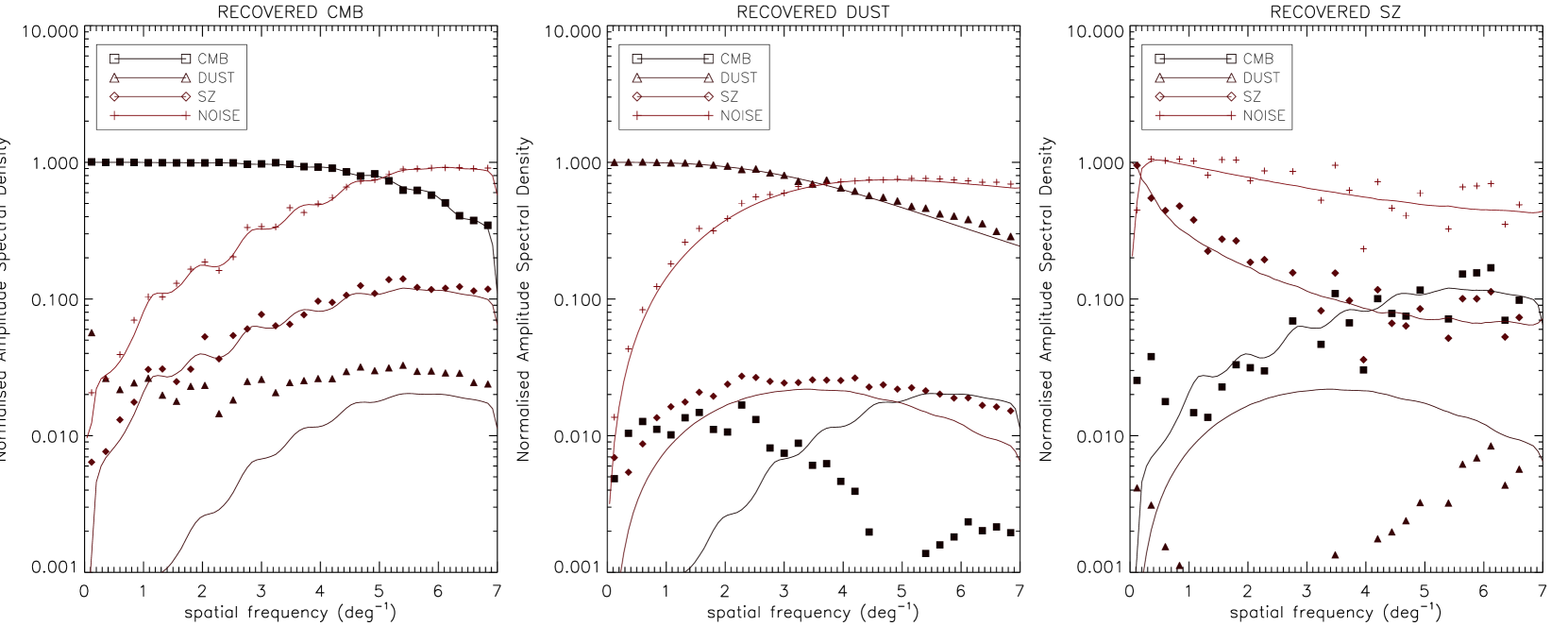
Figure 7: Contributions to the output map as a function of spatial frequency, relative to the true level of that component map. The left panel is for CMB, the middle panel for dust, and the right panel for the SZ effect. Results obtained with exact values of the mixing matrix, the spectra and noise levels are plotted as plain lines, and results obtained with the Wiener implementation using estimated parameters as diamonds.

5 Discussion

5.1 Related work on component separation

Explicit component separation has been investigated first in CMB applications by Tegmark & Efstathiou (1996), Bouchet & Gispert (1999), and Hobson et al. (1998). In these applications, all the parameters of the model (mixing matrix, noise levels, statistics of the components, including the spatial power spectra) are assumed to be known.

Recent research has addressed the case of an imperfectly known mixing matrix. It is then necessary to estimate it (or at least some of its components) directly from the data. For instance, Tegmark et al. assume power law emission spectra for all components except CMB and SZ, and fit spectral indices to the observations (Tegmark et al., 2000).

More recently, it has been proposed to resort to ‘blind source separation’ or ‘independent component analysis’ (ICA) methods. The work of Baccigalupi et al. (2000), further extended by Maino et al. (2002) implements a blind source separation method exploiting the non–Gaussianity of the sources for their separation. This infomax method, unfortunately, is not designed for noisy mixtures and can not deal with a frequency–dependent beam.

The idea to use spectral diversity and an EM algorithm for the blind separation of components in CMB observations was proposed first by Snoussi et al. (2001). This approach exploits the spectral diversity of components as in our MDMC spectral matching, but assumes the prior knowledge of the spatial power spectra of the components. Our approach extends further on this idea, with a lot more flexibility, and the new point of view that spatial power spectra are actually the main unknown parameters of interest for CMB observations.

Other reports of blind component separation in astronomical data include Nuzillard & Bijaoui (2000) and Funaro et al. (2001).

5.2 Comments on the spectral matching approach

Robustness

Our approach assumes that the data are collected in the form of a linear mixture of a known number of components that are independent, have different spatial power spectra, and different laws of emission as a function of frequency. These assumptions are valid in the three-component mixtures used in our simulations. Applying this method to real data obtained with the Archeops experiment (Benoît et al, 2002a) gave us the opportunity to test that the method is quite robust, with satisfactory performance even when the noise is not white nor stationary, and when some residual systematic effects remain in the data. Of course, the exact impact of large departures from the model remains to be tested on a case by case basis.

Detector–dependent beams

It is quite usual in CMB observations that, because of the diffraction limit, the resolution of the available maps depend a lot on frequency. For Planck, the resolution ranges from about 30 arc-minutes at 30 GHz to 5 arc-minutes at 350 GHz and higher. It is mandatory that a method combining all observations can benefit from the full resolution of the highest frequency channels. MDMC spectral matching, being implemented in Fourier (or spherical harmonics) space, permits to take beam effects into account straightforwardly by including in the model the effect of a transfer function.

Identifying components

In practice, MDMC spectral matching runs with a fixed number of components. This number might not be well known (or even not very well defined), and must be guessed (or assumed). For CMB applications, an educated guess can be made (as usual for all component separation methods).

A practical way to handle this issue consists in applying the method several times with a increasing number of expected components. Comparing successive results permits to identify ‘stable’ components, which remain essentially unchanged when more components are sought. Too few components result in unsatisfactory identification and poor adjustment of the model to the empirical spectrum. Too many components results in the separation of artificial components, either very weak, or single detector noise maps.

With this strategy, the method can be seen as a component discovery tool, which can be useful in particular to uncover and separate out instrumental effects behaving as additional components.

Connected to the issue of component identification is the uniqueness (or identifiability) problem. As discussed above, MDMC spectral matching uses spectral diversity as the ‘engine’ of blind separation: components with proportional spatial power spectra (or nearly so) are not (or poorly) separated. In the current test, the three components are different enough that no such problem arises. In richer mixtures, containing contributions from several galactic components, it is quite possible that spectral diversity does not hold. If, for instance, several galactic components have a spatial power spectrum proportional to $1/k^{3}$, the method would satisfactorily estimate parameters relevant to the CMB and the SZ effect, but is unable to unmix galactic contributions. A way out is to use a semi–blind approach in which some entries of the mixing matrix are forced to zero when the contribution of a particular component at a particular frequency is known to be negligible. This is the object of forthcoming research.

5.3 Comments on the Wiener inversion

After adjusting the parameters of the model to the data, the recovered mixing matrix, spectra, and noise levels can be used for component separation by Wiener inversion.

Quite interestingly, the Wiener filter can be implemented for identified components even if some sub-mixtures are not identified (for instance by lack of spectral diversity). It can be shown straightforwardly that the Wiener form:

$$W=[A^{\dagger}R_{N}^{-1}A+R_{S}^{-1}]^{-1}A^{\dagger}R_{N}^{-1}$$ (16)

can be rewritten equivalently as:

$$W=R_{S}A^{\dagger}[AR_{S}A^{\dagger}+R_{N}]^{-1}$$ (17)

or

$$W=R_{S}A^{\dagger}R_{Y}^{-1}$$ (18)

Thus, the Wiener inversion for component $j$ requires only an estimate of $R_{Y}$ (readily available as $\widehat{R}_{Y}$), of the spatial power spectrum of component $j$, and of the column of the mixing matrix $A$ corresponding to component $j$. Therefore, it is not necessary to identify all components, nor to know all spatial power spectra, nor to know noise levels, to separate the CMB from the other components. We just need to know the CMB emission law (which we do) and its spatial power spectrum (which can be estimated blindly with our method).

As a final note, we stress that the Wiener method has the property of filtering the data spatially – an unpleasant fact when power spectra are estimated on separated maps. In contrast, MDMC spectral matching adjusts domain–averaged spatial power spectra on the data prior to component map separation (bypassing the need for power–spectrum estimation on output maps).

5.4 Comments on spectral estimation

In the above discussion, we have assumed for simplicity that the noise is spatially white for all detectors. This assumption, however, can be relaxed if needed, without (in general) loosing identifiability.

If the noise is uncorrelated between detectors, noise terms appear only on the diagonal of the multivariate power spectrum of the observations $R_{Y}$. Off–diagonal terms contain only contributions from the off–diagonal terms of $AR_{S}A^{\dagger}$. If noise power spectra are completely free, off-diagonal terms of $\widehat{R}_{Y}$ constrain $AR_{S}A^{\dagger}$, and diagonal terms serve to measure $R_{N}$.

For instance, if the mixing matrix $A$ is known, it is possible to adjust simultaneously the spatial power spectrum of the components and that of the noise on the data, as long as enough observations are available which is generically the case.

If data from several experiments are analyzed jointly, however, no correlated noise of instrumental origin is expected between data from detectors belonging to different experiments. This provides strong consistency checks, which ultimately provides an additional handle on the assessment of errors in the final results.

With a MDMC approach in Fourier (or spherical harmonic) space, data at different frequencies and with different beam sizes can be analyzed jointly. This joint analysis can be done straightforwardly by stacking all observations from different instruments in the same vector of observations $y$, as long as they cover the same area of the sky. This is bound to become of major importance for the future scientific exploitation of multi-scale and multi-frequency data.

5.5 Using single detector maps

For a well calibrated instrument, the linear mixture model can be written in physical units, and the mixing matrix $A$ depends only on the emission laws of components. Traditionally then, component separation is implemented on a set of maps per frequency channel (data from all detectors in each single frequency channel are combined into a single map). This approach should be preferred if good maps cannot be obtained independently for each detector (for sampling reasons, or because of striping…), and if all detector data at the same frequency can be combined (with some optimality) into one single map.

An alternate solution, when calibration coefficients and noise properties for individual detectors (levels, correlations between the noise of different detectors) are not known precisely, is to estimate parameters directly using single detector maps in readout units (e.g. microvolts), which can be done naturally with our spectral–matching method.

5.6 Comment on domain averaging

We have considered band-averaged spectra as in definition (3). In CMB studies, one may be more interested in quantities like $\ell(\ell+1)C_{j}(\vec{\ell})$ which are expected to vary more slowly than $C_{(}\vec{\ell})$ itself. In this case, it may be more appropriate to perform bin averages as

$$\tilde{R}_{Y}(q)=\left(\sum_{\vec{\ell}\in\mathcal{D}_{q}}\ell(\ell+1)\right)^{-1}\sum_{\vec{\ell}\in\mathcal{D}_{q}}\ell(\ell+1)\ Y(\vec{\ell})Y(\vec{\ell})^{\dagger}.$$ (19)

Spectral matching on such statistics would then yield estimates of

$$\tilde{C}_{j}(q)=\left(\sum_{\vec{\ell}\in\mathcal{D}_{q}}\ell(\ell+1)\right)^{-1}\sum_{\vec{\ell}\in\mathcal{D}_{q}}\ell(\ell+1)C_{j}(\vec{\ell}).$$ (20)

This weighted band-averaging can be used in our MDMC spectral–matching method as well.

6 Conclusion

This paper describes a spectral matching method for blind source identification in noisy mixtures. The method adjusts a simple model of the data to the observations. We estimate a physically relevant set of parameters (fundamental parameters of the model: the mixing matrix, domain-averaged spatial power spectra of the sources and of noise) by maximum likelihood. Only unknown parameters are estimated, as the method lends itself easily to the modifications necessary to exploit partial prior information. Thanks to a Gaussian stationary model, the likelihood depends only on a reduced set of statistics (average spectral density matrices of the observations). An efficient, dedicated algorithm can adjust the parameters in just a few minutes on a modest workstation.

Our method is of particular relevance for CMB data analysis in a multi-detector, multi-channel mission as Planck.

First, the method permits the blind separation of underlying components, hence, of emissions coming from different astrophysical sources. Obtaining clean maps of emissions due to distinct astrophysical processes is crucial to understanding their properties.

Second, the blind method permits to estimate the number of components (by repeating the adjustment with a varying number of sources). This will be of utmost importance for analysing data from sensitive missions as Planck, in particular for the identification and characterisation of sub-dominant processes of foreground emission (e.g. free-free emission, non-thermal dust emission), or to track down systematic effects in the data.

Third, the blind method can estimate the entries of the mixing matrix. This permits, if needed, to constrain the emission law (electromagnetic spectrum) of the different components contributing to the mixture, which is essential for understanding their physical properties and possibly the emission processes.

Fourth, if strong sources, for which the mixing matrix is well recovered, contribute to the mixture, the method can provide a useful tool for the inter-calibration (or the absolute calibration) of the different detectors or of the different channels.

Fifth, as our method is essentially a spectral matching method, which adjusts the spectra of a number of components to the observational data, it provides a direct measurement of the spatial power spectrum of the components in the mixture, of particular relevance for the CMB.

As a final word, let us emphasize that the method can be applied to sets of data coming from different experiments. As the MDMC spectral matching approach, implemented in Fourier space, permits straightforwardly to account for beam effects, it permits also to analyze jointly and blindly multi–experiment, multi–channel, multi–detector, multi–resolution data as long as they cover the same area of the sky. The method may become an essential tool for mapping and analyzing sources of emission observed with present and upcoming sub–millimeter experiments.

7 Acknowledgements

We acknowledge useful discussions with Mark Ashdown, Mike Hobson, Juan Macias, Ali Mohammad-Djafari, Hichem Snoussi, and the Archeops collaboration. This work was made possible by a grant from the French ministry of research to stimulate inter-disciplinary work for applying state-of-the-art signal and image processing techniques to CMB data analysis.

Appendix A Linear component separation

The separation of astrophysical components relies on the key assumption that the total sky emission at frequency $\nu$ is a linear superposition of a number of components as in equation 1. In principle then, the observation of the sky emission at several frequencies $(\nu_{1},\nu_{2},\ldots)$ permits to recover estimates $\widehat{s}_{j}(\theta,\phi)$ of the component templates $s_{j}(\theta,\phi)$ by inverting equation 1. There are several methods for a linear inversion of the system when the mixing matrix $A$ is known:

1. If there are as many noiseless observations as there are astrophysical components contributing to the total emission, by simple inversion of the square matrix $A$, so that the recovered components, $\widehat{S}$, are given by $\widehat{S}=A^{-1}Y$;

2. If there are more observations than astrophysical components, the system can be inverted using the pseudo inverse, $\widehat{S}=[A^{\dagger}A]^{-1}A^{\dagger}Y$;

3. For optimal signal to noise ratio under Gaussian statistics, without other prior assumption on the astrophysical components, one can use a generalized least square solution, $\widehat{S}=[A^{\dagger}R_{N}^{-1}A]^{-1}A^{\dagger}R_{N}^{-1}Y$, where $R_{N}$ is the noise correlation matrix;

4. The choice $\widehat{S}=[A^{\dagger}R_{N}^{-1}A+R_{S}^{-1}]^{-1}A^{\dagger}R_{N}^{-1}Y=WY$ is the Wiener solution. It is the linear solution which minimises the variance of the error, but requires the knowledge of both the noise autocorrelation, $R_{N}$, and of the component autocorrelation, $R_{S}$. As $[WA]_{ii}\leq 1$, this solution modifies the spatial spectra of the components since different weights are given to different spatial frequencies of a component map.

5. The renormalised Wiener solution, $\widehat{S}=\Lambda WY$, where $\Lambda=[\mathrm{diag}(WA)]^{-1}$, is the Wiener solution under the constraint $[WA]_{ii}=1$. This solution renormalises the Wiener solution at each spatial frequency, so that no spatial filtering is applied to the data.

In the above list, solution 1 is the special case of 2 when $A$ is square and regular, 2 is the special case of 3 when the noise is white $(R_{N}\propto{\rm Id})$, 3 the special case of 4 when the signal is much stronger than the noise, and 5 a constrained version of 4 that does not modify the relative importance of different spatial frequencies in a component map after inversion. Depending on the method chosen, one or more of $A$, $R_{N}$ and $R_{S}$ (which can be considered as parameters of the model) is needed to implement the inversion.

Realizing the fact that optimal component separation requires the prior knowledge of a set of parameters of the model is one of the driving ideas of our MDMC spectral–matching approach: we implement the joint estimation of all such parameters that are not necessarily known a priori.

Appendix B Spectral matching and likelihood

This section shows that minimizing the spectral matching criterion (12) is equivalent to maximizing the likelihood of a simple model.

Gaussian likelihood and covariance matching

We first show how criterion (12) is related to a Gaussian likelihood. If $y$ is a real $n\times 1$ zero mean Gaussian random vector with covariance matrix $R$, then

$$-2\log p(y)=y^{\dagger}R^{-1}y+\log\det(2\pi R).$$ (21)

If $Y=[y_{1},\ldots,y_{T}]$ is an $n\times T$ matrix made of $T$ such vectors, independent from each other, with $\mathrm{Cov}(y_{t})=R_{t}$, then

$$-2\log p(Y)=\sum_{t=1}^{T}y_{t}^{\dagger}R_{t}^{-1}y_{t}+\log\det(2\pi R_{t})$$ (22)

Assume further that the index set $[1,\ldots,T]$ can be decomposed in $Q$ subsets $I_{1},\ldots,I_{Q}$ such that $R_{t}$ is constant with value $R(q)$ over the $q$th subset, that is, $R_{t}=R(q)$ if $t\in I_{q}$. Then, eq. (22) can be rewritten, using $y^{\dagger}R^{-1}y=\mathrm{tr}\left(R^{-1}yy^{\dagger}\right)$ as

$$-2\log p(Y)=\sum_{q=1}^{Q}n_{q}\left[\mathrm{tr}\widehat{R}(q)\left(R(q)^{-1}\right)+\log\det(R(q))\right]+\mathrm{cst}$$

where $\widehat{R}(q)=\frac{1}{n_{q}}\sum_{t\in I_{q}}y_{t}y_{t}^{\dagger}$ and $n_{q}$ is the number of indices in $I_{q}$. This last expression also reads

$$-2\log p(Y)=\sum_{q=1}^{Q}n_{q}D\left(\widehat{R}_{y}(q),R_{y}(q)\right)+\mathrm{cst}$$ (23)

where the constant term is a function of the data $Y$ via $\widehat{R}_{y}(q)$ but not of any $R(q)$. This form makes it clear that the mismatch (12) corresponds to the log-likelihood of a sequence of zero mean Gaussian vectors which are modeled as having block-wise identical covariance matrices.

Whittle approximation

The statistical distribution of the Fourier coefficients of a stationary time series is a well researched topic. If $T$ samples $y(1),\ldots,y(T)$ of an $n$-variate discrete time series are available, the Fourier transform is:

$$\widetilde{y}(f)=\frac{1}{\sqrt{T}}\sum_{t=0}^{T-1}y(t)\exp-2i\pi ft.$$ (24)

For a stationary time series with spectral covariance matrix $R(f)$, simple asymptotic (for large $T$) results are available. In particular, the Whittle approximation consists in approximating the distribution of the Fourier transform $\widetilde{y}(f)$ at DFT points $f=q/T$ as follows:

• The real part and the imaginary part of $\widetilde{y}(f)$ are Gaussian, uncorrelated, with the same covariance matrix and $E\widetilde{y}(f)\widetilde{y}(f)^{\dagger}=R(f)$.

• For $0<p\neq p^{\prime}<T/2$ (assuming $T$ even and for $p,p^{\prime}$ integers), $\widetilde{y}(p/T)$ is uncorrelated with $\widetilde{y}(p^{\prime}/T)$.

This is a standard approximation: it has been used for the blind separation of noise free mixtures of components by Pham & Garat (1997) and in the context of astronomical component separation by e.g.Bouchet & Gispert (1999); Tegmark & Efstathiou (1996).

Expression (23) thus shows that the minimization of (12) is equivalent to maximizing (the Whittle approximation to) the likelihood provided we model the spectra of the sources as being constant over spectral domains.

Appendix C An EM algorithm in the spectral domain

The Expectation-Maximization (EM) algorithm (Dempster et al., 1977) is a popular technique for computing maximum likelihood estimates. This section first briefly reviews the general mechanism of EM and then shows its specific form when applied to our model.

The EM algorithm.   Consider a probability model $p(y,s|\theta)$ for a pair $(y,s)$ of random variables with $\theta$ a parameter set. If the variable $s$ is not observed, the log-likelihood of the observed $y$ is

$$l(\theta)=\log p(y|\theta)=\log\int p(y,s|\theta)ds$$ (25)

For some statistical models, the maximization of the log-likelihood $l(\theta)$ can be made easier by considering the EM functional:

$$l(\theta,\theta^{\prime})=\int\log(p(y,s|\theta))\ p(s|y,\theta^{\prime})ds.$$ (26)

The EM algorithm is an iterative method which computes a sequence of estimates according to:

$$\theta^{(n)}\rightarrow\theta^{(n+1)}=\arg\max_{\theta}l\left(\theta,\theta^{(n)}\right)$$ (27)

It can be shown that

$$l(\theta^{\prime\prime},\theta^{\prime})>l(\theta^{\prime},\theta^{\prime})\Rightarrow l(\theta^{\prime\prime})>l(\theta^{\prime})$$ (28)

meaning that every step of the algorithm can only increase the likelihood. Actually, a stationary point of the algorithm also is a stationary point of the likelihood since

$$\frac{\partial l(\theta)}{\partial\theta}=\left.\frac{\partial l(\theta,\theta^{\prime})}{\partial\theta}\right|_{\theta^{\prime}=\theta}$$ (29)

The EM algorithm is an interesting technique for maximizing the likelihood if i) the computation of the conditional expectation in definition (26) (E step) is and ii) the maximization (27) of the functional (M step) are computationally tractable.

Both the E step and the M step turn out to be straightforward because one elementary EM step amounts to solving:

$$0=\int\frac{\partial\log(p(y,s|\theta^{(n+1)}))}{\partial\theta}\ p(s|y,\theta^{(n)})\,ds.$$ (30)

In our model, the partial derivative in (30) turns out to be a simple function of $y$ and $s$, allowing the conditional expectation to be easily computed and eq. (30) to be easily solved. This is sketched in the following.

A single Gaussian vector.   In order to introduce the necessary notations, we start by considering a simple case where $y=As+n$ where $s$ and $n$ are independent Gaussian vectors with zero-mean and covariance matrices equal to $R_{s}$ and $R_{n}$ respectively. Then the parameter set is $\theta=(A,R_{s},R_{n})$ and one has

$$-2\log p(y|s,\theta) = (y-As)^{\dagger}R_{n}^{-1}(y-As)+\log|R_{n}|+\mathrm{cst}$$

$$-2\log p(s|\theta) = s^{\dagger}R_{s}^{-1}s+\log|R_{s}|+\mathrm{cst}$$

Using $p(y,s)=p(y|s)p(s)$, the log derivatives of the joint density with respect to the components of $\theta$ are:

$$\frac{\partial\log p(y,s|\theta)}{\partial A} = R_{n}^{-1}\left[(y-As)s^{\dagger}\right]$$ (31)

$$\frac{\partial\log p(y,s|\theta)}{\partial R_{n}^{-1}} = -\frac{1}{2}\left[(y-As)(y-As)^{\dagger}-R_{n}\right]$$ (32)

$$\frac{\partial\log p(y,s|\theta)}{\partial R_{s}^{-1}} = -\frac{1}{2}\left[ss^{\dagger}-R_{s}\right]$$ (33)

Thus, in this simple model, computing the conditional expectations as in eq. (30) would boil down to evaluating the conditional expectations of the random variables $ss^{\dagger}$, $sy^{\dagger}$, $ys^{\dagger}$ and $yy^{\dagger}$. This is a routine matter in a Gaussian model $y=As+n$ for which one finds:

$$E(ss^{\dagger}|y,\theta) = W(\theta)yy^{\dagger}W(\theta)^{\dagger}+C(\theta)$$ (34)

$$E(sy^{\dagger}|y,\theta) = W(\theta)yy^{\dagger}$$ (35)

$$E(ys^{\dagger}|y,\theta) = yy^{\dagger}W(\theta)^{\dagger}$$ (36)

$$E(yy^{\dagger}|y,\theta) = yy^{\dagger}$$ (37)

with the following definitions for matrices $C(\theta)$ and $W(\theta)$:

$$C(\theta) = (A^{\dagger}R_{n}^{-1}A+R_{s}^{-1})^{-1}$$ (38)

$$W(\theta) = (A^{\dagger}R_{n}^{-1}A+R_{s}^{-1})^{-1}A^{\dagger}R_{n}^{-1}$$ (39)

Note that $C(\theta)=\mathrm{Cov}(s|y,\theta)$ and that $W(\theta)$ is the Wiener filter, that is $E(s|y,\theta)=W(\theta)y$.

The EM algorithm in the Whittle approximation   In our model, according to the Whittle approximation, the DFT points $y(k)$ are independent so that the EM functional (26) for the whole data set simply is a sum over DFT frequencies of elementary functionals. Thus an EM step $\theta^{\prime}\rightarrow\theta$ consists in solving

$$0=\sum_{k}E\left\{\frac{\partial}{\partial\theta}\log p\left(y(k),s(k)|\theta\right)|\ y(k),\theta^{\prime}\right\}.$$ (40)

To proceed further, eq. (40) is specialized to the case of interest by using two ingredients. First, we use the relation $y(k)=As(k)+n(k)$ and the Gaussianity of each pair $(y(k),s(k))$; this is expressed via eqs. (31-33). Second, we use the approximation that the power spectra are constant over each spectral domain. Combining these properties, the cancellation (40) of the gradient with respect to $A$, $R_{n}$ and each $R_{s}(q)$ yields

$$0 = \widetilde{R}_{ys}(\theta^{\prime})-A(\theta)\widetilde{R}_{ss}(\theta^{\prime})$$ (41)

$$0 = \widetilde{R}_{yy}(\theta^{\prime})-A(\theta)\widetilde{R}_{sy}(\theta^{\prime})-\widetilde{R}_{ys}(\theta^{\prime})A(\theta)^{\dagger}$$ (42)

$$+A(\theta)\widetilde{R}_{ss}(\theta^{\prime})A(\theta)^{\dagger}-R_{n}$$

$$0 = \widetilde{R}_{ss}(\theta^{\prime},q)-R_{s}(\theta,q)\ \ \ \ \ (q=1,\ldots,Q)$$ (43)

where we have defined the matrix

$$\widetilde{R}_{ss}(\theta,q)=\frac{1}{n_{q}}\sum_{k\in\mathcal{D}_{q}}E\left(s(k)s(k)^{\dagger}|\ y(k),\theta\right)$$ (44)

and its weighted average over all domains

$$\widetilde{R}_{ss}(\theta)=\sum_{q=1}^{Q}\frac{n_{q}}{n}\ \widetilde{R}_{ss}(\theta,q).$$ (45)

The same definitions hold for $\widetilde{R}_{sy}(q,\theta)$ (resp. $\widetilde{R}_{yy}(q,\theta)$) as an averaged conditional expectation of $s(k)y(k)^{\dagger}$ (resp. $y(k)y(k)^{\dagger}$) and $\widetilde{R}_{sy}(\theta)$ (resp. $\widetilde{R}_{yy}(\theta)$) as its weighted average over spectral domains.

Equations (41-43) are readily solved for unconstrained $A$, $R_{n}$ and $R_{s}(q)$. Recall however that our model involves diagonal covariance matrices so that the actual parameter set is $(A,C_{j}(q),\sigma_{d}^{2})$). This constraint, however, preserves the simplicity of the solution of the M step since it suffices to use the diagonal parts of the solutions of (41-43). Thus, the M step boils down to

$$A = \widetilde{R}_{ys}(\theta^{\prime})\widetilde{R}_{ss}(\theta^{\prime})^{-1}$$ (46)

$$\sigma_{i}^{2} = \left[\widetilde{R}_{yy}(\theta^{\prime})-\widetilde{R}_{ys}(\theta^{\prime})\widetilde{R}_{ss}(\theta^{\prime})^{-1}\widetilde{R}_{sy}(\theta^{\prime})\right]_{ii}$$ (47)

$$P_{i}(q) = [\widetilde{R}_{ss}(\theta^{\prime},q)]_{ii}$$ (48)

The E-step of the algorithm essentially consists in computing the conditional covariance matrices $\widetilde{R}_{\times\times}(q)$. In this step again, the linearity and the Gaussianity of the model, together with the domain approximation, again provides us with significant computational savings. Indeed, matrices $C$ and $W$ defined at eqs. (38) and (39) are actually constant over each spectral domain so that the E-step is implemented by the following computations which directly stem from (38-39) and from eqs.(34-37) :

$$C(q) = (A^{\dagger}R_{n}^{-1}A+R_{s}(q)^{-1})^{-1}$$ (49)

$$W(q) = (A^{\dagger}R_{n}^{-1}A+R_{s}(q)^{-1})^{-1}A^{\dagger}R_{n}^{-1}$$ (50)

$$\widetilde{R}_{ss}(q) = W(q)\hat{R}_{y}(q)W(q)^{\dagger}+C(q)$$ (51)

$$\widetilde{R}_{sy}(q) = W(q)\hat{R}_{y}(q)$$ (52)

From this, one easily reaches the EM algorithm as described at algorithm 1. The description of this procedure is completed by specifying the initialization, the rescaling of the parameters and the stopping rule, as briefly discussed next.

Some comments on EM implementation

Rescaling is required because, as noted above, the model is not completely identifiable: the spectral density matrices $R_{Y}$ are unaffected by the exchange of a scalar factor between each column of $A$ and each component’s power spectrum. We have found that this inherent indetermination must be fixed in order for EM to converge. Our strategy is, after each EM step, to fix the norm of each column of $A$ to unity and to adjust the corresponding power spectra accordingly. This is an arbitrary choice which happens to work well in practice.

The algorithm is initialized with the following parameters. We take $R_{n}$ to be $\mathrm{diag}(\widehat{R}_{y})$ where $\widehat{R}_{y}=\sum_{q}\frac{n_{q}}{n}\widehat{R}_{y}(q)$. This is a gross overestimation since it amounts to assume no signal and only noise. The initial value of $A$ is obtained by using the $N_{c}$ dominant eigen-vectors of $\widehat{R}_{y}$ as the $N_{c}$ columns of $A$. Again, this is nothing like any real estimate of $A$, but rather a vague guess in ‘the right direction’. Finally, the spectra $P_{i}(q)$ are taken as to be the diagonal entries of $A^{\dagger}\widehat{R}_{y}(q)A$ which would be a correct estimate in the noise free case if $A$ itself was. This ad hoc initialization procedure seems satisfactory. Note that it is a common rule of thumb to initialize EM with overestimated noise power.

Regarding the stopping rule, recall (from sec. 3.3) that the EM algorithm is only used ‘halfway’ to the maximum of the likelihood and maximization is completed by a quasi-Newton technique For this reason, there is little point in devising a sophisticated stopping strategy: in practice, the algorithm is run for a pre-specified number of steps (based on a few preliminary experiments with the data).

References

- Baccigalupi et al. (2000) Baccigalupi C., Bedini L., Burigana C., De Zotti G., Farusi A., Maino D., Maris M., Perrotta F., Salerno E., Toffolatti L., Tonazzini A., 2000, MNRAS, 318, 769
- Bennett et al. (1997) Bennett C. L., Halpern M., Hinshaw G., Jarosik N., Limon M., Mather J., Meyer S. S., Page L., Spergel D. N., Tucker G., Wilkinson D. T., Wollack E., Wright E. L., 1997, in American Astronomical Society Meeting Vol. 191. p. 8701
- Benoît et al (2002a) Benoit A., Ade P., Amblard A., Ansari R., Aubourg E., Bargot S., Bartlett J., Bernard J.-P., Bhatia R. S., Blanchard A., Bock J. J., Boscaleri A., Bouchet F. R., Bourrachot A., Camus P., Couchot F., de Bernardis P., Delabrouille J., Désert F.-X., Doré O., Douspis M., Dumoulin L., Dupac X., Filliatre P., Fosalba P., Ganga K., Gannaway F., Gautier B., Giard M., Giraud-Héraud Y., Gispert R., Guglielmi L., Hamilton J.-C., Hanany S., Henrot-Versillé S., Kaplan J., Lagache G., Lamarre J.-M., Lange A. E., Macias-Perez J. F., Madet K., Maffei B., Maffei D., Magneville C., Marrone D. P., Masi S., Mayet F., Murphy J. A., Naraghi F., Nati F., Patanchon G., Perrin G., Piat M., Ponthieu N., Prunet S., Puget J.-L., Renault C., Santos D., Starobinsky A., Strukov I., Sudiwala R. V., Teyssier R., Tristram M., Tucker C., Vanel J.-C., Vibert D., Wakui E., Yvon D., 2002, submitted to A & A letters
- Benoît et al (2002b) Benoit A., Ade P., Amblard A., Ansari R., Aubourg E., Bartlett J., Bernard J.-P., Bhatia R. S., Blanchard A., Bock J. J., Boscaleri A., Bouchet F. R., Bourrachot A., Camus P., Couchot F., de Bernardis P., Delabrouille J., Désert F.-X., Doré O., Douspis M., Dumoulin L., Dupac X., Filliatre P., Ganga K., Gannaway F., Gautier B., Giard M., Giraud-Héraud Y., Gispert R., Guglielmi L., Hamilton J.-C., Hanany S., Henrot-Versillé S., Hristov V. V., Kaplan J., Lagache G., Lamarre J.-M., Lange A. E., Madet K., Maffei B., Marrone D., Masi S., Murphy J. A., Naraghi F., Nati F., Perrin G., Piat M., Puget J.-L., Santos D., Sudiwala R. V., Vanel J.-C., Vibert D., Wakui E., Yvon D., 2002, Astroparticle Physics, 17, 101
- Bersanelli & Mandolesi (2000) Bersanelli M., Mandolesi R., 2000, Astrophysical Letters and Communications, 37, 171
- Bouchet & Gispert (1999) Bouchet F. R., Gispert R., 1999, New Astronomy, 4, 443
- Cardoso et al. (2002) Cardoso J.-F., Snoussi H., Delabrouille J., Patanchon G., 2002, in Proc. EUSIPCO Vol. 1, Blind separation of noisy Gaussian stationary sources. Application to cosmic microwave background imaging. pp 561–564
- (8) de Bernardis P., Ade P. A. R., Bock J. J., Bond J. R., Borrill J., Boscaleri A., Coble K., Crill B. P., De Gasperis G., Farese P. C., Ferreira P. G., Ganga K., Giacometti M., Hivon E., Hristov V. V., Iacoangeli A., Jaffe A. H., Lange A. E., Martinis L., Masi S., Mason P. V., Mauskopf P. D., Melchiorri A., Miglio L., Montroy T., Netterfield C. B., Pascale E., Piacentini F., Pogosyan D., Prunet S., Rao S., Romeo G., Ruhl J. E., Scaramuzzi F., Sforna D., Vittorio N., 2000, Nature, 404, 955
- Delabrouille et al. (2002) Delabrouille J., Melin J., Bartlett J., 2002, in Chen L., Ma C., Ng K., Pen U., eds, ASP Conf. Ser. 257: AMiBA 2001: High-Z Clusters, Missing Baryons, and CMB Polarization Vol. CS-257, Simulations of Sunyaev-Zel’dovich maps and their applications
- Dempster et al. (1977) Dempster A., Laird N., Rubin D., 1977, Journal of the Royal Statistical Society B, 39, 1
- Funaro et al. (2001) Funaro M., Oja E., Valpola H., 2001, in Proceedings of the 3rd International Conference on Independent Component Analysis and Blind Signal Separation, ICA 2001, San Diego Artefact detection in astrophysical image data using independent component analysis. pp 49–54
- Hanany et al. (2000) Hanany S., Ade P., Balbi A., Bock J., Borrill J., Boscaleri A., de Bernardis P., Ferreira P. G., Hristov V. V., Jaffe A. H., Lange A. E., Lee A. T., Mauskopf P. D., Netterfield C. B., Oh S., Pascale E., Rabii B., Richards P. L., Smoot G. F., Stompor R., Winant C. D., Wu J. H. P., 2000, Astrophysical Journal Letters, 545, L5
- Hobson et al. (1998) Hobson M. P., Jones A. W., Lasenby A. N., Bouchet F. R., 1998, MNRAS, 300, 1
- Lamarre et al. (2000) Lamarre J.-M., Ade P., Benoît A., de Bernardis P., Bock J., Bouchet F., Bradshaw T., Charra J., Church S., Couchot F., Delabrouille J., Efstathiou G., Giard M., Giraud-Héraud Y., Gispert R., Griffin M., Lange A., Murphy A., Pajot F., Puget J.-L., Ristorcelli I., 2000, Astrophysical Letters and Communications, 37, 161
- Luenberger (1973) Luenberger D. G., 1973, Introduction to Linear and Nonlinear Programming. Addison-Wesley, Reading, MA
- Maino et al. (2002) Maino D., Farusi A., Baccigalupi C., Perrotta F., Banday A. J., Bedini L., Burigana C., De Zotti G., Górski K. M., Salerno E., 2002, MNRAS, 334, 53
- Nuzillard & Bijaoui (2000) Nuzillard D., Bijaoui A., 2000, Astron. Astrophys. Suppl. Ser., 147, 129
- Pham & Garat (1997) Pham D.-T., Garat P., 1997, IEEE Tr. SP, 45, 1712
- Snoussi et al. (2001) Snoussi H., Patanchon G., Maciaz-Perez J., Mohammad-Djafari A., Delabrouille J., 2001, in Proc. MAXENT Bayesian blind component separation for cosmic microwave background observations
- Tegmark & Efstathiou (1996) Tegmark M., Efstathiou G., 1996, MNRAS, 281, 1297
- Tegmark et al. (2000) Tegmark M., Eisenstein D. J., Hu W., de Oliveira-Costa A., 2000, The Astrophysical Journal, 530, 133
- Zaldarriaga & Seljak (2000) Zaldarriaga M., Seljak U., 2000, The Astrophysical Journal Supplement Series, 129, 431