The interaction of a giant planet with a disc with MHD turbulence I: The initial turbulent disc models

Abstract

This is the first of a series of papers aimed at developing and interpreting simulations of protoplanets interacting with turbulent accretion discs. In this first paper we study the turbulent disc models prior to the introduction of a perturbing protoplanet. We study cylindrical disc models in which a central domain is in Keplerian rotation and unstable to the magnetorotational instability (MRI). Models of varying disc size and aspect ratio $H/r$ are considered with magnetic fields having zero net flux. We relate the properties of the turbulent models to classical viscous disc theory (Shakura & Sunyaev 1973). All models were found to attain a turbulent state in their Keplerian domains with volume averaged stress parameter $\alpha\sim 5\times 10^{-3}.$ At any particular time the vertically and azimuthally averaged value exhibited large fluctuations in radius. However, an additional time average over periods exceeding $3$ orbital periods at the outer boundary of the Keplerian domain resulted in a more smoothly varying quantity with radial variations within a factor of two or so.

The vertically and azimuthally averaged radial velocity showed much larger spatial and temporal fluctuations, requiring additional time averaging for at least $7-8$ orbital periods at the outer boundary of the Keplerian domain to limit them. Comparison with the value derived from the averaged stress using viscous disc theory yielded schematic agreement for feasible averaging times but with some indication that the effects of residual fluctuations remained.

The behaviour described above must be borne in mind when considering laminar disc simulations with anomalous Navier–Stokes viscosity. This is because the operation of a viscosity as in classical viscous disc theory with anomalous viscosity coefficient cannot apply to a turbulent disc undergoing rapid changes due to external perturbation. The classical theory can only be used to describe the time averaged behaviour of the parts of the disc that are in a statistically steady condition for long enough for appropriate averaging to be carried out.

1 Introduction

The recent and ongoing discovery of extrasolar giant planets has stimulated renewed interest in the theory of planet formation (e.g. Mayor & Queloz 1995; Marcy, Cochran, & Mayor 1999; Vogt et al. 2002). In particular the discovery of giant planets close to their central stars has led to the idea that they migrated inwards due to gravitational interaction with the gaseous disc. Previous studies of the interaction between a protoplanet and a laminar but viscous disc [Papaloizou & Lin (1984); Lin & Papaloizou (1986, 1993); Bryden et al. (1999); Nelson et al. (2000); D’Angelo, Henning & Kley (2002)] indicate that a protoplanet in the Jovian mass range will open a gap and that the torques exerted through the disc protoplanet interaction can produce inward orbital migration. However, the effect of the turbulence producing the anomalous viscosity has yet to be taken into account. The origin of this turbulence was uncertain until Balbus & Hawley (1991) provided an explanation for its origin through the operation of the magnetorotational instability (MRI). Improved computational resources now makes it feasible to consider three dimensional simulations of turbulent discs interacting with protoplanets.

This is the first of a series of papers aimed at developing and interpreting such simulations. In this first paper we focus on the turbulent disc models prior to the introduction of a perturbing protoplanet. The effect of introducing the protoplanet will be considered in a companion paper (Nelson & Papaloizou (2002) – hereafter paper II). To ease computational requirements we adopt cylindrical disc models with no vertical stratification. For this first study we assume that the disc is adequately ionized throughout so that ideal MHD applies and consider models with zero net magnetic flux. We extend an initial study by Steinacker & Papaloizou (2002) (hereafter SP) to consider a wider range of models with varying disc size aspect ratio and resolution in the context of classical ‘$\alpha$’ viscous disc theory (Shakura & Sunyaev 1973). This is because in addition to providing the most common and simple conceptual framework for disc modeling it still remains the main contact with observations (Balbus & Papaloizou 1999). We here focus on time averages of disc quantities such as the $r\phi$ stress and radial inflow velocity and study the extent to which stable behaviour of these quantities relates to classical disc theory.

The plan of the paper is as follows. We describe the basic equations and model set up in §2. We describe the numerical procedure in §2.1 and our numerical results in §3. Finally, we summarize our results in §4.

2 Initial model setup

The governing equations for MHD written in a frame rotating with uniform angular velocity $\Omega_{p}{\bf{\hat{k}}}$ with ${\bf{\hat{k}}}$ being the unit vector in the vertical direction are:

$$\frac{\partial\rho}{\partial t}+\nabla\cdot{\rho\bf v}=0,$$ (1)

$$\rho\left(\frac{\partial{\bf v}}{\partial t}+{\bf v}\cdot\nabla{\bf v}\right)+2\Omega_{p}{\bf{\hat{k}}}{\bf\times}{\bf v} = -\nabla p-\rho\nabla\Phi$$ (2)

$$+\frac{1}{4\pi}(\nabla\times{\bf B})\times{\bf B},$$

$$\frac{\partial{\bf B}}{\partial t}=\nabla\times({\bf v}\times{\bf B}).$$ (3)

where ${\bf v},P,\rho,{\bf B}$ and $\Phi$ denote the fluid velocity, pressure, density, magnetic field, and potential, respectively. $\Phi$ contains contributions due to gravity and the centrifugal potential $-(1/2)\Omega_{p}^{2}r^{2}.$ We use a locally isothermal equation of state

$$P(r)=c(r)^{2}\cdot\rho,$$ (4)

where $c(r)$ denotes the sound speed which is specified as a fixed function of $r.$

The models investigated may be described as cylindrical discs (e.g. Hawley 2001). Adopting cylindrical coordinates $(z,r,\phi),$ the gravitational potential is taken to depend on $r$ alone, so that $\Phi=-GM/r-(1/2)\Omega_{p}^{2}r^{2}$, where $M$ is the central mass, $G$ is the gravitational constant, and the second term represents the centrifugal potential where applicable. Thus the cylindrical disc models do not include a full treatment of the disc vertical structure. Models of this type are employed due to the high computational overhead that would be required to resolve fully the disc vertical structure of a stratified model.

In this paper we consider the time dependent evolution and turbulent state that is set up in five models that we label as A, B, C, D, and E. These are all initiated with zero net magnetic flux in both vertical and azimuthal directions which is conserved for the duration of the simulations. As in SP periodic boundary conditions were used in the vertical and azimuthal directions, and each of the models has a radial computational domain $(r_{1},r_{2})$ in which is embedded a central Keplerian domain $(r_{a1},r_{a2})$ where the angular velocity $\Omega\propto r^{-3/2}$ and which becomes unstable due to the MRI. Interior and exterior to this Keplerian domain, adjacent to the inner and outer rigid radial boundaries, there exist regions in which the angular velocity profile is non Keplerian. These are described below. The relevant model parameters are given in table 1. Dimensionless units of length and time are adopted such that $r_{1}=1$ and $GM=1.$

The angular velocity profile is chosen to be stable to the MRI in the boundary domains (where $r_{1}\leq r<r_{a1}$ and $r_{a2}<r\leq r_{2}$), the inner one of which can be thought of as modeling the boundary layer between star and disc. For the models considered here, we adopted $c^{2}(r)\propto 1/r$ with constant of proportionality such that $c/(r\Omega)=0.1$ (models A, B, E) or $c/(r\Omega)=0.2$ (models C, D), apart from in the inner boundary domain where $c^{2}(r)\propto r^{-5/4}.$ In the Keplerian domain the initial density was such that $\rho\propto 1/r$ for all models. In models A, C, and D the angular velocity was initially constant in both boundary domains. In models B and E we took $\Omega\propto r^{2}$ in the inner boundary domain. Models A, C, and D were initiated with initial toroidal fields contained within the Keplerian domain while models B and E were initiated with poloidal fields. As in SP the initial magnetic field was given by

$${\bf B}_{i}=B_{0}\sin\left(2n_{R}\pi\frac{r-r_{m}}{r_{m1}-r_{m}}\right)\bf{e}_{i},$$ (5)

with the integer $n_{r}$ being the number of $2\pi$ cycles. The index $i$ indicates either the vertical or the toroidal field component with the corresponding unit vector $\bf{e}_{i}.$ For toroidal fields $B_{0}$ is constant while for vertical fields $B_{0}\propto 1/r.$ The magnetic field was applied in an annulus within the Keplerian domain with inner and outer bounding radii $r_{m}$ and $r_{m1}$ respectively. The normalization of $B_{0}$ was chosen such that the initial magnetic energy in the Keplerian domain expressed in units of the volume integrated pressure there was $0.03$ for models A, C, and D, $0.003$ for model B, and $0.002$ for model E. As the calculations proceed the magnetic field is seen to diffuse throughout the Keplerian domain until it is more or less fully magnetised, leading to a final turbulent state that is described in subsequent sections.

Model E was initiated in the inertial frame with an azimuthal domain of extent $\pi/3$, and is the disc model used to study disc-planet interaction in paper II. This was run up to time $t=3825.5$ when it had attained a fully turbulent state. For the purpose of studying the interaction between a turbulent protostellar disc and an embedded protoplanet, the azimuthal domain for this model was then extended to $2\pi$ by stacking six of the $\pi/3$ sectors together. A transformation to a rotating frame with $\Omega_{p}=0.30645$ was carried out and the evolution continued. Some results obtained at this stage are described below. We found no significant dependence of the evolution of the models on $\Omega_{p}$ or the extent of the $\phi$ domain once the latter exceeded $\pi/3.$

Model	$z_{1}$	$z_{2}$	$r_{1}$	$r_{2}$	$\phi_{2}$	$r_{a1}$	$r_{a2}$	$n_{z}$	$n_{r}$	$n_{\phi}$	$r_{m}$	$r_{m1}$	$n_{r}$
A	$-0.2$	$0.2$	$1.0$	$6.1$	$\pi/3$	$1.25$	$5.0$	$40$	$380$	$100$	$2.35$	$4.35$	$2$
B	$-0.2$	$0.2$	$1.0$	$4.0$	$\pi/2$	$1.2$	$3.7$	$54$	$334$	$108$	$1.33$	$3.33$	$6$
C	$-0.3$	$0.3$	$1.0$	$4.5$	$\pi/3$	$1.5$	$3.7$	$44$	$334$	$100$	$2.33$	$3.33$	$1$
D	$-0.3$	$0.3$	$1.0$	$4.5$	$\pi/3$	$1.5$	$3.7$	$44$	$334$	$150$	$2.33$	$3.33$	$1$
E	$-0.3$	$0.3$	$1.0$	$8.8$	$\pi/3$	$1.2$	$7.2$	$60$	$370$	$100$	$3.5$	$6.5$	$3$

Table 1: The first column gives the model label, the second and third give the vertical domain of extent $L_{z},$ the fourth and fifth give the radial domain while the sixth column gives the maximum extent of the azimuthal domain. The Keplerian domain is specified in columns seven and eight and the numbers of equally spaced grid points in the vertical, radial and azimuthal directions are given in columns nine, ten and eleven. The final three columns give the boundaries of the domain in which the initial magnetic field was applied and the number of $2\pi$ cycles in the functional form.

2.1 Numerical procedure

The numerical scheme that we employ is based on a spatially second–order accurate method that computes the advection using the monotonic transport algorithm (Van Leer 1977). The MHD section of the code uses the method of characteristics constrained transport (MOCCT) as outlined in Hawley & Stone (1995) and implemented in the ZEUS code. The code has been developed from a version of NIRVANA originally written by U. Ziegler (see SP, Ziegler & Rüdiger (2000), and references therein)

3 Numerical Results

We now present numerical results for the evolution of models A – E into a saturated turbulent state and characterize their average evolutionary behaviour. To do this we use spatial and temporal averages of the state variables as indicated below.

3.1 Vertically and horizontally averaged stresses and angular momentum transport

In order to describe average properties of the turbulent models, we use quantities that are both vertically and azimuthally averaged over the $(\phi,z)$ domain (e.g. Hawley 2000) and in some cases an additional time average. The vertical and horizontal average of $Q$ is defined through

$${\overline{Q(r,t)}}={\int\rho Qdzd\phi\over\int\rho dzd\phi}.$$ (6)

Below the average is taken over the full $2\pi$ in azimuth. If a smaller domain is used $2\pi$ should be replaced by the extent of this domain in what follows below in this section. In practice we have found that the results are independent of the size of the $\phi$ domain, with the smallest azimuthal domain that we have considered being $\pi/3.$

The vertically and azimuthally averaged continuity equation (1) may then be written

$$\frac{\partial\Sigma}{\partial t}+\frac{1}{r}\frac{\partial\left(r\Sigma\overline{v_{r}}\right)}{\partial r}=0,$$ (7)

where the disc surface density is given by

$$\Sigma={1\over 2\pi}\int\rho dzd\phi.$$ (8)

(Note that in performing the averaging the basic equations are integrated over the vertical and azimuthal domains without first multiplying by the density.)

The vertically and azimuthally averaged Maxwell and Reynolds stresses, are respectively defined as follows:

$$T_{M}(r,t)=2\pi\Sigma{\overline{\left({B_{r}(z,r,\phi,t)B_{\phi}(z,r,\phi,t)\over 4\pi\rho}\right)}}$$ (9)

and

$$T_{Re}(r,t)=2\pi\Sigma{\overline{\delta v_{r}(z,r,\phi,t)\delta v_{\phi}(z,r,\phi,t)}}.$$ (10)

Here the velocity fluctuations $\delta v_{r}$ and $\delta v_{\phi}$ are defined through,

$$\delta v_{r}(z,r,\phi,t)=v_{r}(z,r,\phi,t)-{\overline{v_{r}}}(r,t),$$ (11)

$$\delta v_{\phi}(z,r,\phi,t)=v_{\phi}(z,r,\phi,t)-{\overline{v_{\phi}}}(r,t).$$ (12)

The Shakura & Sunyaev (1973) $\alpha$ stress parameter appropriate to the total stress is defined by

$$\alpha(r,t)=\frac{T_{Re}-T_{M}}{2\pi\Sigma{\overline{\left(P/\rho\right)}}},$$ (13)

The vertically and azimuthally averaged azimuthal component of the equation of motion (2) can be written in the form

$$\frac{\partial\left(\Sigma\overline{j}\right)}{\partial t}+\frac{1}{r}\left(\frac{\partial\left(r\Sigma\overline{v_{r}}\overline{j}\right)}{\partial r}+\frac{\partial\left(\Sigma r^{2}\alpha\overline{P/\rho}\right)}{\partial r}\right)=0.$$ (14)

[see Balbus & Papaloizou (1999)]. Here $j=rv_{\phi}$ is the specific angular momentum.

Using equation (7), equation(14) may also be written as

$$\Sigma r\left(\frac{\partial\overline{j}}{\partial t}+\overline{v_{r}}\frac{\partial\overline{j}}{\partial r}\right)=-\frac{\partial\left(\Sigma r^{2}\alpha\overline{P/\rho}\right)}{\partial r}.$$ (15)

Note too that the averages may be extended without change of formalism to incorporate a time average such that for any quantity

$${\overline{Q(r,t)}}\rightarrow{1\over 2\Delta}\int^{t+\Delta}_{t-\Delta}{\overline{Q(r,t^{\prime})}}dt^{\prime},$$ (16)

where the time average is carried out over an interval $2\Delta$ centered on the time $t$ and this is incorporated into the definition of $\Sigma.$

Under quasi-steady state conditions in the mean, if the time average is carried out over a sufficiently long interval, we should be able to neglect the time variation of the mean specific angular momentum ${\overline{j}}.$ Then, as in the normal viscous disc theory, we expect to have an expression for the mean radial velocity of the form

$$\Sigma r\overline{v_{r}}\frac{\partial\overline{j}}{\partial r}=-\frac{\partial\left(\Sigma r^{2}\alpha\overline{P/\rho}\right)}{\partial r}.$$ (17)

3.2 Model A

The time dependent evolution of the total magnetic energy in the Keplerian domain expressed in units of the volume integrated pressure, $\int_{V}({\bf B}^{2}/8\pi)dV/\int_{V}PdV,$ is plotted as a function of time for model A in figure 1. This model was run for up to $2300$ time units. This corresponds to $366$ orbits at $r=1,$ $70$ orbits at $r=3,$ and $33$ orbits at $r=5.$ The initial value of the ratio of the total magnetic energy to volume integrated pressure $1/\langle\beta\rangle=\int{\bf B}^{2}/(8\pi)dV/\int PdV$ was $0.03$ for model A and all others initiated with toroidal fields. After the onset of the MRI, some loss of the rather high initial magnetic energy due to reconnection occurs, and a relaxed turbulent state is attained after about ten orbits at the outer boundary of the Keplerian domain. The statistical properties of this do not depend on the initial conditions for models with zero net flux (see SP and below).

Figure 1: Magnetic energy in the Keplerian domain expressed in units of the volume integrated pressure as a function of time for model A for $t>1378.6.$ This model was run for up to $2300$ time units. This corresponds to $366$ orbits at $r=1,$ $70$ orbits at $r=3,$ and $33$ orbits at $r=5.$

Figure 2: The stress parameter $\alpha$ volume averaged over the Keplerian domain is plotted as a function of time for model A.

The stress parameter $\alpha$, defined in equation (13), volume averaged over the Keplerian domain is plotted as a function of time for model A in figure 2. Mean values are typically $\sim 0.004.$

Figure 3: Time averages of the stress parameter $\alpha$ are plotted as a function of dimensionless radius for model A. These end at times $t=1391.6$ solid line, $t=1430.0$ dashed line, $t=1549.7$ short dashed line $t=1646.4$ dotted line and $t=1841.6$ dot dashed line respectively. In each case the time averaging starts at $t=1378.6.$

We now examine how the stress parameter $\alpha$ varies in space and time. To do this we consider time averages. Time averages of the stress parameter $\alpha$ are plotted as a function of dimensionless radius for model A in figure 3. Time averaging ends at times $t=1391.6$, $t=1430.0$, $t=1549.7$, $t=1646.4$ and $t=1841.6$, respectively. In each case the time averaging starts at $t=1378.6.$ Although a snapshot of $\alpha$ may reveal quite large variations (see figure 15 below for model C, and also SP) after quite a short time a stable picture emerges. This is apparent after time averaging over an interval as short as $12$ units, which represents 2 orbits at the inner boundary and only $0.2$ orbits at the outer boundary. Although from figure 3 there is still some erratic behaviour visible for an averaging of $50$ time units, for averaging periods exceeding $70$ units, or one orbital period at the outer boundary of the active domain, the time averaged stress parameter appears to be a reasonably smooth function of $r.$ The variation of the time averaged $\alpha$ in the active domain is between $0.008$ and $0.003.$ These values are typical of those seen in local shearing box simulations starting with magnetic fields with zero net flux [Hawley, Gammie & Balbus (1996); Brandenburg et al. (1996); Brandenburg (1998); Fleming, Stone & Hawley (2000)]. Smaller values are obtained near the inner boundary. This is probably because magnetic field has not yet diffused to the inner boundary so that a long term turbulent steady state has not been reached there (note that the initial magnetic field was applied in an annulus away from the boundary domains as described in section 2).

In general the time averaged stress parameter $\alpha,$ and because of the relatively small fluctuations in time of $\Sigma$, also the time averaged stress itself attains a stable pattern after only a short period of time averaging.

On the other hand, a stable pattern for the time averaged radial velocity takes significantly longer to attain. This is because from viscous disc theory we expect a characteristic value $\sim 1.5\alpha(H/r)^{2}(r\Omega)\sim 8\times 10^{-5}r^{-1/2}.$ A snapshot of the $v_{r}$ averaged over the vertical and azimuthal domain is typically between one and two order of magnitudes higher, corresponding to large temporal fluctuations in that quantity (see also SP).

We present a snapshot of $\Sigma/L_{z}=1/(2\pi L_{z})\int\rho d\phi dz$ plotted as a function of radius for model A at the specific time $t=1841.6$ in figure 4 (where $L_{z}$ is the vertical extent of the computational domain). The temporal fluctuations in this quantity are found to be small, and representing the density averaged over the azimuthal and vertical domains it indicates some mass accretion towards the inner regions (see also figure 23 for model E below). A snapshot of the product of the vertically and azimuthally averaged values of $v_{r}$ with $\Sigma/L_{z},$ is plotted as a function of dimensionless radius for model A at time $t=1841.6$ in figure 5. This quantity is related to the instantaneous radial mass flux. Characteristic values of the averaged $v_{r}$ are seen to be much larger than those expected from classical viscous disc theory which are recovered only after a long period of time averaging.

To show this, we plot the product of the time averages of the vertically and azimuthally averaged values of $v_{r}$ with the time averaged $\Sigma/L_{z},$ as a function of dimensionless radius in figure 6 for model A. The averages end at times $t=1430.0$, $t=1549.7$, $t=1646.4$ and $t=1841.6$. The time averaging starts at $t=1378.6.$ Even the longest two averages over $463$ and $268$ time units, although indicating magnitudes comparable to those expected from viscous disc theory, deviate significantly. The shortest average over $52$ time units is very different in character. From this we conclude that periods of time up to $7$ orbital periods at the outer boundary of the active domain are required to obtain radial velocities that can be compared with viscous disc theory, and then the comparison can be moderately successful for the times over which averages can be taken here.

Figure 4: A snapshot of $\Sigma/L_{z}$ is plotted as a function of radius for model A at the specific time $t=1841.6$

Figure 5: A snapshot of the product of the vertically and azimuthally averaged values of $v_{r}$ with $\Sigma/L_{z},$ is plotted as a function of dimensionless radius for model A at time $t=1841.6.$

Figure 6: The product of the time averages of the vertically and azimuthally averaged values of $v_{r}$ with the time averaged $\Sigma/L_{z},$ are plotted as a function of dimensionless radius for model A. These are taken at times $t=1430.0$ (solid line), $t=1549.7$ (dashed line), $t=1646.4$ (short dashed line) and $t=1841.6$ (dotted line). The time averaging starts from $t=1378.6.$

Figure 7: The product of the time averages of the vertically and azimuthally averaged values of $v_{r}$ with the time averaged $\Sigma/L_{z},$ is plotted as a function of dimensionless radius for model A in (dotted line). The time average starts at $t=1378.6$ and ends at $t=1841.6$. The value obtained from the time averaged stress using equation(17) is also plotted (solid line). The method used for doing this is described in the text.

We illustrate this by plotting the longest time average of the vertically and azimuthally averaged values of $v_{r}$ with the time averaged $\Sigma/L_{z},$ as a function of dimensionless radius for model A in figure 7. The value of this quantity that we obtained from equation (17), using the time averaged stress $\alpha{\bar{P}/\rho}$ obtained in the simulation, the Keplerian value for ${\overline{j}}$, and using numerical differentiation is also plotted as the solid line. This latter quantity varies somewhat erratically because of the numerical differentiation, but nonetheless the general agreement is reasonable.

3.3 Model B

It is expected that models with initially zero net flux should attain similar steady states independent of initial conditions, disc thickness and size. To investigate this we considered model B which started from a vertical field and had outer boundary of the active domain at $r=3.7.$ The magnetic energy in the Keplerian domain expressed in units of the volume integrated pressure is plotted as a function of time for model B in figure 8. As for model A and all others to be presented, this settles down to a turbulent state with $1/\langle\beta\rangle\sim 0.01.$

Figure 8: Magnetic energy in the Keplerian domain expressed in units of the volume integrated pressure as a function of time for model B.

Figure 9: The stress parameter $\alpha$ volume averaged over the Keplerian domain is plotted as a function of time for model B.

The stress parameter $\alpha$, volume averaged over the Keplerian domain, is plotted as a function of time for model B in figure 9. This also takes on similar values and has similar behaviour to other models.

Figure 10: Time averages of the stress parameter $\alpha$ are plotted as a function of dimensionless radius for model B. These end at times $t=525.4$ solid line, $t=634.5$ dashed line, $t=664.3$ short dashed line and $t=740.6$ dotted line. The time averaging starts at $t=515.2.$

The behaviour of the time averages of the stress parameter $\alpha$ are plotted as a function of dimensionless radius for model B in figure 10. These end at times $t=525.4$, $t=634.5$, $t=664.3$ and $t=740.6$. The time averaging starts at $t=515.2.$ The shortest average over only $10$ time units, gives erratic behaviour and even negative values. However, for those taken over more than $120$ units a smooth stable behaviour is obtained with typical values of $0.004$. But note that there are also long term cyclic trends which are seen in the time averages (see also Brandenburg 1998).

3.4 Models C and D

We now describe models C and D. These models had an increased sound speed such that $c/(r\Omega)=0.2.$ Further, model D had $50$ percent larger resolution in azimuth than model C in order to test the effects of azimuthal resolution.

The magnetic energy in the Keplerian domain expressed in units of the volume integrated pressure is shown as a function of time for models C and D in figure 11. The behaviour of these models is very similar and again we find typical values $\sim 0.01$ for this quantity.

Figure 11: Magnetic energy in the Keplerian domain expressed in units of the volume integrated pressure as a function of time for model C solid line and model D dashed line.

Volume averages of the stress parameter $\alpha$ in the Keplerian domain for these models are plotted as a function of time in figure 12. Again these models behave similarly.

Figure 12: Volume averages of the stress parameter $\alpha$ in the Keplerian domain as a function of time for model C solid line and model D dashed line.

Figure 13: Time averages of the stress parameter $\alpha$ are plotted as a function of dimensionless radius for model C. These are taken at times $t=932.6$ solid line, $t=983.0$ dashed line, $t=1024.8$ short dashed line and $t=1163.4$ dotted line. The time averaging starts from $t=915.9.$

Figure 14: Time averages of the stress parameter $\alpha$ are plotted as a function of dimensionless radius for model D. These are taken at times $t=833.6$ solid line, and $t=815.3$ dashed line. The time averaging starts from $t=447.5.$

We plot time averages of the stress parameter $\alpha$ as a function of dimensionless radius for model C in figure 13. These are taken at times $t=932.6$, $t=983.0$, $t=1024.8$ and $t=1163.4$. The time averaging starts from $t=915.9.$ A similar plot for model D is given in figure 14. Here the averages are taken at times $t=833.6$ solid line, and $t=815.3$ dashed line. The time averaging starts from $t=447.5.$

The time averages of $\alpha$ are more uniform in the thicker disc models C and D with stable behaviour being attained for averaging periods exceeding $4$ orbital periods at the outer boundary of the Keplerian domain. The more uniform behaviour may occur because the shorter viscous time in these cases enables a better relaxation of the disc to a state where memory of initial conditions is lost.

Figure 15: A snapshot of the stress parameter $\alpha$ plotted as a function of radius for model C at time $t=1163.4$ The solid curve corresponds to the total stress while the lower dashed curve is obtained when only the magnetic stresses are taken into account.

To compare with the time averages a snapshot of the stress parameter $\alpha$ plotted as a function of radius for model C at time $t=1163.4$ is shown in figure 15.

To investigate the applicability of equation (17), we plot the time average of the vertically and azimuthally averaged values of $v_{r}$ with the time averaged $\Sigma/L_{z},$ as a function of dimensionless radius for model D in figure 16. The value of this quantity that we obtained from equation (17), using the time averaged stress, the Keplerian value for ${\overline{j}}$ and using numerical differentiation is also plotted as the solid line. As found for model A this quantity varies somewhat erratically because of the numerical differentiation, but there is schematic agreement. The time average was taken over eight orbital periods at the outer boundary of the Keplerian domain which is not enough to reduce the fluctuations in the radial velocity which can be up to two orders of magnitude larger than the mean to a very low level. This may require much longer averaging times comparable to the viscous timescale which are not feasible to consider here.

Figure 16: The product of the time averages of the vertically and azimuthally averaged values of $v_{r}$ with the time averaged $\Sigma/L_{z},$ is plotted as a function of dimensionless radius for model D (dashed line). The time average starts at $t=447.5.$ and ends at $t=833.6$ The value obtained from the time averaged stress using equation(17) is also plotted (solid line).

3.5 Model E

Figure 17: Magnetic energy in the Keplerian domain expressed in units of the volume integrated pressure as a function of time for model E.

Figure 18: The stress parameter $\alpha$ volume averaged over the Keplerian domain is plotted as a function of time for model E.

Figure 19: The time averaged stress parameter $\alpha$ as a function of radius for the model E.

This model was initiated with a poloidal magnetic field and had a value of $c/(r\Omega)=0.1$ throughout the Keplerian domain. The inner edge of the active Keplerian domain was located at $r=1.2$ and the outer edge at $r=7.2$, with the azimuthal extent being $\pi/3$, so this model has the largest radial extent that we consider in this work. This model is used in paper II to study the interaction between a MHD turbulent disc and a giant protoplanet.

The temporal evolution of the magnetic energy in units of the volume integrated pressure is shown in figure 17. This quantity saturates at a value of $\sim 0.01$ in the final turbulent state, similar to the previous runs described. The volume averaged stress parameter, $\alpha$, is plotted as a function of time in figure 18, and shows similar behaviour to the previous runs described, saturating at a value of $\sim 5\times 10^{-3}$. The radial variation of the time averaged stress parameter $\alpha$ is shown in figure 19, with the solid line denoting the total $\alpha$, and the dashed line denoting the magnetic contribution. The process of time averaging was initiated at a time $t=3825.5$ and completed at $t=4244.1$. This time interval corresponds to 66.7 orbits at $r=1$ and 3.5 orbits at $r=7.2$.

Figure 20: Magnetic energy in the Keplerian domain expressed in units of the volume integrated pressure as a function of time for model E. The solid line denotes the calculation performed in the inertial frame, the dotted line denotes that calculated in the rotating frame.

Figure 21: The volume averaged stress parameter $\alpha$ as a function of time for the model E. The solid line denotes the calculation performed in the inertial frame, the dotted line denotes that calculated in the rotating frame.

At a time of $t=3825.5$, the disc model E was used to construct a model with an azimuthal extent of $2\pi$ for the purpose of studying disc-planet interactions, (whilst the original model E run was continued until $t=4500$). This was achieved by simply patching six identical copies of the $\pi/3$ model together to make a full $2\pi$ disc, ensuring of course that the azimuthal periodicity condition for the $\pi/3$ models were properly utilised to construct the $2\pi$ disc. In addition, the disc model was transformed from being in an inertial frame to a rotating frame with $\Omega_{p}=0.30645$. This value of $\Omega_{p}$ corresponds to the angular velocity of material in circular Keplerian orbit at a radius of $r=2.2$. We have checked that transforming the models from an inertial to a rotating frame, and/or increasing the azimuthal extent of a model by patching together identical copies, have no significant effect on the statistical properties of the turbulence. Figures 20 and 21 show the magnetic energy (in units of the volume integrated pressure) and the volume integrated stress parameter $\alpha$ as functions of time for model E when transformed into the rotating frame (dotted line) and in the inertial frame (solid line). Small divergences in the numerical values are observed, since the code is now evolving a different numerical solution, but the statistical properties remain very similar. An almost identical situation arises when increasing the azimuthal domain from $\pi/3$ to $2\pi$.

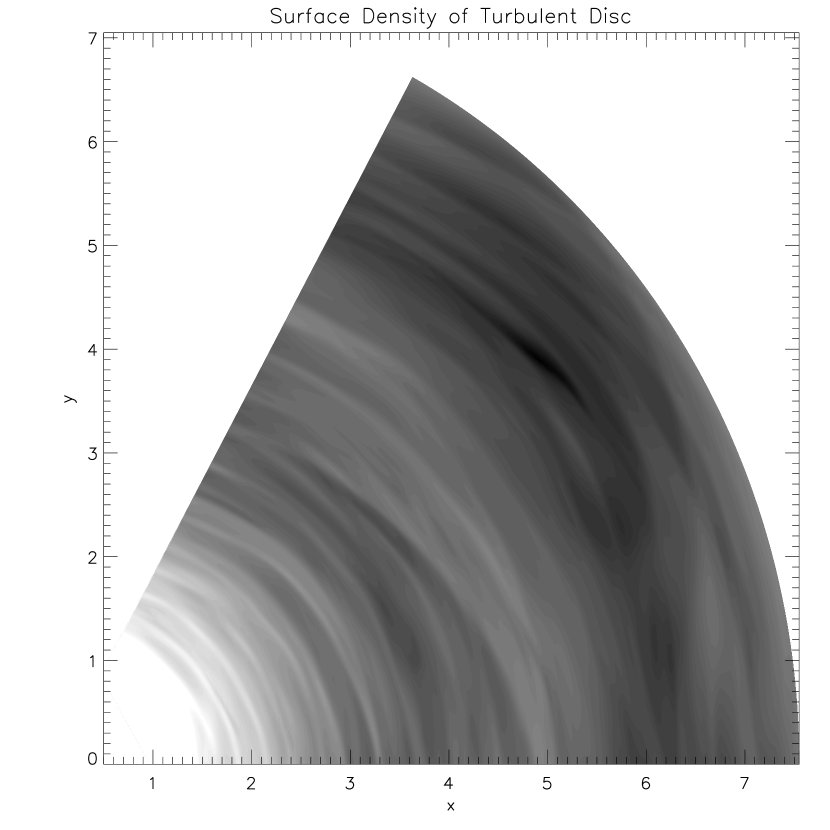
Figure 22: This plot shows the variations in density at the vertical midplane the disc model E.

Figure 23: This plot shows the radial variation of the azimuthally averaged density at the vertical midplane of the disc model E. The solid line corresponds to time $t=3825.5$, whereas the dashed line shows the initial values at $t=0$.

A greyscale plot of the density at the vertical midplane of the disc is shown in figure 22 corresponding to a time $t=3825.5$. The usual trailing waves generated by the turbulence can clearly be seen in this figure. The variation of the azimuthally averaged midplane density as a function of radius is plotted in figure 23. The solid line corresponds to the density distribution at time $t=3825.5$, whereas the dashed line shows the initial values at $t=0$. It is clear from this figure that some inward mass accretion has occurred.

4 Discussion

We have presented a study of cylindrical disc models in which a central domain in Keplerian rotation is unstable to the MRI. Models of varying disc size and aspect ratio $H/r$ were considered. They were initiated with small scale magnetic fields with zero net flux. Conservation of poloidal and toroidal flux ensures that this situation is maintained throughout the simulations. Input of flux through the boundaries which remain magnetically inactive does not occur. The models all attain a turbulent state, with statistical properties that do not depend on the initial conditions which is expected for genuine dynamo action.

As these models have been prepared for studies of disc– protoplanet interaction we have focused on relating the properties of the turbulent models to classical viscous disc theory [Shakura & Sunyaev (1973)]. This is an important issue, because besides providing a conceptual framework for disc studies, as emphasized by Balbus & Papaloizou (1999) it is still the main contact between disc theory and observations.

All models were found to attain a turbulent state with volume averaged stress parameter $\alpha\sim 5\times 10^{-3}$ and mean $\beta^{-1}\sim 0.01.$ We also found that the same results were obtained in a rotating frame and in agreement with Hawley (2000) they were independent of the extent of the azimuthal domain when this exceeded $\pi/3.$

The vertically and azimuthally averaged stress parameter showed large radial fluctuations. Time averaging for a period exceeding $3$ orbital periods was found to significantly reduce them. For models with $H/r=0.1$ stable variations with radius of a factor of two were then noted whereas for models with $H/r=0.2$ less variation was seen. Variations in the time averaged quantities are most probably due to some memory of initial conditions which take up to a viscous time to eradicate, this being shorter for the thicker disc models. The higher resolution thicker disc model tended to have larger values of $\alpha$ than a lower resolution counterpart, which may reflect a residual dependence on resolution (see Brandenburg et al. 1996).

The vertically and azimuthally averaged radial velocity showed large radial and temporal fluctuations of up to two orders of magnitude larger than the inflow velocity expected from classical viscous disc theory (see also SP). Time averaging for a period of at least $7-8$ orbital periods at the outer boundary of the Keplerian domain was required to reveal values of a magnitude comparable to the expected viscous inflow velocity. Comparison with the value derived from the averaged stress using viscous disc theory yielded schematic agreement for feasible averaging times. It is likely that very long averaging times are needed to eliminate residual fluctuations in the mean radial velocity and that such an averaging operation may only be possible for a very quiet and thin disc that has relaxed to a long term statistical steady state.

The behaviour described above must be borne in mind when considering laminar disc simulations with anomalous Navier–Stokes viscosity [e.g. Bryden et al (1999); Kley (1999); Lubow, Seibert & Artymowicz (1999); D’Angelo et al (2002)]. There, radial inflow velocities produced by the viscosity produce phenomena like mass flow through gaps when a protoplanet is embedded in a disc, due to the viscosity acting as a constantly acting source of friction. From the above discussion we might expect different dynamical behaviour in the gap region induced by a protoplanet in a genuinely turbulent disc (see paper II), where the instantaneous velocity fluctuations are much larger than the time averaged radial velocities arising from the turbulence–induced angular momentum transport. More generally the classical viscous disc theory cannot apply to a disc undergoing rapid changes due to external perturbation. It can only be used to describe the parts of the disc that are in a quasi-steady condition for long enough for appropriate averaging to be carried out.

4.1 Acknowledgments

We acknowledge John Hawley, Steve Balbus, Adriane Steinacker, and Caroline Terquem for useful discussions. The computations reported here were performed using the UK Astrophysical Fluids Facility (UKAFF) and the GRAND consortium supercomputing facility.

References

- [] Balbus, S. A., Hawley, J. F., 1991, ApJ, 376, 214
- [] Balbus, S. A., Papaloizou, J. C. B., 1999, ApJ, 521, 650
- [] Brandenburg, A., Nordlund, Å., Stein, R. F., Torkelsson, U., 1996, ApJ, 458, L45
- [] Brandenburg, A., 1998, in Theory of Black Hole Accretion Discs, eds. M.A. Abramowicz, G. Bjornsson, J.E. Pringle, CUP.
- [] Bryden, G., Chen, X., Lin, D. N. C., Nelson, R. P., Papaloizou, J. C. B., 1999, ApJ, 514, 344
- [] D’Angelo, G.; Henning, T.; Kley, W., 2002, A&A, 385, 647
- [] Fleming, T. P., Stone, J. M., Hawley, J. F., 2000, ApJ 530, 464
- [] Hawley, J. F., Stone, J. M., 1995, Computer Physics Communications, 89, 127
- [] Hawley, J. F., Gammie, C. F., Balbus, S. A., 1996, ApJ, 464, 690
- [] Hawley, J. F., 2000, ApJ, 528, 462
- [] Hawley, J. F., 2001, ApJ, 554, 534
- [] Kley, W., 1999, MNRAS, 303, 696
- [] Lin, D.N.C., Papaloizou, J.C.B., 1986, ApJ, 309, 846
- [] Lin, D.N.C., Papaloizou, J.C.B., 1993, Protostars and Planets III, p. 749-835
- [] Lubow, S.H., Seibert, M., Artymowicz, P., 1999, ApJ, 526, 1001
- [] Marcy, G. W., Cochran, W. D., Mayor, M., 2000, Protostars and Planets IV (Book - Tucson: University of Arizona Press; eds Mannings, V., Boss, A.P., Russell, S. S.), p. 1285
- [] Mayor, M., Queloz, D., 1995, Nature, 378, 355
- [] Nelson, R.P., Papaloizou, J.C.B., 2002, MNRAS, submitted (Paper II)
- [] Nelson, R. P., Papaloizou, J. C. B., Masset, F., Kley, W., 2000, MNRAS, 318, 18
- [] Papaloizou, J.C.B, Lin, D.N.C., 1984, ApJ, 285, 818
- [] Shakura, N. I., Sunyaev, R. A., 1973, A&A, 24, 337
- [] Steinacker, A., Papaloizou, J.C.B., 2002, ApJ, 571, 413
- [1977] Van Leer, B., 1977, J. Comp. Phys., 23, 276
- [] Vogt, S. S., Butler, R. P., Marcy, G. W.; Fischer, D. A.; Pourbaix, D., Apps, K., Laughlin, G., 2002, ApJ, 568, 352
- [] Ziegler, U., Rüdiger, G., 2000, A&A, 356, 1141
- []