On the Eccentricity Distribution of Coalescing Black Hole Binaries Driven by the Kozai Mechanism in Globular Clusters

Abstract

In a globular cluster, hierarchical triple black hole systems can be produced through binary-binary interaction. It has been proposed recently that the Kozai mechanism could drive the inner binary of the triple system to merge before it is interrupted by interactions with other field stars. We investigate qualitatively and numerically the evolution of the eccentricities in these binaries under gravitational radiation (GR) reaction. We predict that $\sim 30$% of the systems will possess eccentricities $>0.1$ when their emitted gravitational waves pass through 10 Hz frequency. The implications for gravitational wave detection, especially the relevance to data analyses for broad-band laser-interferometer gravitational wave detectors, are discussed.

1 Introduction

Globular clusters are excellent birthplaces for black hole (BH) binaries. In our Galaxy, a globular cluster (GC) contains typically $N=10^{6}$ stars and resides normally in the galactic halo. Typical ages of these clusters are estimated to be 12 billion years, and the clusters contain the oldest stars known in our Galaxy. Stellar evolution theory predicts that massive stars with mass above 10 $M_{\odot}$ would evolve into black holes or neutron stars in $\sim 10^{7}$ years. For a typical GC that follows the initial mass function (IMF) given by Scalo (1986), a significant number of BHs ($\sim 6\times 10^{-4}N$ for initial masses $>20$–25$M_{\odot}$) should have been born. These BHs would be the most massive stars in the cluster, and hence dynamical two-body relaxation causes them to sink rapidly towards the core. In the core, BH binaries are expected to form. The single BHs form binaries preferentially with another BH, and BHs born in binaries with a lower mass stellar component rapidly exchange the companion for another BH through three body relaxation processes. If these BH binaries merge within the Hubble time, they would become excellent sources for upcoming gravitational wave (GW) detectors (e.g. Thorne (1987)).

It has been argued that globular clusters are unlikely places to harbor BH mergers (or subsequently to harbor a massive central black hole) if we consider binary-single interactions alone (e.g. Portegies Zwart & McMillan (2000)). Numerical simulations show that binary-single interactions tend to throw out these BH binaries and only 8% of BHs will be retained in the GC within its lifetime. Miller & Hamilton (2002) argued that this picture will be different if we consider binary-binary interactions. A substantial fraction of hierarchical triple BH systems can result from binary-binary interactions. The well-known Kozai mechanism (Kozai (1962)) can then drive the inner binaries of a significant fraction of these triples to extreme eccentricities and thus reduce their time to coalescence to be shorter than the Hubble time. This is because the coalescence time scale $\tau_{\rm GR}$ due to gravitational radiation for a binary with fixed semi-major axis $a$ has a strong dependence on the eccentricity $e$ through the quantity $\epsilon=1-e^{2}$ (Peters (1964)),

$$\tau_{\rm GR}\approx 6\times 10^{10}\frac{(a/{\rm AU})^{4}(\epsilon/0.01)^{3.5}}{(m_{0}+m_{1})m_{0}m_{1}/\mbox{$M_{\odot}$}^{3}}\ \ \ \mbox{yr},$$ (1)

where $m_{0}$ and $m_{1}$ are the masses of each binary component. In their paper, Miller & Hamilton (2002) have compared the coalescence time scale with the time scale for the system to be disrupted by interactions with field stars. They concluded that in a substantial fraction of cases, the system will achieve extreme eccentricities ($\epsilon\sim 0$) and will merge by gravitational radiation before the disruption. The BH mergers may thus be retained in the GCs and a central intermediate-mass BH may form through subsequent mergers.

We are motivated by the fact that the proposed mechanism promises stellar mass BH-BH mergers with extremely high initial eccentricities and that they are potential sources for upcoming gravitational wave detectors such as LIGO. We investigate in this paper whether or not these systems would still possess finite eccentricities when the emitted gravitational waves enter LIGO’s frequency band. The eccentricities of these sources are particularly interesting as no astrophysical merger sources were expected before to possess significant eccentricities when they reach the LIGO band. Current efforts in detecting GWs from coalescing BH binary sources thus focus on waves from circular orbits (see Buonanno, Chen, & Vallisneri (2002) for recent development). On the other hand, it is well-known that the gravitational waveform of an eccentric binary could be significantly different from that of a circular one and different detection strategies are required for optimal detections (e.g., Peters & Mathews (1963); Peters (1964); Lincoln & Will (1990); Moreno-Garrido, Mediavilla, & Buitrago (1995); Gopakumar & Iyer (2002); Glampedakis, Hughes, & Kennefick (2002)). Our work can thus help shed light on the importance of the eccentricities for detecting GWs from these sources.

In this paper, we investigate in detail the eccentricity evolution of these merger systems under the impact of gravitational radiation reaction (simplified as the GR effect). This is in addition to the Kozai mechanism and the post-Newtonian periastron precession (simplified as the PN effect) considered by previous authors. It has been long realized (Peters & Mathews (1963); Peters (1964)) that gravitational radiation reaction is very efficient in circularizing coalescing binaries. For the systems we are considering, this circularization effect would have to compete with the “eccentricity enhancing” Kozai mechanism. Under the Kozai mechanism and the PN effect, the system tries to maintain secular cyclic eccentricity oscillations at fixed amplitude (with exceptions at critical inclination angles, see text). The GR effect operates most efficiently near the minimum $\epsilon$ of each cycle. In some cases, it could drive a system near its minimum $\epsilon$ directly towards merger. In other cases, it would affect the minimum $\epsilon$ and alter the otherwise fairly strict periodic evolution trajectory of the system. In particular, it will enhance rapidly the importance of the PN effect which in turn would introduce fast oscillations to destroy the Kozai resonance. The Kozai resonance will eventually be quenched either directly by the GR effect, or by the PN effect before the GR effect takes over. We will discuss the details of these effects and their implications for the evolution of the eccentricities and gravitational wave frequencies.

In section 2, we give a summary of the relevant features of the Kozai mechanism and derive an explicit general expression for the minimum $\epsilon$ (or maximum eccentricity) the system can reach for arbitrary values of BH masses and initial eccentricities. In section 3, we discuss the evolution of the system parameters under gravitational radiation reaction (the GR effect). The equations of motion are described in subsection 3.1. We describe technical details to estimate the minimum $\epsilon$ the system can reach in subsection 3.2. The PN effect and its role in determining the evolution of the gravitational wave frequency are described in subsection 3.3. A procedure to obtain the relation of the gravitational wave frequencies and the eccentricity at various evolution stages is given in subsection 3.4. Two numerical examples are presented in subsection 3.5. In section 4, we estimate the eccentricity distribution when the gravitational waves enters the LIGO band. Our results are then summarized in section 5.

2 Kozai Mechanism

2.1 Principle and Notation

The Kozai Mechanism was initially proposed (Kozai (1962)) to describe the perturbation of asteroids due to Jupiter. This mechanism describes the secular evolution of the orbit of a hierarchical triple system as a result of cyclic exchange of angular momentum between the inner binary and orbit of the distant tertiary. One of the most interesting results of the Kozai mechanism is that the eccentricity of the inner binary can reach very large values while the semi-major axis remains unchanged, provided that the initial mutual inclination angle of the two binaries reaches a certain critical value. Although the mechanism was proposed for a system where the mass of one component in the inner binary is much smaller than those of the others, the mechanism has then been found to operate in hierarchical triple systems with arbitrary masses (Lidov & Ziglin (1976)).

A hierarchical triple star system consists of a close binary of masses $m_{0}$, $m_{1}$, and a tertiary $m_{2}$ in a much wider outer orbit (Fig. 1). The dynamics of the system can be treated as if it consists of an inner binary of point masses $m_{0}$ and $m_{1}$, and an outer binary of point masses $m_{2}$ and $M_{1}=m_{0}+m_{1}$. The separations of the masses each binary are denoted $r_{1}$ and $r_{2}$. The mutual inclination angle of the two binaries is denoted $I$. For the inner and outer binaries respectively, we denote the eccentricities $e_{1}$ and $e_{2}$, reduced masses $\mu_{1}=m_{0}m_{1}/M_{1},\mu_{2}=m_{2}M_{1}/(M_{1}+m_{2})$, semimajor axes $a_{1}$ and $a_{2}$. We define $g_{1}$ as the argument of pericenter of the inner binary relative to the line of the descending node.

Throughout this paper, we frequently use quantities $\epsilon=1-e^{2}_{1}$ and $b_{2}=a_{2}\sqrt{1-e^{2}_{2}}$ to simplify our discussion. Angular momentum is normalized to have dimension $\sqrt{\mbox{Length}}$ by dividing by the quantity $L_{1}=\mu_{1}\sqrt{GM_{1}}$. We use notation $\alpha_{0}$, $\beta_{0}$, and $\gamma$ for the normalized magnitude of total angular momentum of the triple system, of the outer binary, and of the inner binary respectively. Our $\alpha_{0}$ and $\beta_{0}$ are related to dimensionless quantities $\alpha$ and $\beta$ used in previous literature by $\alpha=\alpha_{0}/\sqrt{a_{1}}$, and $\beta=\beta_{0}/\sqrt{a_{1}}$. It follows that $\gamma=\sqrt{a_{1}\epsilon}$, $\beta_{0}=\mu_{2}/\mu_{1}\sqrt{M_{2}a_{2}/{M_{1}}(1-e^{2}_{2})}$, and that $\alpha_{0}$ is related to $\beta_{0}$ and $a_{1}\epsilon$ through the following trigonometric relation

$$\cos I=\frac{\alpha^{2}_{0}-\beta^{2}_{0}-a_{1}\epsilon}{2\beta_{0}\sqrt{a_{1}\epsilon}}.$$ (2)

As we shall see, during the binary’s Kozai mechanism-induced evolution, $\alpha_{0}$, $\beta_{0}$, and $a_{1}$ are conserved while $\epsilon$ changes. It follows that $\alpha_{0}=\beta_{0}$ is the critical condition for the system to be able to evolve to $\epsilon=0$ ($e_{1}=1$). This implies a critical initial $I$ of

$$I_{0}=I_{c}=\cos^{-1}\left(-\frac{\sqrt{\epsilon_{0}}}{2\beta}\right),$$ (3)

where $\epsilon_{0}$ is the initial $\epsilon$. For this solution to exist, $\beta\geq\sqrt{\epsilon_{0}}/2$ is required.

The total Hamiltonian of the system can be written as $H=H_{1}+H_{2}+H^{{}^{\prime}}$, where $H_{1}$ and $H_{2}$ are the Hamiltonians for the inner and outer binaries respectively as if they were isolated binaries of point masses. $H^{{}^{\prime}}$ is the perturbative Hamiltonian which includes perturbation of the inner binary by the presence of the tertiary $m_{2}$ and perturbation of the outer binary by the finite size of the binary component $M_{1}$. For $r_{1}/r_{2}\ll 1$ and $(m_{2}/M_{1})(r_{1}/r_{2})^{3}\ll 1$, the Hamiltonian $H^{{}^{\prime}}$ can be expanded in powers of $r_{1}/r_{2}$. The first non-zero contribution comes from the term of order $(r_{1}/r_{2})^{2}$, labeled as quadrupole term because of the degree of the Legendre polynomial associated with it. This term is sufficient for our discussion as we are only concerned about cases with large initial mutual inclination angle $I_{0}$ (see Ford, Kozinsky, & Rasio 2000 for discussions concerning the octupole terms of order $(r_{1}/r_{2})^{3}$).

It is this perturbative Hamiltonian $H^{{}^{\prime}}$ that leads to a secular evolution of the triple system. In the first approximation, the secular evolution can be described by $H^{{}^{\prime}}$ doubly-averaged over the mean anomaly of both the inner and the outer orbits. It turns out that the doubly-averaged $H^{{}^{\prime}}$, the total angular momentum of the system ($\alpha_{0}$), the energy of each binary (or equivalently $a_{1}$ and $a_{2}$), and the magnitude of the angular momentum of the outer binary ($\beta_{0}$, or equivalently $e_{2}$) are conserved quantities. The secular evolution of the triple system can therefore be fully described in terms of time-evolving $\epsilon$ and $g_{1}$. A useful constant of integration can be derived from equation (2),

$$a_{1}\epsilon\left(\cos I+\frac{\sqrt{\epsilon}}{2\beta}\right)^{2}=\frac{(\alpha^{2}_{0}-\beta^{2}_{0})^{2}}{4\beta^{2}_{0}}.$$ (4)

Note that the quantity on the left hand side is conserved as long as the total angular momentum ($\alpha_{0}$) and that of the outer binary ($\beta_{0}$) are conserved. Also, whenever $\sqrt{\epsilon}\ll 2\beta$, $a_{1}\epsilon\cos^{2}I$ is a constant.

The secular evolution is a result of coherent additions of perturbations from the tertiary to the inner binary. Therefore, any mechanism that perturbs the phase relation of the system could modify the evolution of $\epsilon$ and $g_{1}$. For black hole systems, an important effect comes from the general relativistic periastron precession of the inner binary. Inclusion of this effect can be found in Miller & Hamilton (2002) and Blaes, Lee & Socrates (2002). In summary, contribution of the periastron precession in the first-order post-Newtonian approximation can be added to the doubly-averaged Hamiltonian as $\it{H}_{\rm PN}=-k\theta_{\rm PN}/\sqrt{\epsilon}$, where,

$$\theta_{\rm PN}=8\times 10^{-8}\frac{(M_{1}/\mbox{$M_{\odot}$})^{2}}{m_{2}/\mbox{$M_{\odot}$}}\left(\frac{b_{2}}{a_{1}}\right)^{3}\frac{1}{a_{1}/{\rm AU}},$$ (5)

and $k=3Gm_{0}m_{1}m_{2}a^{2}_{1}/(8M_{1}b^{3}_{2})$ is a quantity related to the evolution time scale. Apparently the influence of the periastron precession (abbreviated as PN effect) is the largest (in the sense that $\theta_{\rm PN}$ is the largest) for systems consisting of a tight and massive inner binary and a light, far-out third component. With the addition of this PN effect, the total Hamiltonian remains conserved. It can be written as $H=kW$ (Miller & Hamilton (2002)), where

$$W(\epsilon,g_{1})=-2\epsilon+\epsilon\cos^{2}I+5(1-\epsilon)\sin^{2}g_{1}(\cos^{2}I-1)+\theta_{\rm PN}/\epsilon^{1/2},$$ (6)

is a conserved quantity.

2.2 Eccentricity Evolution in Absence of the GR Effect

The trajectory of $e_{1}$ and $g_{1}$ in the phase space are known to be determined by the values of $\alpha$ and $\beta$ for given initial system parameters (Lidov & Ziglin (1976)). In the general case of initial $e_{1}\neq 0$,$1$ and in the absence of the GR effect, the quantities $e_{1}$, $g_{1}$ undergo cyclic oscillations. A necessary condition for a large change in $e_{1}$ is that $I_{0}>\cos^{-1}\sqrt{3/5}\sim 39^{o}$ for a restricted case where $m_{0}\ll m_{2}\ll m_{1}$. This condition still holds for arbitrary masses when the PN effect is weak (as can be proved using eq. [8]). The time scale for the system to swing from $e_{1}\sim 0$ to $e_{1}\sim 1$ is estimated to be (Innanen, Zheng, Mikkola, & Valtonen (1997)),

$$\tau_{\rm{evol}}\approx 0.16f\left(\frac{M_{1}}{m_{2}}\right)^{1/2}\left(\frac{a_{2}}{a_{1}}\right)^{3/2}\frac{(a_{2}/{\rm AU})^{3/2}}{(m_{2}/\mbox{$M_{\odot}$})^{1/2}}(1-e^{2}_{2})^{3/2}\ \rm{yr},$$ (7)

where $f\sim 0.42\log(1/{e_{1}}_{0})/\sqrt{(\sin^{2}(I_{0})-0.4}$ is a quantity of magnitude a few, ${e_{1}}_{0}$ is the initial value of $e_{1}$, and $I_{0}$ is the initial value of $I$. This time scale should be much longer than the orbital periods of both binaries because it is an orbital averaged effect.

The minimum value of $\epsilon$ (denoted $\epsilon_{\rm min}$) for arbitrary masses $m_{0}$, $m_{1}$, $m_{2}$, and arbitrary $\epsilon_{0}$ can be solved for using the fact that the Hamiltonian is conserved, that is, $W(\epsilon_{0},g_{0})=W(\epsilon_{\rm min},g_{m})$ (eq. [6]). We are interested the cases $\epsilon_{\rm min}$ $\sim 0$ and $\epsilon_{\rm min}$$\ll\epsilon_{0}$. It follows that $g_{m}=\pi/2$ for $I_{0}\neq I_{c}$ (Lidov & Ziglin (1976)), $\epsilon^{4}_{\rm min}\ll\epsilon^{2}_{\rm min}$, and $\epsilon_{\rm min}\ll 2\beta$. The assumption that $\epsilon_{\rm min}\ll 2\beta$ is valid as long as there exists a solution for the critical initial value $\cos I_{c}=-\sqrt{\epsilon_{0}}/(2\beta)$. Under these conditions, the $\cos^{2}I$ term in $W(\epsilon_{\rm min},g_{m})$ can be rewritten in terms of $\cos^{2}I_{0}$ and $\epsilon_{\rm min}$. An explicit approximation formula for $\epsilon_{\rm min}$ is then obtained by solving the resulting quadratic equation as

$$\epsilon^{1/2}_{\rm min}\approx\frac{1}{2\Omega}\left\{\theta_{\rm PN}+\sqrt{\theta^{2}_{\rm PN}+20\Omega\epsilon_{0}\left[\cos I_{0}+\sqrt{\epsilon_{0}}/(2\beta)\right]^{2}}\right\}.$$ (8)

By using equation (4), we have

$$\epsilon^{1/2}_{\rm min}\approx\frac{1}{2\Omega}\left[\theta_{\rm PN}+\sqrt{\theta^{2}_{\rm PN}+5\frac{\Omega}{a_{1}}\frac{(\alpha^{2}_{0}-\beta^{2}_{0})^{2}}{\beta^{2}_{0}}}\right].$$ (9)

Here

$$\Omega=5-2\epsilon_{0}+\epsilon_{0}\cos^{2}I_{0}+\frac{\theta_{\rm PN}}{\sqrt{\epsilon_{0}}}+4\epsilon_{0}(\cos I_{0}+\frac{\sqrt{\epsilon_{0}}}{2\beta})^{2}+5(1-\epsilon_{0})(\cos^{2}I_{0}-1)\sin^{2}(g_{0}).$$ (10)

For the restricted case of $m_{0}\ll m_{2}\ll m_{1}$, we have $\beta\rightarrow\infty$, $I_{c}\rightarrow 90^{o}$. We recover equation (8) of Miller & Hamilton (2002) using their assumptions that $\epsilon_{0}\approx 1$, $\theta_{\rm PN}\ll 3$ and $5\cos^{2}I_{0}\ll 3$. We then also recover the classical limit $e_{\rm max}=\sqrt{1-\epsilon_{\rm min}}=\sqrt{1-(5/3)\cos^{2}I_{0}}$ (e.g., Innanen et al. 1997) by setting $\theta_{\rm PN}=0$.

It follows from equation (8) that a condition for achieving extremely small $\epsilon_{\rm min}$ is $\theta_{\rm PN}\ll 1$ and $I_{0}\approx I_{c}>90^{o}$, which corresponds to $\alpha\approx\beta$ (eq.[4]). Note that $I_{c}>90^{o}$ means that the outer binary should initially be in a retrograde orbit with the inner one. This is consistent with what we obtained in the classical limit ($\theta_{\rm PN}=0$), where a system can evolve to $e=1$ starting from any initial eccentricity if $\alpha=\beta$ (or $I_{0}=I_{c}$) (see details in Lidov & Ziglin (1976)). The critical values of $I_{0}$ above which the system can have a significant change in $\epsilon$ can also be derived. If we demand $\epsilon_{\rm min}\leq 0.5\epsilon_{0}$, we would obtain from equation (8) $\cos^{2}I_{0}\leq 3/5$, or $I_{0}\geq 39^{o}$ for $\epsilon_{0}\sim 1$ and $\theta_{\rm PN}\sim 0$. This is the same as the known classical limit for the restricted problem.

Two important constants can be derived from equation (8) for triple systems with arbitrary masses but negligible PN effect. As $\theta_{\rm PN}\rightarrow 0$, $\Omega$ is a constant $\sim 3$ for $\epsilon_{0}\approx 1$ and $I_{0}\sim I_{c}$,

$$a_{1}\epsilon_{\rm min}\approx\frac{5}{12}\frac{(\alpha^{2}_{0}-\beta^{2}_{0})^{2}}{\beta^{2}_{0}}.$$ (11)

It thus follows from equation (4) that the mutual inclination angle at $\epsilon_{\rm min}$  (denoted $I_{m}$) satisfies

$$\cos^{2}I_{m}\approx 3/5,$$ (12)

for $\sqrt{\epsilon_{\rm min}}\ll 2\beta$.

3 Influence of Gravitational Radiation Reaction (GR Effect)

In this section, we discuss how the GR effect damps the Kozai oscillations and eventually leads to the merger of the system. As the gravitational radiation frequency depends directly on the quantity $a_{1}\epsilon$ ($\gamma^{2}$, or the semi-latus rectum) (section 4, eq. [37]), we focus our discussions on the evolution of this quantity. We first discuss the equations that govern the evolution of the system where the GR effect is included. We then derive the minimal $\epsilon$ ($\epsilon_{\rm min}$) obtained at the first Kozai cycle and then determine the evolution of $\epsilon_{\rm min}$ during subsequent cycles, depending on the roles of the PN effect and the GR effect. The evolution of the frequency of the gravitational wave emitted by the inner binary can then be determined.

3.1 Equations of Motion

The presence of gravitational radiation has important impacts on the eccentricity evolution of the inner binary. First, the radiation carries away energy and angular momentum and tends to shrink and circularize the orbit. The decay of the orbit subsequently changes the values of $\alpha$ and $\beta$ and thus modifies the secular evolution trajectory of the system. In particular, the effect of periastron precession becomes stronger rapidly with the decay of the orbit (see eq. [5]). This results in rapid oscillations of $g_{1}$ that could destroy the secular oscillation of $\epsilon$. As for the outer binary, the orbit remains much wider than the inner one, so its energy (equivalently $a_{2}$) and magnitude of angular momentum ($\beta_{0}$, or equivalently $e_{2}$) can therefore still be treated as conserved quantities.

The GR effect is the strongest at $\epsilon\sim\epsilon_{\rm min}$ within each Kozai cycle because of the strong dependence of the merger time scale $\tau_{\rm GR}$ on $\epsilon$ (eq. [1]). When the PN effect is negligible and the GR effect does not affect the Kozai cycles dramatically, we have $a_{1}\propto\epsilon^{-1}_{\rm min}$ according to equation (11). The evolution of the parameters $\theta_{PN}$, $\tau_{\rm evol}$, and $\tau_{\rm GR}$ with the decay of the orbit can then be summarized as follows.

$$\theta_{\rm PN}\propto a^{-4}_{1}\propto\epsilon^{4}_{\rm min}$$ (13)

$$\tau_{\rm evol}\propto a^{-3/2}_{1}\propto\epsilon^{3/2}_{\rm min}$$ (14)

$$\tau_{GR}\propto a^{4}_{1}\epsilon^{7/2}_{\rm min}\propto\epsilon^{-0.5}_{\rm min}.$$ (15)

It is apparent that, as the orbit of the inner binary shrinks and circularizes, the value of $\tau_{GR}$ decreases proportional to $\epsilon^{-0.5}_{\rm min}$ while the time the system spends at $\epsilon_{\rm min}$ ($\tau^{{}^{\prime}}_{\rm evol}=\tau_{\rm evol}\sqrt{\epsilon_{\rm min}}$) increases proportional to $\sim\epsilon_{\rm min}^{2}$. When $\tau_{\rm GR}$ becomes of order $\tau_{\rm evol}\sqrt{\epsilon_{\rm min}}$, the gravitational merger will take place within one Kozai cycle near $\epsilon\sim\$$\epsilon_{\rm min}$.

The evolution of the system can be calculated through a set of hybrid equations that combines the equations of motion derived from the conserved Hamiltonian $W(\epsilon,g_{1})$ (Lidov 1976, eq. [32]–[33]) including the PN effect and that from quadrupole gravitational radiation (Peters (1964), eq. [5.6]–[5.7]). These are the same equations used in Blaes, Lee, & Socrates (2002). The evolution equations govern the four parameters $\epsilon$, $g_{1}$, $a_{1}$, and $\alpha_{0}$ and are given by

$$\frac{d\epsilon}{dt} = -10\kappa_{E}a^{1.5}_{1}\sqrt{\epsilon}(1-\epsilon)(1-\cos^{2}I)\sin(2g_{1})+\frac{\kappa_{G}}{a_{1}^{4}}\frac{1-\epsilon}{\epsilon^{2.5}}(\frac{425}{304}-\frac{121}{304}\epsilon),$$ (16)

$$\frac{dg_{1}}{dt} = \kappa_{E}a^{1.5}_{1}\left\{\frac{1}{\sqrt{\epsilon}}\left[4\cos^{2}I+(5\cos 2g_{1}-1)(\epsilon-\cos^{2}I)\right]\right.$$ (17)

$$\mbox{}\left.+\frac{\cos I}{\beta}\left[2+(1-\epsilon)(3-5\cos 2g_{1})\right]+\frac{\theta_{\rm PN}}{\epsilon}\right\},$$

$$\frac{da_{1}}{dt} = -\frac{6}{19}\frac{\kappa_{G}}{a^{3}_{1}}\frac{1}{\epsilon^{3.5}}(\frac{425}{96}-\frac{61}{16}\epsilon+\frac{37}{96}\epsilon^{2}),$$ (18)

$$\frac{d\alpha_{0}}{dt} = -\frac{3}{19}\frac{\kappa_{G}}{a^{3.5}_{1}}\frac{1}{\epsilon^{2}}(\frac{15}{8}-\frac{7}{8}\epsilon)\frac{\sqrt{a_{1}\epsilon}+\beta_{0}\cos^{2}I}{\alpha_{0}},$$ (19)

where $\theta_{\rm PN}$ is defined in equation (5), and

$$\kappa_{\rm E} = 7.4554\times 10^{-8}(\frac{m_{2}}{M_{1}})^{0.5}\frac{(m_{2}/\mbox{$M_{\odot}$})^{0.5}}{(a_{2}/{\rm AU})^{3}(1-e^{2}_{2})^{1.5}}\frac{1}{{\rm AU}^{1.5}},$$ (20)

$$\kappa_{\rm G} = 7.8218\times 10^{-26}\frac{m_{0}m_{1}M_{1}}{\mbox{$M_{\odot}$}^{3}}{\rm AU}^{4}.$$ (21)

The evolution of the angular momentum $\gamma$ can be written as (see eq. [16],[18]),

$$\frac{d\gamma}{dt}=-5\kappa_{E}a^{2}_{1}\sin^{2}I\sin 2g_{1}-\frac{3}{19}\kappa_{G}a^{-3.5}_{1}\epsilon^{-2}(\frac{15}{8}-\frac{7}{8}\epsilon^{2}).$$ (22)

Equations (16)–(19) provide a valid description of the evolution as long as the energy ($a_{1}$) is approximately conserved within each cycle, and as the total angular momentum vector of the triple system is conserved. These are necessary conditions for the validity of the equations derived from the conserved Hamiltonian and the following considerations justify them for the systems that interest us.

We have assumed that the triple systems in globular clusters consist of stellar mass BHs with initial orbital separations on the order of AU, and moderate initial $\epsilon\sim 1$ (see the discussion of parameters in section 4 below). The systems are required to obtain extremely small $\epsilon_{\rm min}$$\sim 0$ during their secular evolution in order to merge well before the system is disrupted by interactions with field stars (Miller & Hamilton (2002)). Equation (16) and (17) indicate that at each Kozai cycle, such systems would spend most of their time at moderate $\epsilon\sim 1$, and a very small fraction of the time ($\propto\sqrt{\epsilon_{\rm min}}$) at extremely small values (see also Innanen, et al. 1997). Note that gravitational radiation reaction is negligible at moderate $\epsilon$ and $a_{1}$ as $\kappa_{G}\ll\kappa_{E}$ (eq. [20],[21]) for such systems. The energy (equivalently $a_{1}$) can thus be treated approximately as conserved for most of the cycles (see also eq. [18]).

The total angular momentum vector can also be treated as conserved within each cycle as long as $\epsilon_{\rm min}$$\sim 0$. It is known that, for an isolated system under gravitational radiation reaction, the angular momentum loss is negligible ($\propto\kappa_{G}\epsilon^{1.5}_{\rm min}$) at $\epsilon_{\rm min}$$\sim 0$ (eq. [22], second term). Moreover, gravitational radiation reaction will not change the direction of the angular momentum of the inner system. It is thus conceivable that as long as $\epsilon_{\rm min}$$\sim 0$, the evolution of the angular momentum of the inner binary ($\gamma$) is negligibly affected by the GR effect, and the vector of the total angular momentum can be treated as conserved throughout the cycles. For our systems, the GR effect starts to dominate at $\epsilon_{\rm min}$$\sim 0$ because of the extremely small $\epsilon_{\rm min}$ required for the system to merge before the system is disrupted by a field star. These justify the validity of equations (16)–(19).

3.2 Estimation of $\epsilon_{\rm min}$

The minimum value of $\epsilon$ that a system can reach within its first Kozai cycle (denoted $\epsilon_{\rm min}$) is best estimated using equation (16). At $\epsilon=\epsilon_{\rm min}$, $d\epsilon/dt=0$, we obtain,

$$\sin^{2}g_{m}=\frac{1+\sqrt{1-(\gamma_{0}\epsilon^{-3}_{\rm min}a^{-5.5}_{1}\sin^{-2}I_{m})^{2}}}{2},$$ (23)

where

$$\gamma_{0}=\frac{425}{3040}\frac{\kappa_{G}}{\kappa_{E}}=1.467\times 10^{-19}\frac{\mbox{$M_{\odot}$}^{3}}{m_{0}m_{1}M_{1}}\left(\frac{M_{1}}{m_{2}}\right)^{1/2}\frac{(a_{2}/{\rm AU})^{3}(1-e^{2}_{2})^{3/2}}{(m_{2}/\mbox{$M_{\odot}$})^{1/2}}{\rm AU}^{5.5},$$ (24)

and where $\sin^{2}I_{m}$ is related to $\epsilon_{\rm min}$ through equation (2). We estimate $\epsilon_{\rm min}$ by assuming that $a_{1}$ is a constant and solving implicitly the equation

$$\Delta W=W(g_{0},\epsilon_{0})-W(g_{m},\epsilon_{\rm min})=0.$$ (25)

In our numerical work, we actually solve for $\epsilon_{\rm min}$  by minimizing $(\Delta W)^{2}$ using a downhill simplex method developed by Nelder and Mead (1965) (available in Matlab). This method has proved to be robust in finding local minima. However, because of the existence of multiple solutions to equation (25) (with at least one other solution $\epsilon=\epsilon_{0}$ and $g_{1}=g_{0}$), a good initial guess is essential for a well-converged solution.

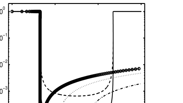
Figure 5: Phase diagram of $\epsilon$ vs $g_{1}$ for the same initial parameters as in Fig. 4 but with various $I_{0}$. We have $I_{0}=98^{o}$ (dashed line), $I_{0}=99.05^{o}$ (dotted line), $I_{0}=99.2^{o}$ (solid line with circles), $I_{0}=99.3^{o}$ (dash-dot line), $I_{0}=99.5^{o}$ (solid line). For general cases, $\epsilon_{\rm min}$ occurs at $g_{1}=g_{m}=90^{o}$. For $I_{0}\sim I_{c}$, $g_{m}$ is significantly deviated from $90^{o}$.

We made our initial guess $\epsilon_{\rm min}$  by considering the following two limits for $g_{m}$ based on equation (23). In the first limit, gravitational radiation reaction is weak, or $a^{11/2}_{1}\epsilon^{3}\gg\gamma_{0}$, we have $g_{m}\sim 90^{o}$. Equation (8) can then serve as a very good approximation to $\epsilon_{\rm min}$. In the second limit, gravitational radiation is very important, $g_{m}$ could deviate significantly from $90^{o}$. The extreme limit occurs around $I_{0}=I_{c}$ or $\alpha_{0}=\beta_{0}$ (eq. [4]). As with the critical case of $\alpha=\beta$ in the classical limit, a system starting with $\epsilon_{0}\sim 1$ will pass through an unstable stationary point $\epsilon\sim 1$ and $g_{1}\sim\sin^{-1}\sqrt{2/5}$ and move on towards a stationary (and stable in the classical limit) point $\epsilon\sim 0$, and $g_{c}=\sin^{-1}\left[1/(2\beta)\sqrt{(8\beta^{2}-1)/5}\right]$ (Lidov & Ziglin (1976), eq. [46]). If it were not for the GR effect, the system would reach $e_{1}=1$ at this stable point. With the presence of the GR effect, the angle $g_{1}$ will be steered away from this point while $\epsilon$ is steered away from a true zero value (see also Fig. 5). However, we expect the value of $g_{m}$ to be very close to $g_{c}$ (at $\epsilon_{\rm min}$$\sim 0$, $dg/dt\propto\epsilon_{\rm min}\sim 0$) (eq. [17], ignoring the PN effect). In this limit, the minimum $\epsilon$ can thus be estimated using $g_{m}\sim g_{c}$ and assuming constant $a_{1}$. Specifically, we again use the minimization program introduced previously to solve equation

$$a^{5.5}_{1}\epsilon^{3}_{\rm min}=\gamma_{0}\frac{1}{\sin^{2}I_{m}}\frac{1}{\sin 2g_{c}},$$ (26)

for $\epsilon_{\rm min}$, where $\sin^{2}I_{m}$ is related to $\epsilon_{\rm min}$  by equation (2).

Without knowing the solution ahead of time, we simply feed values of $\epsilon_{\rm min}$  estimated for these two limits as initial guesses to the minimization program and then select the solutions of $(\Delta W)^{2}=0$ with minimum residues. In all cases, the residues of the minimization are monitored to ensure correct convergence.

3.3 PN effect

The importance of the PN effect increases rapidly with the decay of the orbit as $\theta_{\rm PN}\propto a^{-4}_{1}$. This effect has a direct impact on the oscillatory behavior of $g_{1}$ (eq. [17]), through which it can affect the evolution of $\epsilon$ and thus $a_{1}$$\epsilon_{\rm min}$  (eq. [16]). The importance of the PN effect to the evolution of $\epsilon$ and $a_{1}$$\epsilon_{\rm min}$, however, depends on the role of the GR effect.

The PN effect can be neglected if the GR effect dominates in the evolution of $\epsilon$ before the PN effect becomes important in the evolution of $g_{1}$. Once the GR effect dominates, the evolution of $\epsilon$ decouples from that of $g_{1}$ and the Kozai cycle is terminated. In the cases we are interested in, this transition occurs near $\epsilon_{\rm min}$$\sim 0$. When both the GR and the PN effects are not important, the quantity $a_{1}$$\epsilon_{\rm min}$  is roughly a constant (eq. [11]). After the GR effect dominates, it evolves according to equation (5.11) of Peters (1964) and remains a constant as long as $\epsilon_{\rm min}$$\sim 0$. The overall evolution of $a_{1}$$\epsilon_{\rm min}$  can therefore be conveniently described using Peters’ equation with $a_{1}$ and $\epsilon_{\rm min}$  of the first Kozai cycle (see section 3.2) as the initial data.

The PN effect has a significant impact on the evolution of $\epsilon$ and $a_{1}$$\epsilon_{\rm min}$ if it dominates in the evolution of $g_{1}$ before the GR effect becomes important. In this case, a dominating PN effect will introduce a fast oscillation in $g_{1}$ and thus in $\epsilon$ (eq. [17]) and will terminate the Kozai cycle. The GR effect will eventually dominate in the evolution of $\epsilon$ and Peters’ formula can again describe the evolution of $a_{1}$$\epsilon_{\rm min}$. However, when the PN effect is important, the quantity $a_{1}$$\epsilon_{\rm min}$ can no longer be approximated as a constant before the GR effect dominates. It will evolve to a larger value than that in the first Kozai cycle (see eq. [3.2]). The results based on Peters’ formula with initial values taken at the first Kozai cycle can therefore be used to set the lower bound on $a_{1}\epsilon_{\rm min}$.

An upper limit for the quantity $a_{1}$$\epsilon_{\rm min}$  when the PN effect is important can be set based on the following considerations. First, the fast oscillation induced by the PN effect will be damped away under the GR effect. In light of equation (9), the quantity $\Omega$ will evolve from a rough constant of 3–5 towards $\Omega\sim\theta_{\rm PN}/\sqrt{\epsilon_{0}}\rightarrow\infty$ as $\theta_{\rm PN}\rightarrow\infty$ with the decay of the orbit. As a result, $\epsilon_{\rm min}$ $\rightarrow\epsilon_{0}$, that is, the oscillation will be quenched. The time scale for the system under the PN effect to swing from $g_{1}\sim 0$ to $\pi/2$ with a small change in $\epsilon$ and $a_{1}$ is

$$\tau_{\rm PN}\sim\epsilon/(\kappa_{E}\theta_{\rm PN}a^{1.5})\sim 5\times 10^{6}\left(\frac{a_{1}}{\rm AU}\right)^{2.5}\frac{\epsilon}{(M_{1}/\mbox{$M_{\odot}$})^{1.5}}\ {\rm yr}.$$ (27)

Secondly, neglecting the GR effect, the evolutions of $I$, and $g_{1}$ under a dominating PN effect can be written as

$$\frac{dI}{dt} = -5\kappa_{E}a^{2}\sin I\cos I(a_{1}\epsilon)^{-1/2}\sin 2g_{1},$$ (28)

$$\frac{dg_{1}}{dt} = \kappa_{E}a^{1.5}_{1}\frac{\theta_{\rm PN}}{\epsilon}.$$ (29)

where we have applied equation (2) and (22) to obtain equation (28). It is apparent that the oscillation of $I$ with $g_{1}$ is also damped rapidly as $\theta_{\rm PN}/\sqrt{\epsilon}\rightarrow\infty$ with the decay of the orbit. Integrating over $g_{1}=[0,\pi/2]$ for $dI/dg_{1}$, we obtained an estimation for the oscillation amplitude

$$\delta I\approx 2.5\frac{\sqrt{\epsilon}}{\theta_{\rm PN}}\sin 2I.$$ (30)

An upper limit of $\delta I$ can be estimated by the fact that $\theta_{\rm PN}/\sqrt{\epsilon}>10\cos^{2}I_{m}\sim 6$ as required for a dominating PN effect (eq. [17],[12]), and that $\sin 2I\leq 1$. Here, we have used the fact that the PN effect becomes dominant near $\epsilon_{\rm min}$ (or $I_{m}$) where $a_{1}$ decreases most significantly under the GR effect. We thus estimate that under the dominating PN effect, we have $I_{m}<39^{o}+\max(\delta I)<63^{o}$. An upper limit for the quantity $a_{1}\epsilon_{\rm min}$ can therefore be set according to equation (4)

$$a_{1}\epsilon_{\rm min}\leq\frac{5}{4}\frac{(\alpha^{2}_{0}-\beta^{2}_{0})^{2}}{\beta^{2}_{0}}.$$ (31)

By comparing this limit with equation (11), we simply demand that the upper limit of $a_{1}$$\epsilon_{\rm min}$  be three times its lower limit obtained with Peters’ formula.

For each given set of initial system parameters, we consider the PN effect to be important if $a_{1}\epsilon_{\rm min}$ obtained within the first Kozai cycle, which set the lower limit of this quantity during its evolution, satisfies

$$(a_{1}\epsilon_{\rm min})^{37/14}\geq{\gamma_{0}}\left(\frac{6}{\theta^{0}_{\rm PN}}\right)^{5/7},$$ (32)

where $\theta^{0}_{\rm PN}=\theta_{\rm PN}a^{4}_{1}$ is a constant. This condition is obtained by the requirement that the GR effect is not important for the evolution of $\epsilon$ (eq. [16]) when the PN effect starts to dominate the evolution of $g_{1}$ (eq. [17]), that is,

$$a^{11/2}_{1}\epsilon^{3}\gg\gamma_{0},$$ (33)

$$\theta_{\rm PN}\geq 6\sqrt{\epsilon}.$$ (34)

Equation (32) and the comparison of $\tau_{\rm PN}$ (eq. [27]) with $\tau_{\rm GR}$ (eq. [1]) indicates that the PN effect is important only for systems with sufficiently large $a_{1}$ and $\epsilon_{\rm min}$. As a result, the PN effect is relevant only in low eccentricity cases in the LIGO band (cf. eq. [37]).

3.4 Evolution of Gravitational Wave Frequency

The frequency of gravitational waves ($f_{\rm GW}$) emitted from an inspiraling binary depends strongly on its orbital frequency $f_{\rm orb}$ and eccentricity $e_{1}$, where

$$f_{\rm orb}=\frac{\sqrt{GM_{1}}}{2\pi}a^{-1.5}_{1}.$$ (35)

In the limit of the quadrupole approximation, the power at the $n$th harmonic of $f_{\rm orb}$ have been derived in equations (19) and (20) of Peters & Mathews (1963) in terms of spherical Bessel functions. For a circular orbit, the power is concentrated in the second harmonic. For an eccentric orbit, the power spreads over a broad frequency band and the maximum occurs at a harmonic $n_{m}\gg 1$ for $\epsilon\sim 0$. For instance, this peak frequency could occur at the $n_{m}=10^{6}$ harmonic of the orbital frequency for $\epsilon=2\times 10^{-4}$. In this section, we discuss the evolution of the peak frequency with the eccentricity $e_{1}$ (or $\epsilon$).

We have derived an approximate expression for the “peak harmonic” of order $n_{m}$ in terms of $\epsilon$ for convenience of our calculation as follows. We first used the formulae in Peters & Mathews (1963) to calculate $n_{m}$ for various values of $\epsilon=10^{-6}$–1 and we then applied a least square fit to the data. An excellent fit to $n_{m}(\epsilon)$ was obtained,

$$n_{m}=\frac{2(1+e_{1})^{1.1954}}{(1-e^{2}_{1})^{1.5}}.$$ (36)

This formula preserves the correct limit of $n_{m}=2$ for the circular case of $e_{1}=0$. The relation of the peak frequency $f^{m}_{\rm GW}$ to $\epsilon$ is obtained by combining equations (35) and (36),

$$f^{m}_{\rm GW}(e_{1})=\frac{\sqrt{GM_{1}}}{\pi}(1+e_{1})^{1.1954}\frac{1}{(a_{1}\epsilon)^{1.5}},$$ (37)

It indicates that the peak frequency $f^{m}_{\rm GW}$ is inversely proportional to the period of a circular Keplerian orbit with radius equal to the actual orbit’s semi-latus rectum $a_{1}\epsilon$.

We actually are interested in $e_{1}$ as a function of $f^{m}_{\rm GW}$, rather than $f^{m}_{\rm GW}(e_{1})$, since the focus of this article is the orbital eccentricity as the GW frequency evolves through the LIGO band. We compute $e_{1}$ from equation (37), by applying our knowledge of the evolution of $a_{1}\epsilon$. Let the initial system parameters be $a_{1}={a_{1}}_{0}$, $\epsilon=\epsilon_{0}$ ($e_{1}={e_{1}}_{0}$), and the minimum $\epsilon$ expected for the first Kozai cycle be $\epsilon^{0}_{\rm min}$  (eq. [25]) and $e_{m}=\sqrt{1-\epsilon^{0}_{\rm min}}$. We consider the following three possibilities separately. (i) The frequency enters the LIGO frequency band before $\epsilon$ reaches $\epsilon^{0}_{\rm min}$. In this case, $a_{1}\sim{a_{1}}_{0}$, and $\epsilon$ lies in the range $\epsilon_{0}$–$\epsilon^{0}_{\rm min}$. (ii) The frequency enters the LIGO band after $\epsilon^{0}_{\rm min}$  was reached and the GR effects dominates in the evolution of $\epsilon$ before the PN effect becomes relevant. The evolution of $a_{1}\epsilon$ is then the same as for an isolated system evolving under gravitational radiation reaction with initial values of $a_{1}={a_{1}}_{0}$ and $\epsilon=\epsilon_{\rm min}$. That is, (eq. [5.11] in Peters 1964),

$$a_{1}{\epsilon}=({a_{1}}_{0}\epsilon^{0}_{\rm min})\left(\frac{e_{1}}{e_{m}}\right)^{12/19}\left(\frac{1+121/304e^{2}_{1}}{1+121/304e^{2}_{m}}\right)^{870/2299}.$$ (38)

(iii) The frequency enters the LIGO band after $\epsilon^{0}_{\rm min}$ was reached, but the PN effect becomes important before the GR effect dominates in the evolution of $\epsilon$. In this case, the lower limit of $a_{1}{\epsilon}$ is obtained from equation (38) and the upper limit is set to be three times this lower limit. The bounds for $e_{1}$ at a fixed $f_{\rm GW}$ can be obtained by applying these two limits.

3.5 Numerical Examples

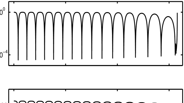
Figure 2: Secular evolution of $\epsilon=1-e^{2}_{1}$ of the inner binary and mutual inclination angle $I$ between the inner and outer binaries. This evolution was computed by integrating equations (16)–(19) which include contributions from Kozai mechanism, PN periastron precession, and gravitational radiation reaction. The initial system parameters are: $m_{0}=m_{1}=m_{2}=10$ $M_{\odot}$, $e_{1}=e_{2}=0.1$, $a_{1}=10$ AU, $a_{2}/a_{1}=10$, $g_{1}=0$, and $I_{0}=95.3^{o}$. This is a typical case in which the PN effect becomes important before the GR effect dominates in the evolution of $\epsilon$, and that the system merges after many Kozai cycles.

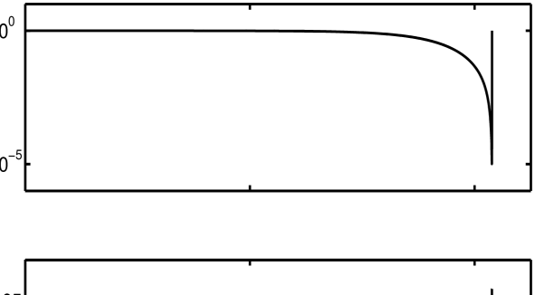
Figure 4: Secular evolution for $\epsilon$ of the inner binary and of $I$, as computed by integrating the evolution equations (16)–(19) which include contributions from the Kozai mechanism, PN periastron precession, and gravitational radiation reaction. The initial system parameters are: $m_{0}=m_{1}=m_{2}=5$ $M_{\odot}$, $e_{1}=0.01,e_{2}=0.51$, $a_{1}=2.1920$ AU, $a_{2}/a_{1}=5$, $g_{1}=0$, and $I_{0}=99.2^{o}$. This is a typical case where the GR effect dominates in the evolution within one Kozai cycle.

The numerical evolutions of $\epsilon$ and $I$ are shown for two typical examples in Fig. 2 and in Fig. 4 for illustration. These evolutions were obtained by integrating the ordinary differentiation equations (16)-(19) for given initial data and then using equation (2) to derive the mutual inclination angle $I$. We used a medium order Runge-Kutta method (available in Matlab as ode45) for the integration.

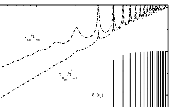
Figure 3: Evolution of $\epsilon$ (solid line) and the time scales of gravitational merger and the PN effect (dashed-dotted lines) with the semimajor axis $a_{1}$ for the same initial parameters and evolution equations as in Fig. 2. The evolution path of $\epsilon$ starts from the upper right of the solid line and moves towards the left. The upper and lower limits on $\epsilon_{\rm min}(a_{1})$ based on equations (11) and (31) (dashed lines) are also shown.

The first example (Fig. 2) represents a case in which the system merges after many Kozai cycles. This is also a case where the PN effect becomes important before the GR effect dominates in the evolution of $\epsilon$. The system parameters are chosen to be $m_{0}=m_{1}=m_{2}=10$$M_{\odot}$, $e_{1}=e_{2}=0.1$, $a_{1}=10$ AU, $a_{2}/a_{1}=10$, $g_{1}=0$, and $I_{0}=95.3^{o}$. The gradual increase in the time scale of the Kozai cycle is apparent. For most of the cycles, $e_{\rm max}\sim 1$ ($\epsilon_{\rm min}$ $\sim 0$). Near the $\epsilon_{\rm min}$  of the last Kozai cycle, fast damped oscillations of $\epsilon$ (and $I$) due to the PN periastron precession are visible before a monotonically increase of $\epsilon$ due to the dominating GR effect (see also Fig. 3). The value of $I$ experiences damped oscillation after the PN effect becomes important and converges to a constant after the GR effect dominates in the evolution. Note also that before the last cycle, the minimum $I$ is around $39^{o}$ as predicted by equation (12).

We show in Fig. 3, for the first example, the evolution of $\epsilon$ with $a_{1}$ (solid line) and compare with the results based on the lower limit of $a_{1}$$\epsilon_{\rm min}$ obtained with equation (38) and a upper limit that is three times this lower limit as discussed in section 3.3 (dashed lines). Also shown in dashed-dot lines are the evolutions of the time scales of the GR and the PN effects normalized by the Kozai time scale $\tau^{{}^{\prime}}_{\rm evol}$. The evolution path of $\epsilon$ starts from the upper right of the solid line and moves towards the left. It is apparent that $a_{1}$ remains essentially a constant within each cycle before $\tau_{\rm GR}/\tau^{{}^{\prime}}_{\rm evol}\sim 1$. The decay of $a_{1}$ occurs mainly near $\epsilon_{\rm min}$ of each cycle. Damped oscillations are apparent near $\tau_{\rm PN}/\tau^{{}^{\prime}}_{\rm evol}\sim 1$. There is an excellent agreement between our numerical results and the prediction in sections 3.2-3.3.

The second example (Fig. 4) represents a case where the system merges within the first Kozai cycle. The system parameters are chosen to be $m_{0}=m_{1}=m_{2}=5$$M_{\odot}$, $e_{1}=0.01$, $e_{2}=0.51$, $a_{1}=2.1920$ AU, $a_{2}/a_{1}=5$, $g_{1}=0$, and $I_{0}=99.2^{o}$. This is a case similar to the classical $\alpha=\beta$ case. That is, the system evolves along $\epsilon\approx 1$ until it passes through an unstable stationary point at $g_{1}\sim\sin^{-1}\sqrt{2/5}\sim 39^{o}$ and then evolves towards extremely small values of $\epsilon$ (Fig. 5, solid line with open circles). The evolution is then quickly dominated by the gravitational radiation reaction near $\epsilon_{\rm min}$.

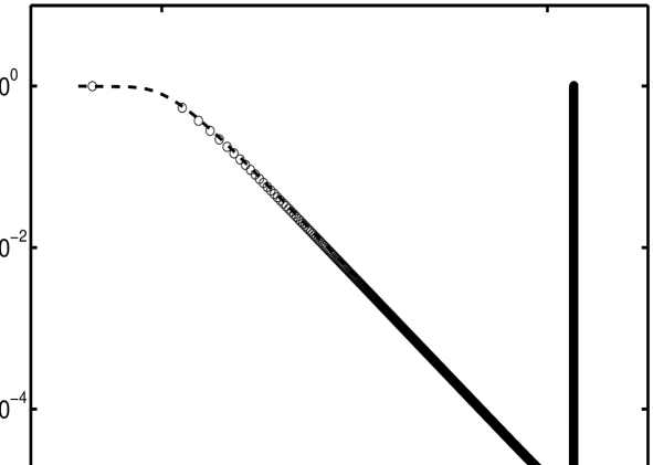
Figure 6: Evolution of $\epsilon$ with the semimajor axis $a_{1}$ (open circles) for the same initial parameters and evolution equations as in Fig. 4. Note that the evolution path starts from the upper right and moves towards the left. The predicted $\epsilon_{\rm min}$ by equation (25) at ${a_{1}}_{0}$ is shown by the symbol ‘X’. The predicted evolution of $\epsilon$ vs $a_{1}$ from equations (38) is shown by the dashed line. There is an excellent agreement between the numerical values and the predictions. This is a typical case where the GR effect dominates within one Kozai cycle and the PN effect is negligible.

The evolution of $\epsilon$ with $a_{1}$ (solid circles) for this second example is shown in Fig. 6. The predicted $\epsilon_{\rm min}$ of the first Kozai cycle calculated with the method in section 3.2 at initial $a_{1}={a_{1}}_{0}$ is shown in symbol ‘x’. The expected evolution of $\epsilon$ with $a_{1}$ by equation (38) starting from this predicted $\epsilon_{\rm min}$ and ${a_{1}}_{0}$ is shown by the dashed line. It is clear that there is an excellent agreement between the predicted evolution of $a_{1}$$\epsilon_{\rm min}$ and the numerical values. The same excellent agreement has been found for all such cases we have investigated.

The phase diagram for the evolution path of $\epsilon$ vs $g_{1}$ for systems with the parameters of our second example but with different initial values $I_{0}$ are shown in Fig. 5. It is apparent that as long as $I_{0}$ is away from the critical values $I_{c}$, the $\epsilon_{\rm min}$ is reached around $g_{1}\sim 90^{o}$. Near the critical value, $g_{m}\sim g_{c}$.

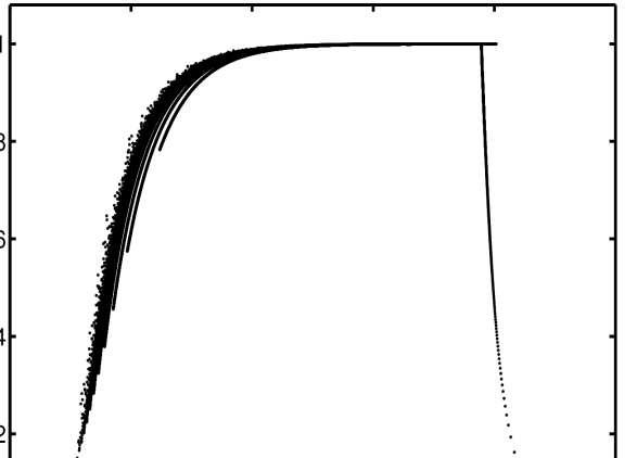
Figure 7: Evolution of $e_{1}$ with gravitational wave frequency $f^{m}_{\rm GW}$ for the system shown in Fig. 2. The $f^{m}_{\rm GW}$ spans eight orders of magnitude. The eccentricity is nearly zero at and above 10 Hz.

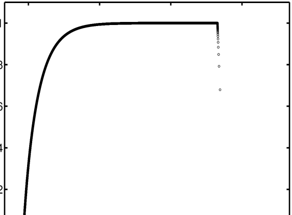
Figure 8: Evolution of $e_{1}$ with $f^{m}_{\rm GW}$ for the system shown in Fig. 4. The $f^{m}_{\rm GW}$ again spans eight orders of magnitude. The eccentricity is around $0.9$ at 10 Hz.

The evolutions of eccentricities $e_{1}$ as a function of gravitational wave frequencies $f^{m}_{\rm GW}$ for our first and second examples are shown in Fig. (7) and (8). In both cases, the GW frequency spans a wide range of eight orders of magnitude. This means that the GW’s from these sources can be good candidates for detections in the LISA band as well as LIGO. For the case of many Kozai cycles in Fig. 7, the eccentricity drops sharply from $e_{1}\sim 1$ at $f_{\rm GW}\sim 0.1$ Hz (the end of the LISA band) where the GR effect starts to dominate, and is nearly zero at 10 Hz (the beginning of the LIGO band). This is expected as equations (37) and (38) predict that the eccentricities drop with the frequency roughly proportional to ${f^{m}}^{-19/18}_{\rm GW}$. For extreme cases as shown in Fig. 8, the eccentricity remains at the significant value of $\sim 0.9$ at $f^{m}_{\rm GW}=10$ Hz and could be extremely high at lower frequencies.

4 Eccentricity Distribution

The Kozai mechanism can drive the inner binaries of triple systems to extremely small $\epsilon$ and merge before disruption by interactions with field stars. The time scale for disruption (the same as the stellar encounter time scale) is given as (Miller & Hamilton (2002))

$$\tau_{\rm enc}\approx 6\times 10^{5}n^{-1}_{6}\frac{\rm AU}{a_{2}}\frac{10\mbox{$M_{\odot}$}}{M_{2}}\ \mbox{yr},$$ (39)

where the number of stars in the globular cluster is $N=10^{6}n_{6}$. We assume $n_{6}=1$ in this paper. Successful mergers of this sort therefore require

$$\tau_{\rm evol}<\tau_{\rm enc},$$ (40)

$$\frac{\tau_{\rm GR}(a_{1},\epsilon_{\rm min})}{\sqrt{\epsilon_{\rm min}}}<\tau_{\rm enc}.$$ (41)

Equation (40) ensures that the system has completed at least a half Kozai cycle to reach small $\epsilon$. Equation (41) ensures that the system can merge successfully before the next interruption. The term on the left-hand side of equation (41) represents the total lifetime of the system which is roughly a factor of $1/\sqrt{\epsilon_{\rm min}}$ the merger time scale $\tau_{\rm GR}$. This is because the system only spends a significant fraction of $\sqrt{\epsilon_{\rm min}}$ its time near $\epsilon_{\rm min}$ where the GR effect is the strongest.

4.1 Distribution of Initial $\epsilon_{\rm min}$  and $a_{1}$

We have explored the parameter space of $\epsilon_{\rm min}$  and $a_{1}$ for successful mergers driven by the Kozai mechanism in globular clusters restricting ourselves to a triple system consisting of three 10 $M_{\odot}$ BHs. We fix the initial parameters $g_{1}=0$, and ${e_{1}}_{0}={e_{2}}_{0}=0.01$, and we have chosen $a_{2}/a_{1}=[20,10,5,3]$ and assume a uniform distribution in the initial mutual inclination angles $I_{0}$ and in the semimajor axis $a_{1}$. The minimum initial value of $a_{1}$ was set to $0.2$ AU so that during its interaction with a third body, the recoil velocity associated with binary hardening is low enough for the system to remain in the cluster (Miller & Hamilton (2002)). There was no presumed upper limit for $a_{1}$. For each given $a_{1}$, $I_{0}$, and $a_{2}/a_{1}$, we first calculated $\epsilon_{\rm min}$  with equation (25) for each given $a_{1}$ and $I_{0}$. Equations (40) and (41) were then evaluated to determine the permitted parameter space.

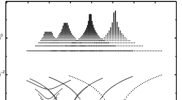
Figure 9: Parameter space for $a_{1}$ (upper set) and corresponding values of $\epsilon_{\rm min}$ (lower set) vs $I_{0}$ for $a_{2}/a_{1}=20,10,5,3$ from left to right (see text).

We show in Fig. 9 the permitted values for $a_{1}$ (upper set) and corresponding $\epsilon_{\rm min}$ (lower set) vs $I_{0}$. There are four sets of cone-shaped distributions, each corresponding to a given $a_{2}/a_{1}$, with value decreasing from the left to the right. Each distribution centers on the critical value $I_{0}\sim I_{c}$ which depends solely on $a_{2}/a_{1}$ (eq. [3]) as $\epsilon_{0}$ is fixed. There is a cut-off at a maximum $a_{1}$. This cut-off in $a_{1}$ is set by the constraint from equation (40). For a fixed $a_{2}/a_{1}$, larger $a_{1}$ implies larger $a_{2}$ and therefore shorter $\tau_{\rm enc}$ (eq. [39]). Beyond the maximum $a_{1}$, the time scale $\tau_{\rm enc}$ becomes so short that the system is disrupted before it can finish a half Kozai cycle to reach $\epsilon_{\rm min}$. For the same reason, a larger $a_{2}/a_{1}$ leads to smaller cut-off in $a_{1}$.

The overall cone shape in $a_{1}$ and $\epsilon_{\rm min}$  results from the fact that the merger time scale should be less than the encounter time scale (eq. [41]). Near the center of the cone where $I_{0}\sim I_{c}$, the system can reach extremely small $\epsilon_{\rm min}$ (eq. [8]) which allows maximum possible values of $a_{1}$ under the constraint of equation (41). The further $I_{0}$ is away from the center ($I_{c}$), the larger $\epsilon_{\rm min}$ is, and so the smaller are the $a_{1}$ values that satisfy equation (41).

The range of $\epsilon_{\rm min}$ within each distribution is caused by the PN effect. In the classical limit (with no GR or PN effect), $\epsilon_{\rm min}$ depends only on the values of $I_{0}$ and $a_{2}/a_{1}$. It is independent of $a_{1}$ for each distribution, making $\epsilon_{\rm min}$  have a unique value at each $I_{0}$. This is apparent for $\epsilon$ at $I_{0}$ far away from center of each distribution for $a_{2}/a_{1}=3,5,10$ in Fig. 9. A significant contribution from the PN effect makes $\epsilon_{\rm min}$ depend on $a_{1}$, giving $\epsilon_{\rm min}$ a finite range (eq. [5],[8]). The PN effect is especially pronounced near the center of each cone ($I_{0}\sim I_{c}$), where the contribution from the classical Hamiltonian is relatively smaller (eq. [8]). The finite range of $\epsilon_{\rm min}$  is more pronounced for cones with larger $a_{2}/a_{1}$ values as the PN effect is more pronounced at larger $a_{2}/a_{1}$. This also explains the overall large $\epsilon_{\rm min}$ at larger $a_{2}/a_{1}$.

The $\epsilon_{\rm min}$ values estimated including the GR effect can be several orders of magnitude larger than those without the GR effect in the region $I_{0}\sim I_{c}$, where the GR effect is the strongest. This makes little difference in finding the permitted parameter space for $a_{1}$, as $\epsilon_{\rm min}$ will be extremely small in this region and equations (41) will be satisfied in either case. However, the evolution of gravitational wave frequency depends sensitively on our knowledge of $a_{1}$$\epsilon_{\rm min}$. It is therefore necessary to include the GR effect.

4.2 Distribution of Eccentricities in the LIGO band

We proceed to investigate the distribution of eccentricities when the emitted GW wave enters the LIGO band. We restrict attention to stellar mass black holes in triple systems and show only a representative case of triple systems consisting of three 10 $M_{\odot}$ black holes. We consider a uniform distribution of initial mutual inclination angle $I_{0}$, initial eccentricities of the inner and outer binaries, ratios of the semimajor axis $a_{2}/a_{1}$, and initial $g_{1}$. A summary of the parameter space we have investigated and the representative values we have included can be found in Table 1.

We choose the upper limit of $a_{2}/a_{1}$ to be 30 based on equations (40), as the parameter range for $a_{1}$ diminishes with larger $a_{2}/a_{1}$ (see Fig. 9). A general upper limit for the ratio $a_{2}/a_{1}$ can also be set based on the requirement that $\epsilon_{0}\geq\epsilon_{\rm min}$; it follows from equation (8) that

$$\frac{a_{2}}{a_{1}}<399\left(\frac{a_{1}}{\rm AU}\right)^{1/3}\frac{\left(m_{2}/\mbox{$M_{\odot}$}\right)^{1/3}}{(M_{1}/\mbox{$M_{\odot}$})^{2/3}}\frac{\epsilon^{1/6}_{1}}{\epsilon^{1/2}_{2}}.$$ (42)

This expression is similar to the limit given by Blaes, Lee & Socrates (2002) (eq. [5]) with a slight difference in the constant term and difference in the power of $\epsilon$ ( $1/6$ here vs $1/2$ there). The lower limit for $a_{2}/a_{1}$ is set to be 3 based on the fact that the triple system is stable only if (Mardling & Aarseth (2001)),

$$\frac{a_{2}}{a_{1}}>2.8\left[\left(1+\frac{m_{2}}{M_{1}}\right)\frac{1+e_{2}}{(1-e^{2}_{2})^{1/2}}\right]^{2/5}.$$ (43)

We follow the same procedure described in the previous subsection. We first calculate the permitted parameter space for $\epsilon_{\rm min}$ and $a_{1}$. The results (not shown) are many versions of the same distributions of those shown in Fig. 9 for various $a_{2}/a_{1}$. The span of permissible $I_{0}$ is roughly 90–106^o, as required to obtain extremely small $\epsilon_{\rm min}$. We then calculate the expected eccentricity $e_{1}$ or its upper and lower limit at given frequency following the numerical procedures described in section 3.4, taking into account of both the GR and PN effects.

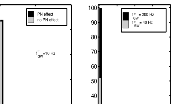
Figure 10: The distribution of eccentricities at $f^{m}_{\rm GW}=10$ Hz (left panel) and 40 Hz, 200 Hz (right panel) for black hole mergers driven by the Kozai effect in a globular cluster. See Table 1 for the parameter ranges used. Each parameter is uniformly distributed in its range unless specified.

The number distribution of eccentricities at $f^{m}_{\rm GW}\sim 10$ Hz is shown as a histogram in the left panel of Fig. 10. The distribution is shown in percentage relative to the total number of systems that would merge before interruption by field stars. The histogram in grey shade represents the distribution without considering the impact of the PN effect on the evolution of $a_{1}$$\epsilon_{\rm min}$ (see discussions in section 3.3). The histogram in dark shade includes the upper limit due to the impact of the PN effect. The x-axes of the histograms is shifted for a better view. It is apparent that the PN effect affects mostly the low-eccentricity systems and it makes little difference in the histogram.

At $f^{m}_{\rm GW}=10$ Hz, around $70\%$ of the merger systems have eccentricity $<0.1$, a little more than 50% have eccentricities $<0.05$. About $\sim 2$ % have eccentricities $e_{1}\sim 1$, most of which are those with initial $I_{0}$ very close to the critical angle $I_{c}$, as the GW’s reach 10 Hz before the systems reach $\epsilon_{\rm min}$ within the first Kozai cycle. These are the type of systems studied in Fig. 4, 5, 6, and 8.

We also show eccentricity distributions in the right panel of Fig. 10 for $f^{m}_{\rm GW}=40$ Hz (grey shade) and $f^{m}_{\rm GW}=200$ Hz (dark shade). At 40 Hz, all eccentricities are well below 0.2. At 200 Hz, all are well below 0.02. This is not surprising as equations (37) and (38) predict that the eccentricities drop with the frequency roughly proportional to ${f^{m}}^{-19/18}_{\rm GW}$. This is consistent with the fact that the GR effect circularizes the system in a very rapid fashion.

5 Discussion

We have studied the evolution of eccentricities of black hole mergers driven by the Kozai mechanism in triple systems residing within globular clusters. Eccentricity distributions at gravitational wave frequencies relevant to LIGO have been presented. The evolution of these systems were investigated including the Kozai mechanism, the post-Newtonian periastron precession effect, and gravitational radiation reaction.

We conclude that around 30% of the systems possess eccentricities $>0.1$ when the emitted gravitational waves reach 10 Hz. Around 2% of the systems are extremely eccentric at 10 Hz. However almost all our merger systems possess eccentricities well below 0.2 at 40 Hz, and below 0.02 at 200 Hz (see also a brief discussion in Miller 2002). These merger systems, on the other hand, promise extremely high eccentricities at the lower frequencies of the LISA band (see Fig. [7],[8]).

About 30% of our merger systems possess $e>0.1$ at 10 Hz, the lower end of the advanced LIGO frequency band (Fritschel (2002)). It is thus important to determine whether it is possible to use LIGO’s current circular-binary search templates to detect such systems. For highly eccentric systems, the higher harmonics probably need to be taken into account when optimizing the search templates. It is plausible that the eccentricities associated with these systems are not important at 200 Hz or perhaps even at 40 Hz. It is important however, to determine the limit of $e_{1}$ below which, circular-binary templates need to be replaced by new, eccentric-binary templates (see Martel & Poisson (1999)).

The eccentricity distribution was calculated for triple systems consisting of three 10 $M_{\odot}$ black holes. Similar eccentricity distribution, however, can be found for triple systems with individual masses in the range of 3–25 $M_{\odot}$ known for the observed galactic stellar mass BHs (Bailyn, Jain, Coppi, & Orosz (1998)). We have assumed that, in globular clusters, triple systems with one or more BHs of mass $>25$$M_{\odot}$ are rare. The mass parameters affect very little the values of $\epsilon_{\rm min}$ a system can reach (eq. [8],[5],[24]). Its effect to the shape of eccentricity distribution is also very weak compared with other parameters such as $a_{1}$, $a_{2}/a_{1}$, and $\epsilon$ (eq. [40], [41]). Any effects due to different masses will be further averaged out if we include a uniform distribution of masses within this range.

Our calculation of the gravitational radiation reaction is based on the Newtonian quadrupole approximation. At 10 Hz, this approximation is still valid as $v/c\sim 0.1$ at the periastron. However, at higher frequencies, especially near 200 Hz in the LIGO frequency band, this approximation breaks down as the speed of the binary orbit is approaching that of light. However, all our binaries become so circular well before they reach 200 Hz, that our results are probably still relevant.

                                                                                                                                             

Figure 1: Geometry of a hierarchical triple system.

                                                                                                                                             

                                                                                                                                             

                                                                                                                                             

                                                                                                                                             

                                                                                                                                             

                                                                                                                                             

                                                                                                                                             

                                                                                                                                             

                                                                                                                                             

Table 1: Parameter ranges investigated for Kozai-mechanism-driven BH mergers in globular cluster

$M_{\rm BH}$ ($M_{\odot}$)	$a_{1}$ (AU)	$a_{2}/a_{1}$	$e_{0}$	$g_{1}(^{o})$	$I_{0}(^{o})$	$n_{6}$
10	0.2–30	3,5,10,20,30	0.01–0.901	0–90	85–110	1

Note. — $M_{\rm BH}$ refers to black hole masses for all three components; $e_{0}$ refers to eccentricities for both inner and outer binaries. Numbers of steps for $a_{1}$, $e_{0}$, $g_{1}$, and $I_{0}$ are 60, 4, 4, and 100 respectively. See the text for definitions.

References

- Bailyn, Jain, Coppi, & Orosz (1998) Bailyn, C. D., Jain, R. K., Coppi, P., & Orosz, J. A. 1998, ApJ, 499, 367
- Blaes, Lee, & Socrates (2002) Blaes, O., Lee, M. H. & Socrates, A. 2002, ApJ, accepted, astro-ph/0203370
- Buonanno, Chen, & Vallisneri (2002) Buonanno, A. Chen, Y. & Vallisneri, M. 2002, gr-qc/0205122
- (4) Ford, E. B., Kozinsky, B., & Rasio, F. A. 2000, ApJ, 535, 385
- Fritschel (2002) Fritschel, P. 2002, to appear in Proceedings of SPIE, 4856, Gravitational Wave Detection, Waikoloa, HI, 2002, available at http://www.ligo.caltech.edu/docs/P/P020016-00.pdf
- Glampedakis, Hughes, & Kennefick (2002) Glampedakis, K., Hughes, S. & Kennefick, D. 2002 Phys. Rev. D, submitted, gr-qc/0205033
- Gopakumar & Iyer (2002) Gopakumar, A. & Iyer 2002, Phys. Rev. D, 65, 084011
- Kozai (1962) Kozai, Y. 1962, AJ, 67, 9
- Innanen, Zheng, Mikkola, & Valtonen (1997) Innanen, K. A., Zheng, J. Q., Mikkola, S., & Valtonen, M. J. 1997, AJ, 113, 1915
- Lidov & Ziglin (1976) Lidov, M. L. Ziglin, S. L. 1976, Celestial Mechanics, 13, 471
- Lincoln & Will (1990) Lincoln, C. W. & Will, C. M. 1990, Phys. Rev. D, 42, 1123
- Martel & Poisson (1999) Martel, K. & Poisson, E. 1999, Phys. Rev. D, 60, 124008
- Moreno-Garrido, Mediavilla, & Buitrago (1994) Moreno-Garrido, C., Mediavilla, E. & Buitrago, J. 1994, MNRAS, 266, 16
- Moreno-Garrido, Mediavilla, & Buitrago (1995) Moreno-Garrido, C., Mediavilla, E. & Buitrago, J. 1995, MNRAS, 274, 115
- Mardling & Aarseth (2001) Mardling, R. A. & Aarseth, S. J. 2001, MNRAS, 321, 398
- Miller & Hamilton (2002) Miller, C. & Hamilton, D. P. 2002, ApJ submitted, astro-ph/0202298
- Miller (2002) Miller, C. 2002, ApJ submitted, astro-ph/0206404
- Nelder & Mead (1965) Nelder, J. A. & Mead, R. 1965, Computer Journal, 7, 308
- Peters & Mathews (1963) Peters, P. C. & Mathews, J. 1963, Physical Review, 131, 435
- Peters (1964) Peters, P. C. 1964, Physical Review, 136, B1224
- Portegies Zwart & McMillan (2000) Portegies Zwart, S. F. & McMillan, S. L. W. 2000, ApJ, 528, L17
- Scalo (1986) Scalo, J. M. 1986, Fundamentals of Cosmic Physics, 11, 1
- Thorne (1987) Thorne, K. 1987, in “300 years of Gravitation”, eds Hawking, S. W. & Israel, W., Cambridge and New York, Cambridge University Press, 697