Quiet Sun magnetic fields at high spatial resolution

Abstract

We present spectro-polarimetric observations of Inter-Network magnetic fields at the solar disk center. A Fabry-Perot spectrometer was used to scan the two Fe i lines at $\lambda$6301.5 Å and $\lambda$6302.5 Å. High spatial resolution (0$\farcs$5) magnetograms were obtained after speckle reconstruction. The patches with magnetic fields above noise cover approximately 45 % of the observed area. Such large coverage renders a mean unsigned magnetic flux density of some 20 G (or 20 Mx cm^-2), which exceeds all previous measurements. Magnetic signals occur predominantly in intergranular spaces. The systematic difference between the flux densities measured in the two iron lines leads to the conclusion that, typically, we detect structures with intrinsic field strengths larger than 1 kG occupying only 2% of the surface.

1 Introduction

We study magnetic fields of the quiet Sun. Our analysis will exclude the magnetism in photospheric network regions known to contain strong kG magnetic fields (e.g., Stenflo 1994). We will concentrate on the low flux features in the interior of the network which we will call, for brevity, IN fields (Inter-Network fields). Magnetic fields within the network cells were already discovered in the seventies (Livingston & Harvey 1975; Smithson 1975). During the last decade, with improved observational and diagnostic capabilities, these IN fields have obtained increasing attention. They will allow to test our ideas on the magnetic field generation by convective processes, a natural step towards understanding the principles of astrophysical dynamos (e.g. Cattaneo 1999; Emonet & Cattaneo 2001). In addition, it has been found that the very quiet IN areas harbor a sizeable fraction of the solar magnetic flux (see, e.g., Stenflo 1982; Yi et al. 1993; Socas-Navarro & Sánchez Almeida 2002). Such estimates are based on lower limits to the still unknown amount of flux, which suggests the potential importance of the IN component of the solar magnetism.

So far only a fraction of the IN field has been detected. This conclusion follows from the presence of unresolved mixed polarities in 1″ angular resolution observations (e.g., Sánchez Almeida et al. 1996; Sánchez Almeida & Lites 2000; Lites 2002). The mixing of polarities reduces the polarization, making the magnetic structures difficult to identify. Consequently, it is to be expected finding more sites with magnetic fields when increasing the spatial resolution. This idea triggered our investigation: we aimed at observing the IN fields with the highest possible spatial resolution yet keeping a good polarimetric sensitivity.

Many of the recent observational studies find that the IN fields have magnetic field strengths substantially lower than 1 kG (Keller et al. 1994; Lin 1995; Lin & Rimmele 1999; Bianda et al. 1998; Bianda et al. 1999; Khomenko et al. 2002). Yet, on the basis of different observing and interpretation techniques, one can find in IN areas strong kG magnetic fields (Grossmann-Doerth et al. 1996; Sigwarth et al. 1999; Sánchez Almeida & Lites 2000; Socas-Navarro & Sánchez Almeida 2002). This seeming discrepancy probably points out that the IN regions present a continuous distribution of field strengths. Depending on the specificities of the diagnostic technique, one selects only a particular part of such distribution (see Cattaneo 1999; Sánchez Almeida & Lites 2000).

In this study we confirm the presence of kG IN magnetic fields. In addition, we detect an amount of unsigned magnetic flux which exceeded any value previously reported in the literature. Our conclusions are based on spectro-polarimetric observations achieving both high spatial resolution (0$\farcs$5) and fair sensitivity (20 G). In this letter we give a short description of the observations and the data analysis. Our aim is to communicate the results bearing on strong IN fields and large flux densities. A detailed discussion, including additional properties on the time evolution, will be given in a forthcoming more extended contribution.

2 Observations and data reduction

The observations were obtained in April 2002 with the Göttingen Fabry-Perot Interferometer (FPI; Bendlin et al. 1992; Bendlin 1993) mounted at the Vacuum Tower Telescope of the Observatorio del Teide (Tenerife). The seeing was excellent (Fried parameter $r_{0}$ = 13–14 cm). A very quiet region near disk center was selected using G band video images to avoid network regions. The observational setup is described in Koschinsky et al. (2001), which includes a Stokes $V$ polarimeter. While scanning across a spectral region, the spectrometer takes two-dimensional narrow-band images with short exposure times and, strictly simultaneously, broadband images from the same Field Of View (FOV).

The data for the present study stem from a 17 mininutes time series of spectral scans in the 6302 Å region, containing the Fe i $\lambda$6301.5 Å line (Landé factor $g=1.67$), the Fe i $\lambda$6302.5 Å line ($g=2.5$), and the telluric O₂ 6302.76 Å line. The FWHM of the FPI and the sampling interval were 44 mÅ and 32 mÅ, respectively. Each FPI scan consists of 28 wavelength positions for the two iron lines, and 5 wavelength positions for the telluric line. The duration of a spectral scan is 35 s, plus 15s needed for storage onto hard disk. The FOV corresponds to 15″$\times$25″on the Sun, sampled with a pixel size of 0$\farcs$1$\times$0$\farcs$1. The data reduction includes subtraction of dark current, flat fielding, and speckle reconstruction of the broadband images (de Boer & Kneer 1992; de Boer 1996) using the spectral ratio method (von der Lühe 1984) and the speckle masking method (Weigelt 1977). The reconstruction of the narrow-band images proceeds the way proposed by Keller & von der Lühe (1992; see also Krieg et al. 1999; Hirzberger et al. 2001). We use the code by Janßen (2003) with minor modifications. To have the noise filtering independent of the seeing, which may vary during a spectral scan, we apply a filter which limits the spatial resolution of the reconstructed spectro-polarimetric images to 0$\farcs$5. To further suppress noise, the images were processed with a 5$\times$5 pixel boxcar smoothing after the filtering. The FPI simultaneously collects the left and right circularly polarized beams onto different areas of the CCD. They are added and subtracted to obtain the Stokes $I$ and $V$ profiles. This task demands a careful superposition of the two beams, which we carry out after a sub-pixel interpolation. The spatial filters were not applied to the broad-band images.

2.1 Calibration of the magnetograms

Magnetic flux densities are computed starting from the magnetograph equation, which relates the circular polarization $V$ and the longitudinal component of the magnetic field $B$ (e.g., Unno 1956; Landi Degl’Innocenti 1992),

$$V(\lambda)=C(\lambda)\ B,$$ (1)

with the calibration constant $C(\lambda)$ proportional to $dI(\lambda)/d\lambda$. First, the derivative of Stokes $I$ required to evaluate $C(\lambda)$ is computed numerically for each iron line. Then, the wavelengths of the two extrema of the derivative, plus the two wavelengths immediately adjacent to each one of them, are selected. The flux density of each solar point, $B_{\mathrm{eff}}$, is obtained solving equation (1) for these six wavelengths $\lambda_{i}$. The least-squares fit renders

$$B_{\mathrm{eff}}=\sum_{i}V(\lambda_{i})\ C(\lambda_{i})\Big{/}\sum_{i}C^{2}(\lambda_{i}).$$ (2)

Obviously, if the observed Stokes $I$ and $V$ profiles satisfy equation (1) then $B_{\mathrm{eff}}=B$. In general this is not the case and $B_{\mathrm{eff}}$ represents a mere biased estimate of the true flux density.

Two main sources of noise limit the precision of $B_{\mathrm{eff}}$. The measure is affected by the random noise of the Stokes $V$ spectra. We estimate its influence applying to equation (2) the law of propagation of errors (e.g., Martin 1971). Assuming the Stokes $V$ noise to be constant and equal to $0.5\%I_{c}$ ($I_{c}$ being the continuum intensity), the typical value for the random error of $B_{\mathrm{eff}}$ turns out to be 20 G (Table 1; 1 G $\equiv$ 1 Mx cm^-2). The adopted $V$-noise comes from the r.m.s. fluctuations of the Stokes $V$ profiles when $B_{\mathrm{eff}}\longrightarrow 0$. A second source of error affecting $B_{\mathrm{eff}}$ is due to the contamination of the polarization signals with intensity (the so-called $I$-to-$V$ crosstalk). It can be created in many ways during the reduction procedure (e.g., errors in setting the continuum intensity level). Since $V\ll I$, a small crosstalk compromises the polarimetric accuracy of the measurements. Fortunately, the procedure that we employ to determine $B_{\mathrm{eff}}$ is insensitive to this contamination. The calibration constant $C(\lambda)$ has different signs in the two wings of the spectral lines, consequently, any symmetric contribution to $V$ (e.g., the contamination with Stokes $I$) leaves only a small residual in equation (2). Using quiet Sun Stokes $I$ profiles, we deduce a residual of at most a few G, which is regarded as negligible.

3 Results and discussion

3.1 Magnetograms

Figure 1 presents two magnetograms taken simultaneously in the two iron lines. They exhibit a salt and pepper pattern. The close similarity of the two magnetograms demonstrates that we have found magnetic field signals above noise. We sought and found further evidences for the consistency of the magnetograms. Among them (a) most of the patches have sizes of the resolution limit or larger, and (b) the patches maintain their identity between successive snapshots of the time sequence that we obtained. Approximately 45 % of the FOV contains polarimetric signal. The mean unsigned magnetic field density averaged over the FOV is 21 G, for the magnetogram based on Fe i $\lambda$6301.5 Å, and 17 G for Fe i $\lambda$6302.5 Å (Table 1). In this average we set to zero all those pixels with $B_{\mathrm{eff}}$ below the noise level. The unsigned flux densities that we measure are larger than the values found hitherto (e.g., see the values compiled by Sánchez Almeida et al. 2003, §4.1). We detect more signals probably due to the unique combination of high spatial resolution and good sensitivity of our observation. The magnetic flux detected in the IN critically depends on the polarimetric sensitivity and the angular resolution. For example, if the magnetograms in Figure 1 had a sensitivity of 100 G, then the mean unsigned flux density drops to 1-2 G (Table 1; the new lower sensitivity is modeled setting to zero all the observed signals below 100 G). The drastic decrease of signals with decreasing sensitivity can easily explain why the IN signals that we detect have been missed in previous high resolution magnetograms (Keller 1995; Stolpe & Kneer 2000; Berger & Title 2001). A decrease of angular resolution also reduces the signals due to cancellation between close opposite polarities. If the angular resolution of the observation is artificially degraded by convolving the magnetograms in Figure 1 with a 1″ FWHM Gaussian, then the mean unsigned flux densities become of the order of 7-9 G. These values agree with previous determinations based on scanning spectro-polarimeters that reach 1″ resolution (Sánchez Almeida & Lites 2000 obtain 10 G, whereas Lites 2002 gives 9 G). The mean signed magnetic flux density in Figure 1 is found to be +3 G for Fe i $\lambda$6302.5 Å, and +2 G for Fe i $\lambda$6301.5 Å.

Figure 2 shows the speckle reconstructed broad-band image and, overlaid to it, the Fe i $\lambda$6302.5 Å magnetogram. It is important to note that most of the magnetic fields, $\approx 65$ %, are located in intergranular spaces. This was observed before (Lin & Rimmele 1999; Lites 2002; Socas-Navarro 2003) and is expected from numerical simulations of magneto-convection (e.g., Cattaneo 1999). Our high spatial resolution observations leave no doubt on these results. However, magnetic fields can also be found in granules (Stolpe & Kneer 2000; Koschinsky et al. 2001). Patches of opposite polarity are often located close to each other, again in agreement with expectations from numerical simulations.

3.2 Magnetic field strengths

The polarization signals obtained from the two spectral lines are correlated (see Fig. 1). However, the magnitude of the effective flux density of Fe i $\lambda$6301.5 Å, $B_{\mathrm{eff}}(6301)$, is systematically larger than the effective field derived using Fe i $\lambda$6302.5 Å, $B_{\mathrm{eff}}(6302)$. We have estimated this excess by several means: least-squares fit of $B_{\mathrm{eff}}(6301)$ versus $B_{\mathrm{eff}}(6302)$, least-squares fit of $B_{\mathrm{eff}}(6302)$ versus $B_{\mathrm{eff}}(6301)$, mean ratio among all points in the field of view, etc. Our best estimate for this ratio is,

$$B_{\mathrm{eff}}(6301)/B_{\mathrm{eff}}(6302)\simeq 1.28\pm 0.10,$$ (3)

where the error bar accounts for all the individual estimates. We interpret this systematic difference as an indication that the magnetic field strengths in the magnetograms are, typically, in the kG regime. For weak fields, say 500 G, the magnetograph equation (1) holds, since the basic conditions for the approximation to be valid are satisfied (Socas-Navarro & Sánchez Almeida 2002). Thus, for weak fields one expects $B_{\mathrm{eff}}(6301)/B_{\mathrm{eff}}(6302)\simeq 1$. Since this is not the observed ratio, one is forced to conclude that the field strengths have to be in the kG range. We have modeled the ratio (3) using synthetic polarized spectra formed in atmospheres whose magnetic fields are known. Such numerical calibration confirms the qualitative argument posed above, namely, that the ratio (3) corresponds to kG fields.

Note that structures with intrinsic kG magnetic field strength showing 20 G flux density have to occupy only a small fraction of the solar surface. The simplest estimate yields 2% of the area, which comes from fill factor $\sim B_{\mathrm{eff}}/B\sim 20~{}{\rm G}/1000~{}$G.

Magnetic structures with kG fields should be bright at the granulation level because they have lower density and thus lower opacity than the ambient atmosphere (Spruit 1976). Except for a few cases (e.g., Fig. 2, upper left corner at [1$\farcs$5, 22″]), we do not see such brightening in the broadband images. This implies that the structures must thus be smaller than the resolution of these images, of approximately 0$\farcs$25 or 180 km.

4 Conclusion

We have demonstrated that polarimetric observations with high spatial resolution reveal a wealth of magnetic structures even in the very quiet Sun, away from activity or network features. Our study reveals a mean unsigned flux density of 20 G, which is at least a factor two larger than the flux found in previous studies having lower angular resolution. Even more, it is almost twice the flux density detected during the solar maximum in the form of active regions and network using conventional techniques (see Socas-Navarro & Sánchez Almeida 2002; Sánchez Almeida 2002). Our analysis also leads to the conclusion that the IN fields contain strong kG fields. Since only some 2% of the solar surface produces these kG signals, we do not exclude the existence of weaker fields in the region (of the order of tens of G, as found from Hanle diagnostics, or hundreds of G, as deduced from Fe i 15648 Å measurements; see §1).

We find no evidence that the angular resolution and sensitivity of our magnetograms suffice to single out all the magnetic features existing in the IN region. Consequently, the flux that we detect should be regarded only as a lower limit.

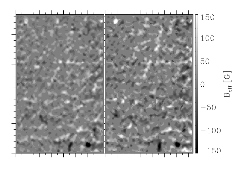
Figure 1: Magnetograms in the two Fe i lines at $\lambda$6302.5 Å (left) and $\lambda$6301.5 Å (right). Dark and light correspond to different polarities (see the vertical bar). The distance between tickmarks is 1″.

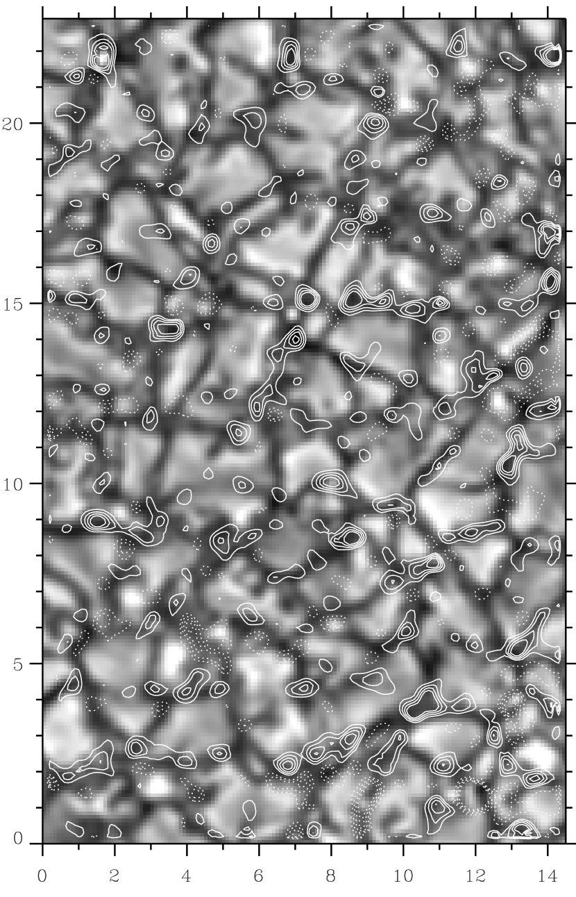
Figure 2: Speckle reconstructed broadband image overlaid with the magnetogram of Fe i $\lambda$6302.5 Å with contours at $|B_{\mathrm{eff}}|=$ 30, 50, 70, and 90 G. The solid and dotted contours indicate opposite polarities. The distance between tickmarks is 1″.

Table 1: Mean unsigned flux density in the magnetograms

line	full data	$>100$ G	1″ seeing	signed flux	random noise
Fe i $\lambda$6301.5 Å	21 G	2 G	9 G	2 G	23 G
Fe i $\lambda$6302.5 Å	17 G	1 G	7 G	3 G	17 G

References

- Bendlin (1993) Bendlin, C. 1993, Ph.D. thesis, University of Göttingen, Göttingen
- Bendlin et al. (1992) Bendlin, C., Volkmer, R., & Kneer, F. 1992, A&A, 257, 817
- Berger & Title (2001) Berger, T. E., & Title, A. M. 2001, ApJ, 553, 449
- Bianda et al. (1998) Bianda, M., Stenflo, J. O., & Solanki, S. K. 1998, A&A, 337, 565
- Bianda et al. (1999) Bianda, M., Stenflo, J. O., & Solanki, S. K. 1999, A&A, 350, 1060
- Cattaneo (1999) Cattaneo, F. 1999, ApJ, 515, L39
- de Boer (1996) de Boer, C. R. 1996, A&AS, 120, 195
- de Boer & Kneer (1992) de Boer, C. R., & Kneer, F. 1992, A&A, 264, L24
- Emonet & Cattaneo (2001) Emonet, T., & Cattaneo, F. 2001, ApJ, 560, L197
- Grossmann-Doerth et al. (1996) Grossmann-Doerth, U., Keller, C. U., & Schüssler, M. 1996, A&A, 315, 610
- Hirzberger et al. (2001) Hirzberger, J., Koschinsky, M., Kneer, F., & Ritter, C. 2001, A&A, 367, 1011
- Janßen (2003) Janßen, K. 2003, Ph.D. thesis, University of Göttingen, Göttingen, in press
- Keller (1995) Keller, C. U. 1995, Rev. Mod. Astron., 8, 27
- Keller et al. (1994) Keller, C. U., Deubner, F.-L., Egger, U., Fleck, B., & Povel, H. P. 1994, A&A, 286, 626
- Keller & von der Lühe (1992) Keller, C. U., & von der Lühe, O. 1992, A&A, 261, 321
- Khomenko et al. (2002) Khomenko, E. V., Collados, M., Solanki, S. K., Lagg, A., & Trujillo-Bueno, J. 2002, A&A, in preparation
- Koschinsky et al. (2001) Koschinsky, M., Kneer, F., & Hirzberger, J. 2001, A&A, 365, 588
- Krieg et al. (1999) Krieg, J., Wunnenberg, M., Kneer, F., Koschinsky, M., & Ritter, C. 1999, A&A, 343, 983
- Landi Degl’Innocenti (1992) Landi Degl’Innocenti, E. 1992, in Solar Observations: Techniques and Interpretation, ed. F. Sánchez, M. Collados, & M. Vázquez (Cambridge: Cambridge University Press), 71
- Lin (1995) Lin, H. 1995, ApJ, 446, 421
- Lin & Rimmele (1999) Lin, H., & Rimmele, T. 1999, ApJ, 514, 448
- Lites (2002) Lites, B. W. 2002, ApJ, 573, 431
- Livingston & Harvey (1975) Livingston, W. C., & Harvey, J. W. 1975, BAAS, 7, 346
- Martin (1971) Martin, B. R. 1971, Statistics for Physicists (London: Academic Press)
- Sánchez Almeida (2002) Sánchez Almeida, J. 2002, in Solar Wind 10, ed. M. Velli, AIP Conf. Proc. (New York: American Institute of Physics), in press
- Sánchez Almeida et al. (2003) Sánchez Almeida, J., Emonet, T., & Cattaneo, F. 2003, ApJ, 585, in press
- Sánchez Almeida et al. (1996) Sánchez Almeida, J., Landi Degl’Innocenti, E., Martínez Pillet, V., & Lites, B. W. 1996, ApJ, 466, 537
- Sánchez Almeida & Lites (2000) Sánchez Almeida, J., & Lites, B. W. 2000, ApJ, 532, 1215
- Sigwarth et al. (1999) Sigwarth, M., Balasubramaniam, K. S., Knölker, M., & Schmidt, W. 1999, A&A, 349, 941
- Smithson (1975) Smithson, R. C. 1975, BAAS, 7, 346
- Socas-Navarro (2003) Socas-Navarro, H. 2003, in Solar Polarization Workshop 3, ed. J. Trujillo-Bueno & J. Sánchez Almeida, ASP Conf. Ser. (San Francisco: ASP), in preparation, revise
- Socas-Navarro & Sánchez Almeida (2002) Socas-Navarro, H., & Sánchez Almeida, J. 2002, ApJ, 565, 1323
- Spruit (1976) Spruit, H. C. 1976, Sol. Phys., 50, 269
- Stenflo (1982) Stenflo, J. O. 1982, Sol. Phys., 80, 209
- Stenflo (1994) Stenflo, J. O. 1994, Solar Magnetic Fields, ASSL 189 (Dordrecht: Kluwer)
- Stolpe & Kneer (2000) Stolpe, F., & Kneer, F. 2000, A&A, 353, 1094
- Unno (1956) Unno, W. 1956, PASJ, 8, 108
- von der Lühe (1984) von der Lühe, O. 1984, JOSA, A1, 510
- Weigelt (1977) Weigelt, G. P. 1977, Optics Comm., 21, 55
- Yi et al. (1993) Yi, Z., Jensen, E., & Engvold, O. 1993, in ASP Conf. Ser., Vol. 46, The Magnetic and Velocity Fields of Solar Active Regions, ed. H. Zirin, G. Ai, & H. Wang, San Francisco, 232