Rapid Variability and Annual Cycles in the Characteristic Time-scale of the Scintillating Source PKS 1257326
Abstract
Rapid radio intra-day variability (IDV) has been discovered in the southern quasar PKS 1257326. Flux density changes of up to 40% in as little as 45 minutes have been observed in this source, making it, along with PKS 0405385 and J18193845, one of the three most rapid IDV sources known. We have monitored the IDV in this source with the Australia Telescope Compact Array (ATCA) at 4.8 and 8.6 GHz over the course of the last year, and find a clear annual cycle in the characteristic time-scale of variability. This annual cycle demonstrates unequivocally that interstellar scintillation is the cause of the rapid IDV at radio wavelengths observed in this source. We use the observed annual cycle to constrain the velocity of the scattering material, and the angular size of the scintillating component of PKS 1257326. We observe a time delay, which also shows an annual cycle, between the similar variability patterns at the two frequencies. We suggest that this is caused by a small (as) offset between the centroids of the 4.8 and 8.6 GHz components, and may be due to opacity effects in the source. The statistical properties of the observed scintillation thus enable us to resolve source structure on a scale of microarcseconds, resolution orders of magnitude higher than current VLBI techniques allow. General implications of IDV for the physical properties of sources and the turbulent ISM are discussed.
1 Introduction
Some flat spectrum extragalactic radio sources display variability on time-scales shorter than a day. This phenomenon is known as intraday variability (IDV), and has been studied in detail at cm-wavelengths for two decades (Heeschen 1984; Witzel et al. 1986; see review by Wagner & Witzel 1995). There is now a great deal of evidence that interstellar scintillation (ISS) is the principal mechanism causing IDV to be observed at cm wavelengths (Jauncey et al. 2000; Dennett-Thorpe & de Bruyn 2001, 2002; Rickett et al. 2001, 2002; Jauncey & Macquart 2001). In turn, ISS can be used to probe microarcsecond (as) source structure and properties of the Galactic interstellar medium (ISM) (Macquart & Jauncey, 2002; Rickett, Kedziora-Chudczer & Jauncey, 2002).
PKS 1257326 is a flat-spectrum, radio and X-ray quasar at redshift (Perlman et al., 1998). Its Galactic coordinates are and ecliptic coordinates . Radio IDV was discovered at 4.8 and 8.6 GHz in 2000 June with the Australia Telescope Compact Array (ATCA) during blazar monitoring observations. These observations revealed a compact source showing strong flux density changes over the course of 12 hours. IDV was confirmed in 2000 September. Here we present the results of observations of PKS 1257326 carried out during a year-long monitoring program of a number of the known southern IDV sources (Kedziora-Chudczer et al., 2001A; Bignall et al., 2002) which commenced in 2001 February. Results for the other IDV sources will be presented later. The observations and results are described in Section 2. In Section 3 the analysis of scintillation parameters and source characteristics is presented. Discussion of the evidence for scintillation being the principal mechanism for radio IDV in general, and of the connection between scintillation and intrinsic variability, is presented in Section 4. In Section 5 we discuss the implications of the three known rapid (intra-hour) scintillators for our understanding of cm-wavelength IDV in extragalactic sources. We assume and km s-1 Mpc-1 throughout.
2 The Observations and Results
The ATCA flux density monitoring was carried out simultaneously at 4.80 and 8.64 GHz during 2001 and early 2002, with observing sessions of 48 hours, approximately every six weeks. The target IDV sources were interspersed with a series of compact flux density calibrators, with observations of each source approximately every hour or less, while they were above in elevation. This technique results in well calibrated, accurate and reliable flux density measurements. For PKS 1257326, the time interval between individual measurements was decreased to gain good coverage of its rapid variability. Additional shorter sessions concentrating on this source alone were requested and scheduled.
PKS 1257326 has exhibited IDV from the time it was discovered in 2000 June. Before this time, the only other ATCA data taken on this source were in 1995 October. We have inspected these data, and although they consist of only two brief (1 minute) observations, separated by hours, the two flux density measurements differ by ; it seems the source was also showing rapid IDV at this time. It therefore seems likely that PKS 1257326 has been showing rapid IDV for at least seven years. Figure 1 shows both the 4.8 and 8.6 GHz ATCA flux density measurements from 2001 March 23. The flux density changes remarkably rapidly, from a maximum to a minimum in less than an hour, making PKS 1257326 the third such rapid IDV source known along with PKS 0405385 (Kedziora-Chudczer et al., 1997) and J18193845 (Dennett-Thorpe & de Bruyn, 2000A).
Figure 1 shows the remarkably smooth, quasi-periodic nature of the variability at both frequencies, which we describe by a single time-scale parameter, defined in Section 2.1 below. Also noticeable is the strong correlation between the variations at 4.8 and 8.6 GHz that is a characteristic of many IDV sources, in particular, the other extreme variables (Kedziora-Chudczer et al., 1997; Dennett-Thorpe & de Bruyn, 2000A).
Figure 1 demonstrates the advantage of using the ATCA for such flux density measurements; at these frequencies confusion is negligible, the source is mostly unresolved, and the array gives effectively continuous, dual-frequency, high precision flux density measurements. The data displayed in Figure 1 (and subsequent figures) are averaged over 1 minute and over all baselines. The thermal noise for 1-minute integrations is mJy, neglible compared with the observed variations. The variation of antenna gains with elevation and time contributes an error which is proportional to the flux density. This is well-determined by the calibrator source observations. For the data published here, typical residual proportional errors (peak-to-peak) are up to 1% at 4.8 GHz, and up to 2% at 8.6 GHz.
There is also an error contribution due to extended source structure. Recently we obtained high-resolution, high-sensitivity VLA images of the source which show it has a weak, arcsecond-scale jet (Bignall et al., in preparation). The effect of this has not yet been subtracted from the visibilities in the data published here, however we have determined its contribution. The extended structure adds to the unresolved component a small amount of flux density, which varies over the course of a day as the coverage of the ATCA varies. The contribution is different on different baselines, but the effect tends to be heavily smoothed out by averaging over all baselines. Nevertheless, at 4.8 GHz the extended structure causes an additional, spurious “variation” of mJy peak-to-peak at 4.8 GHz, which is in fact the dominant error at this frequency. At 8.6 GHz, the peak-to-peak variation due to extended structure is mJy.
For the purposes of estimating the time-scale and amplitude of variability from the light-curves, the total errors are small compared to the rapid variations, of which the rms is, on average, 16 mJy or 8% of the mean total flux density at 4.8 GHz, and 13 mJy or 5% of the mean total flux density at 8.6 GHz. Finally, the flux density scale is set through repeated observations of the ATCA primary calibrator PKS 1934638 (Reynolds, 1994). Thus, the mean flux density of PKS 1257326 between different epochs can be compared with better than 2% accuracy.
2.1 Annual Cycle in the Characteristic Time-scale
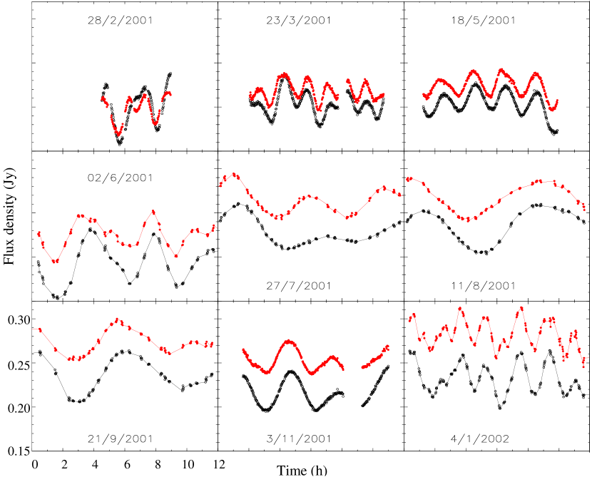
Figure 2 presents nine of the light curves at 4.8 and 8.6 GHz made at approximately six week intervals over the course of a year. Immediately apparent is the dramatic change in the time-scale of the flux density variations at both frequencies. From February through May, the flux density varies rapidly with less than one hour between excursions. In June the variations begin a slow down which lasts through September. November sees them speed up again, while by 2002 January they have returned to much the same rate as 2001 February. The time-scales estimated from the earlier discovery observations of 2000 June and September, and the more recent observations of 2002 February and April, are consistent with this annual cycle in the time-scale of variations. The annual cycle provides clear evidence that the observed rapid variations are due to interstellar scintillation (ISS). The change in the time-scale of variations through the year is due to the changing velocity of the scattering medium relative to the observer as the Earth revolves around the sun.
To quantify the observed changes we define a characteristic time-scale of variability. Various authors have used different definitions for characteristic time-scale of IDV sources. These are generally based upon estimates of either the auto-correlation function (ACF) or the structure function of the time series, or may be estimated from the time series itself. In studies of scintillation of pulsars, the usual convention is to define the time-scale as the lag at which the ACF falls to of its maximum value (Cordes, 1986). This definition of the “decorrelation time-scale”, , was adopted by Macquart & Jauncey (2002) in their paper on Earth Orbit Synthesis. Dennett-Thorpe & de Bruyn (2000A) define the time-scale by use of the structure function (e.g. Simonetti, Cordes, & Heeschen, 1985). Their definition of the variability time-scale corresponds to the full-width at of the ACF. Rickett et al. (1995) and Rickett, Kedziora-Chudczer & Jauncey (2002) define the time-scale as the half-width at half maximum of the ACF, which we call , and which is in general slightly smaller than .
For extragalactic sources, in addition to the above, several other “counting” parameters have been used in the literature. This is possible because the observed IDV is often quasi-sinusoidal, which leads to a deep minimum in the ACF, as shown in Figure 3. Kedziora-Chudczer et al. (1997) used the mean peak-to-peak time, while Jauncey & Macquart (2001) used the mean peak-to-trough or trough-to-peak time. While estimates from the ACF or structure function are more reliable, “counting” methods remain useful, particularly where the original data are unavailable.
We calculate the ACFs using the discrete correlation method and binning into time lag intervals (Edelson & Krolik, 1988), rather than interpolating the data. The discrete correlation method has the advantage that it is straight-forward to combine data from two (or more) consecutive days without interpolating across 12 hour gaps. The mean is first subtracted from each data point and the ACF is normalised to unity at zero lag. Specifically, the method is as follows. For each pair of data points we calculate the lag and the function , where is the flux density at time , is the mean flux density for the particular dataset, and is the corresponding variance of for the dataset. The elements are then binned according to lag, and the average is taken as the estimate of the ACF for each bin, provided a large number of elements lie within that bin. Figure 3 shows ACFs calculated from the data of 2001 March 23.
While choosing a definition for the time scale is a matter of convention, it is necessary to use a consistent method when comparing theoretical and observational results. For PKS 1257326 we have calculated various time-scale estimates for each frequency and for each dataset, and find, on average, that , applies over the whole year and at both frequencies. For direct comparison with the results of Rickett, Kedziora-Chudczer & Jauncey (2002) and Rickett et al. (1995), we choose to define the time-scale as , the 50% decay time of the ACF.
Figures and show determined for each session and at both frequencies plotted against day of year, and show quantitatively the remarkable annual cycle so apparent in Figure 2. Also included are the values calculated for the data from 2000, and the more recent observations of 2002 February, and April. The values for 2000 are plotted as limits. The light curve from June 2000 is somewhat undersampled and therefore gives an upper limit to , while the 2000 September data show a decrease in flux density over 4 hours, with a subsequent 4.5 hour gap in the data (due to observations for another project) followed by an increase over the next 3 hours, so we have only a lower limit on . Plotted in Figure is the expected scintillation speed vs day of year, assuming that the ISM is moving with the local standard of rest (LSR) (Rickett et al., 2001, and private communication). Figure displays the corresponding scintillation velocity projected onto the plane of the sky. Comparison of Figures and with Figure demonstrates that the phasing of the annual cycle closely matches the Earth’s projected speed with respect to the LSR. The annual cycle in is a result of the changing velocity of the scintillation pattern across the observer’s line-of-sight, and leaves no doubt as to the origin of the intra-day variability in this source. Such an annual cycle has been seen in two other sources; 0917624 (Rickett et al., 2001; Jauncey & Macquart, 2001), and J18193845 (Dennett-Thorpe & de Bruyn, 2001), and is expected if the IDV is in fact a propagation effect caused by a relatively local Galactic “screen”. To reflect the ISS nature of the rapid variations, we hereafter refer to the characteristic time-scale, estimated as the 50% decay time of the ACF, as .
Scintillation is a stochastic process, and since our observations sample this process over a finite duration, it is only possible to obtain an approximation to the true time-scale of the underlying process. This stochastic process, and our lack of understanding of it, are by far the dominant contributions to the uncertainty in any determination of the scintillation time-scale, . The uncertainty decreases with the number of independent samples of the scintillation pattern, or “scintles”, observed.
To estimate the error empirically, we divided the datasets from 12 well-sampled epochs, when is short and/or the dataset extends over two consecutive days, into subsets, and calculate for each subset. We assume that the statistical error due to the finite number of samples of the stochastic process scales as , where is the number of independent samples. We define in this case as , where is the length of the observation. We then assume that the fractional error, , is proportional to . For each subset we calculate , where the arises because the two estimates are not independent. From the observed distribution of , we estimate the fractional errors to be at 4.8 GHz, and at 8.6 GHz. The resultant error bars are shown in Figures and .
To evaluate the reliability of the above error estimates, we assume that is constant between day of year 50 and day of year 150 (late February through May), an assumption supported by the data in Figure 4, and by the almost constant value of (for a medium moving with the LSR, as shown in Figure 4) over this period. The observed rms scatter in the 8 data points from this period is 12% at 4.8 GHz and 19% at 8.6 GHz, compared with the mean of the errors determined for these data as above, of 13% at 4.8 GHz and 15% at 8.6 GHz. This indicates that our error estimates, as derived above, are reasonable.
Figure 2 also shows that the IDV at 4.8 and 8.6 GHz remained strongly correlated over 12 months of these observations; in fact we have observed correlated variability between the two frequencies in every observation since the discovery of IDV in 2000 June. The increasing difference between the mean flux density levels reveals that the spectral index became increasingly inverted as the mean flux density at 8.6 GHz increased by 70%, while that at 4.8 GHz increased by 35%. This is clearly seen in Figures and , which show all data from well-sampled epochs at both frequencies, and Figure , which shows the mean spectral index at each epoch. The source appears to be undergoing a pc-scale “outburst” of the type commonly seen in many flat-spectrum AGN (e.g., Kellermann & Pauliny-Toth, 1968).
Figure shows that despite the increase in total flux density, there is little evidence for a systematic increase or decrease of the rms variations at either frequency. If the increase in flux density were due to an increase in the flux density of the scintillating component, we would expect to see either a large increase in the rms variations, or if the scintillating component were expanding, we may observe an increase in the characteristic time-scale (in addition to the annual cycle). However, neither has been observed. Regression analysis shows that there is at best a very weak correlation in the sense that there may be a slight increase with time of the rms variations at 8.6 GHz. Given the low significance of this result, we are continuing to monitor the variations at both frequencies to look for any change in the scintillation behaviour. The connection between ISS and intrinsic variability is further discussed in Section 4.
Finally, close inspection of Figure 2 reveals that at each epoch, the 8.6 GHz variability pattern appears to lead the 4.8 GHz light-curve. The time delay between the variations at the two frequencies, , was quantified by cross-correlating the 4.8 and 8.6 GHz observations at each epoch. Although the overall variability patterns at both frequencies are quite similar, there is some extra “structure” in the 8.6 GHz light curves which appears to be more smoothed in the 4.8 GHz light curves. Therefore only light curves with well-sampled peaks and troughs give a reliable time delay measurement. As shown in Figure 6, the peak of the cross-correlation always has the same sign, i.e. the 8.6 GHz variations are leading. Although the uncertainty in each individual measurement is large, due to limited sampling and the fact that the light curves at each frequency are not identical, this result is significant. Interestingly, there is a clear correlation of with the inverse of the predicted ISM velocity (Figure ). This gives a second annual cycle in the variability of this unusual source. In the next section we examine in detail the implications of these results for PKS 1257326 and the ISM in our line-of-sight to this source.
3 Microarcsecond Source Structure
The clear presence of an annual cycle in the time-scale of variability identifies interstellar scintillation as the mechanism responsible for the IDV in PKS 1257326, which in turn allows a determination of both source and scattering screen properties. Over the course of a year, the Earth’s orbital motion produces changes in both the magnitude and direction of the net scintillation velocity, , which both potentially contribute to changes in . Figure shows the Earth’s velocity relative to the LSR over the course of a year, projected onto the plane transverse to the source line-of-sight. If the scintillation pattern is isotropic, only the change in the nett scintillation speed contributes to variations in . In this case, the observed is inversely proportional to . However, the length scale of the scintillation pattern may change with orientation, in which case will also change as the direction of changes. An elongated scintillation pattern could be produced by elongated source structure and/or by anisotropic scattering in the ISM.
Rickett, Kedziora-Chudczer & Jauncey (2002) showed that the deep first minimum, which they term a negative “overshoot”, in the ACFs for data on PKS 0405385 during its episode of fast scintillation, indicates that the scattering is highly anisotropic. Their results from numerical simulation suggest that the scintillation pattern of PKS 0405385 has an axial ratio of 0.25 or less, where is approximately aligned with the short axis of the irregularities. For more highly anisotropic irregularities, the depth of the ACF first minimum does not change significantly. The negative overshoot is a measure of the spectral purity of the fluctuations: the closer to sinusoidal the variations are, the closer to is the depth of the first minimum in the ACF. Rickett, Kedziora-Chudczer & Jauncey (2002) argue that the negative overshoot is an effect of anisotropic scattering in the ISM, and cannot be duplicated by anisotropic source structure.
A large number of independent samples of the scintillation pattern are required to determine a reliable ACF. For light curves which sample only 1 or 2 scintles, the ACF is poorly determined and thus a spurious negative overshoot can occur. For all of the long datasets on PKS 1257326, the average depths of the first minima in the normalized ACFs are () and (), at 4.8 GHz and 8.6 GHz respectively. Assuming that the model of Rickett, Kedziora-Chudczer & Jauncey (2002) applies to PKS 1257326, this indicates that the scattering is anisotropic, with the minor axis of the scintillation pattern aligned within of the plasma velocity vector. The minima at 4.8 GHz are, on average, deeper than at 8.6 GHz, although there is substantial scatter (for example, Figure 3 shows that for the 2001 March 23 data, the first minimum of the ACF was in fact deeper at 8.6 GHz.) The fact that the average size of the “negative overshoot” differs at each frequency may be a result of a differing source size relative to the Fresnel scale, i.e. the 8.6 GHz component may have a larger ratio of angular source size to angular size of the first Fresnel zone, , than the 4.8 GHz component. Hence the negative overshoot in the ACF could be suppressed at 8.6 GHz as source size effects become more important.
Our data indicate that the scintillations observed at 4.8 and 8.6 GHz are in the regime of weak scattering, where the medium introduces a phase change of less than 1 radian across a Fresnel zone (e.g. Walker, 1998). Correlated variability between 4.8 and 8.6 GHz is a pattern commonly seen in other IDV sources at high Galactic latitudes, in particular the other extreme IDVs. At lower frequencies, is generally much longer and the variability is not correlated with the higher frequency variability. This is explained in terms of weak and strong scattering. At 4.8 and 8.6 GHz, the sources undergo weak scintillations, while lower frequencies (below GHz) are in the regime of strong (refractive) scattering (e.g. Kedziora-Chudczer et al., 1997; Walker, 1998). Time-scales of variability for refractive scintillations increase with wavelength, , as .
In the regime of weak scattering, the typical length scale of the scintillations is equal to the Fresnel scale, , where is the distance to the scattering plasma and is the observing frequency. The Fresnel scale sets an effective cut-off diameter for the angular size of a source undergoing weak scintillation, . A source this size or smaller exhibits flux density variations on a time-scale , where vISS is the speed of the scattering material across the line of sight. For larger source sizes, , the scintillations decrease in amplitude as and increase in timescale as (e.g. Rickett, 2002). It may be that AGN have a sufficiently large angular diameter that the source size influences the observed scintillation pattern. Another effect of larger source sizes is that scintillations from distant scattering material are suppressed, since the angular size “cut-off”, set by the first Fresnel zone, scales as . Therefore, there will be a bias towards finding sources that scintillate behind nearby ISM turbulence.
We can use our measurements of the annual cycle in to constrain (i) the velocity of the scattering medium, (which Figure 4 suggests is not very different from the LSR), (ii) the source angular size, , and (iii) the distance to the scattering screen, . The parameters used to model the observed annual cycle in are as follows. may be offset from the LSR and this introduces two free parameters, the components of this offset in the plane transverse to the source line-of-sight. As shown in Figure 4d, the projected velocity of the sun with respect to the LSR in RA and Dec components is v km s-1, v km s-1. The RA and Dec offsets, and , of the components shift the origin in Figure . Two more parameters are required to describe the axial ratio and orientation of anisotropy in the scintillation pattern. Finally there is an overall scaling factor, , which sets the scintillation length scale. We choose to be the minor axis of the scintillation pattern. We have tested the effect of varying these parameters, and find that the shape of the resulting annual cycle is quite sensitive to variations in the ISM velocity and the angle of the elongation for an anisotropic scintillation pattern. We find the best fit parameters at each frequency by minimising the sum of squares of the residuals. We have examined fits both for the case of unweighted residuals, and for the case of residuals weighted by the error associated with each point. The shape of the slow-down period is critical in determining the ISM velocity and anisotropy in the scintillation pattern. However the errors in are larger in this period, due to having fewer independent samples of the scintillation pattern. By using the unweighted residuals (i.e. ignoring the errors) we allow the fit to be better constrained by these points in the slow-down period. On the other hand, the overall scintillation length-scale is more accurately estimated using the better-sampled data from the fast period. We find that for models which fit the data well, using weighted or unweighted residuals makes little difference to the results.
If we assume isotropic scattering and an isotropic source, the best fit to the peak in is achieved with km s-1 and km s-1 at 4.8 GHz, where and negative have the effect of moving the origin in Figure 4 further away from the ellipse. At 8.6 GHz the best fit is for km s-1 and km s-1. Assuming the same scattering material is responsible for the scintillation at both frequencies, we take the average as the overall best fit: km s-1 and . These fits, and fits for several other velocity offsets, are shown in Figures and . The scintillation length-scale, , is a function of and . While we expect that source size influences the scintillation in PKS 1257326, at least to the extent that scintillations from more distant scattering material are suppressed, the size of the scintillating component, , cannot be very much larger than the Fresnel scale at the distance of the scattering plasma, otherwise the source would not show such deep modulations in flux density. The average ratio of at the two frequencies is which is consistent with being equal to Therefore the source size may in fact be smaller than, or equal to, the Fresnel scale at both frequencies. Alternatively, the source size may scale with frequency in a similar way, i.e. . To consider both possibilities, we introduce a scaling parameter
and approximate the scintillation length scale as . Thus
| (1) |
Because , uncertainties in lead to greater uncertainties in , and the screen distance is rather weakly constrained. For the isotropic case, the allowable range of values found for the scintillation length-scale are km at 4.8 GHz, and km at 8.6 GHz. Letting (i.e. ) gives an approximate upper limit on . Inserting these values we find pc at 4.8 GHz, and pc at 8.6 GHz. This implies that the scattering occurs in a very local region of turbulence, as has been suggested for the other two intra-hour scintillators, J1819+3845 (Dennett-Thorpe & de Bruyn, 2000A) and PKS 0405385 (Rickett, Kedziora-Chudczer & Jauncey, 2002). If , this implies an even closer screen. For a distance in the range 10–15 pc, corresponds to an angular size in the range 30–37 as at 4.8 GHz, and 22–28 as at 8.6 GHz.
To obtain limits on the source brightness temperature, , we also need to know the flux density, , of the scintillating component of PKS 1257326. Following the arguments of Rickett, Kedziora-Chudczer & Jauncey (2002), cannot be more than the total average flux density and cannot be negative, so we have , where is the total average flux density and is the lowest flux density observed. Since we know varies with time, we compute for each epoch, and find that the maximum value is close to 50 mJy at both frequencies. Also, at the start of our monitoring was mJy at both frequencies. In fact we can place a further constraint on at 4.8 GHz, since a short-baseline VLBI observation of the source, including the ATCA and an unresolved calibrator to set the flux density scale, showed that % of the total average flux of PKS 1257326 (on 2001 March 23) is missing on an angular scale of at 4.8 GHz. Thus we assume 50 mJy 150 mJy.
Assuming a circularly symmetric source brightness distribution with FWHM corresponding to the Fresnel scale size, an approximate lower limit on the rest-frame brightness temperature, K, is obtained for mJy and as at an observed frequency of 4.8 GHz. This requires relativistic beaming with a Doppler factor of so as not to violate the Inverse Compton (IC) limited brightness temperature of K for synchrotron radiation. If in the rest frame the source is at an equipartition brightness temperature of K, as defined by Readhead (1994), then is required. While high, these implied Doppler factors are not inconsistent with apparent superluminal speeds found in VLBI surveys (Marscher et al., 2000; Kellermann et al., 2000). Taking mJy and as gives a somewhat more extreme brightness temperature of K.
Figures and show fits obtained allowing an anisotropic scintillation pattern with no velocity offset from the LSR. As discussed above, there is independent evidence for anisotropic scattering, based on the depth of the first minimum in the ACFs. Finally, Figures and show fits obtained for an anisotropic scintillation pattern and allowing a screen velocity offset from the LSR. The width of the peak, allowing all parameters to vary, is best fitted for both frequencies with km s-1 and , and when the minor axis of the scintillation pattern lies at an angle of approximately to . The ISM velocity offset is shown by the arrow in Figure 4, and the orientation of the fitted scintillation pattern is shown by the small ellipse in Figure 4. The best fits are found for axial ratios . Decreasing the axial ratio below has little effect on the shape of the annual cycle, because never cuts directly across the long axis of the fitted scintillation pattern. This result is consistent with what is expected from depth of the first minimum in the ACFs, which in the case of PKS 0405385 was fitted with a highly anisotropic medium (axial ratio ; Rickett, Kedziora-Chudczer & Jauncey 2002). Those sources for which at its maximum cuts across the short axis of the scintillation pattern are those most likely to scintillate rapidly.
For the best fits allowing all parameters to vary, the minor axes of the scintillation pattern scale are approximately km at 4.8 GHz, and km at 8.6 GHz. In the case of anisotropic scattering, the typical length scale for the minor axis is the Fresnel scale reduced by a factor of (B.J. Rickett 2002, priv. comm.). We estimate by setting and replacing with in Equation 1. This gives values for the screen distance of pc at 4.8 GHz, and pc at 8.6 GHz; very similar values to those obtained for the isotropic case. Hence the implied brightness temperatures are also very similar to those found for the case of an isotropic scintillation pattern. However, in the case of anisotropic scattering, it may be that could be reduced further if the source was coincidentally elongated in the same direction as the long axis of the scattering.
For rapid scintillators such as PKS 1257326, it is possible to measure the IDV pattern time delay between two widely separated telescopes (Jauncey et al., 2000; Dennett-Thorpe & de Bruyn, 2002). Recently we observed PKS 1257326 simultaneously using the ATCA and the Very Large Array (VLA), and observed a clear time delay between the IDV pattern arrival times at each telescope (Bignall et al., in preparation). By measuring this delay 2 or 3 times over the course of a year, we will obtain an accurate, independent estimate of the scintillation parameters.
3.1 Annual cycle in the time offset between 4.8 and 8.6 GHz
We now turn our attention to the annual cycle in , the offset between the IDV patterns observed at 4.8 and 8.6 GHz. We suggest that this may be due to an offset between the central components of the source at each frequency, as might be expected if the source were jet-like on a as scale, and optically thick between 5 and 8 GHz. The line in Figure 6 shows an expected annual cycle for an offset between the two components, with projected displacement vector km in components of RA and Dec, using the best-fit ISM velocity derived from the annual cycle above. Given the large (but difficult to estimate) uncertainties in the measurement of , this model seems a reasonable fit to the data. The fact that always has the same sign means that the ISM always crosses the 8.6 GHz “component” first, which severely constrains the direction of the offset of the two components, and also implies that the origin in Figure cannot be inside the ellipse; i.e. changes direction by over the year. This is consistent with what is expected from the annual cycle in .
For a screen distance of 10 pc, the fitted displacement vector corresponds to an offset of as. This order of resolution is currently unachievable by any other technique, and is comparable to that expected for proposed future space-based X-ray (Cash et al., 2000) and optical (Unwin et al., 2002) interferometry missions. An offset of this order between different frequency components may also have implications for future astrometry and geodesy programs. An angular scale of as at corresponds to a linear scale of 0.08 pc.
Another possibility which we have not ruled out is that the frequency offset is due to a refractive effect in the ISM rather than the source itself. Theoretical investigation of such effects is ongoing and will be presented in a later paper.
4 Discussion
The evidence for interstellar scintillation as the principal cause of IDV at cm wavelengths is now compelling. Three sources have shown a clear annual cycle in the changes in their characteristic time-scales, J18193845, 0917624, and now PKS 1257326. In addition, a time-delay has been measured in the arrival times of the IDV pattern at widely spaced radio telescopes for PKS 0405385 (Jauncey et al., 2000), J18193845 (Dennett-Thorpe & de Bruyn, 2002), and recently PKS 1257326 (Bignall et al., in preparation).
At this point, it is important to re-examine the evidence presented for an intrinsic origin for cm-wavelength IDV. The strongest case reported is the correlated radio-optical changes found in 0716714 (Quirrenbach et al., 1991; Wagner et al., 1996). In 1990 February, optical variations were found that were strongly correlated with changes in the radio spectral index between 6 and 3.6 cm wavelengths, in the sense that the optical flux increased as the radio spectrum became more inverted. If this correlation were to extend across the spectrum from radio to optical wavelengths, as would be the case if the changes were intrinsic, then such a spectral inversion should lead directly to even stronger flux density changes at wavelengths shorter than 3.6 cm. However, such changes are not evident in the 2 cm data for this source from the same epoch (Quirrenbach et al., 2000). This raises some doubt as to the value of the evidence for the intrinsic nature of the variability seen in this source in 1990 February. It is notable that 0716714 continues to show dramatic optical variability on a time-scale of days or less (Nesci, Massaro & Montagni, 2002).
Alternatively, the low level of IDV in 0716 at both 20 and 2 cm is consistent with a scintillation origin, as is seen in the variations in amplitude of IDV with frequency in both PKS 0405385 (Kedziora-Chudczer et al., 1997) and J18193845 (Dennett-Thorpe & de Bruyn, 2000A). Moreover, the apparent difference in phase between the 5 and 8 GHz data resembles that apparent in PKS 1257326, as well as in J18193845 (see figure 2 of Dennett-Thorpe & de Bruyn 2000A), further strengthening the case for a scintillation origin of the radio IDV in 0716714. Given its proximity on the sky to 0917624, it is important to search for an annual cycle in the variability time-scale of this source, similar to that seen in 0917624 (Rickett et al., 2001; Jauncey & Macquart, 2001).
The case for interstellar scintillation at cm-wavelengths is so strong that we suggest that this phenomenon be referred to as the physical phenomenon of interstellar scintillation, rather than the observational phenomenon of IDV. This is not merely a change in nomenclature, but has value in focusing on the physics; while IDV is scintillation, scintillation is not necessarily IDV. For example, in the strong (refractive) scattering regime, scintillating sources show a characteristic time-scale which increases with decreasing frequency (), that is easily an order of magnitude or more longer than intra-day.
What is the connection, then, between scintillation and intrinsic variability at cm wavelengths? Variability of compact, flat-spectrum radio sources has been studied in detail for four decades. These sources often show large “outbursts” on time-scales of months to years at cm wavelengths, which have been successfully modelled as intrinsic variations in relativistic jets, and linked with apparent superluminal motions of components observed with VLBI (e.g. Kellermann & Pauliny-Toth, 1981). While refractive scintillations were found to be important for low frequency variability (frequencies GHz) (Hunstead, 1972; Rickett, Coles, & Bourgois, 1984), for many years the prevailing paradigm was that cm wavelength variability was all intrinsic. It was only with the discovery of rapid IDV (e.g. Kedziora-Chudczer et al., 1997) implying excessively high brightness temperatures if the variability was intrinsic ( K in the case of PKS 0405385), that the importance of ISS at cm wavelengths has been extensively re-examined. In particular, the largest intensity fluctuations due to ISS are observed at frequencies close to the transition between weak and strong scattering, typically GHz along lines of sight out of the Galactic plane (Walker, 1998).
Our flux density monitoring of PKS 1257326 suggests that it is also undergoing the type of intrinsic, pc-scale outburst commonly seen in flat-spectrum sources, yet there has been no significant change in the scintillating flux density. This is despite the optically thick spectrum of the slowly varying source, and suggests that the as core does not lie behind what is presumably an expanding pc-scale jet, as might be expected if the scintillating component were the core at the base of the pc-scale jet. In other words, the outburst is probably occurring in a separate emitting region, further out from the core in a component too large to scintillate. High resolution VLBI observations could provide information on activity in the source on a scale of several pc.
It is interesting to compare the brightness temperature inferred from the long-term intrinsic variability, with that obtained from the ISS model. For PKS 1257326, we observed a steady increase in the mean flux density at 8.6 GHz of Jy over a period of 440 days, while over the same time the mean 4.8 GHz flux density increased by Jy. The simple approach of taking these values of to be the flux density of the slowly varying component at each frequency, and observed variability time-scale days, gives a variability brightness temperature (in the source proper frame), , of K from the 8.6 GHz long-term variability, and K from the 4.8 GHz long-term variability (Lähteenmäki & Valtaoja, 1999). For relativistically beamed radiation with Doppler factor , the inferred variability brightness temperature is related to the source rest-frame brightness temperature , by . Where is calculated from an angular size which has been measured directly, or estimated from an ISS model as in Section 3 above, then . Taking this dependence into account, the intrinsic brightness temperature inferred from the long-term variability is smaller than that calculated from the modelled angular size of the scintillating component. This is consistent with the long-term variability occurring in a larger region, separate from the scintillating component, and the lack of any detectable change in the scintillating flux density.
In some sources, variability due to ISS is episodic. For example, the IDV in PKS 0405385 has been convincingly shown to be due to ISS (Kedziora-Chudczer et al., 1997; Jauncey et al., 2000; Rickett, Kedziora-Chudczer & Jauncey, 2002), however this source has shown only short-lived episodes of fast scintillation, each lasting several months (Kedziora-Chudczer et al., 2001B). PKS 0405385 also exhibits slow flux density evolution, and Kedziora-Chudczer et al. (1997) proposed a possible interpretation of the episodic ISS, relating the long-term behaviour to the ejection and subsequent expansion of a component small enough to scintillate. However, this interpretation did not agree so well with the second episode of ISS observed in 1998, and it remains unclear whether the transient nature of the scintillation observed in PKS 0405385 is due to intrinsic changes in the source occurring on time-scales of months, which cause the appearance and disappearance of a scintillating component, or to changes in the properties of the scattering medium.
A similar problem exists for 0917624. Recent monitoring data on this source were presented at the AGN Variability Workshop in Sydney by Fuhrmann et al. (2002), showing that the rapid, large-amplitude scintillation of this source has recently ceased after 15 years of monitoring. More recent VLA data collected during the MASIV Survey (Lovell et al., in preparation), and data from the Goldstone–Apple Valley Radio Telescope program (M. Klein, priv. comm.) confirm that the rapid scintillations in 0917624 have so far not returned.
While ISS and observations of annual cycles are useful for probing as-scale source structure, there is clearly much remaining to be understood about ISS of extragalactic radio sources, and its connection to the intrinsic variability which generally occurs on longer time-scales.
5 Significance of the Fast Scintillators
The three fast scintillators PKS 0405385, J18193845, and PKS 1257326, are valuable because their rapid scintillation time-scale allows one to characterize the statistics of the underlying scintillation process over a typical 12-hour observing session; one observes more stastically independent “scintles” per unit time compared with slower scintillators. This is important because the dominant source of error in modelling the structure of a scintillating source is in the stochastic properties of the scintillation process itself. Moreover, in their periods of rapid variability it proved possible to make the pattern time delay measurements, crucial in establishing the ISS origin (Jauncey et al., 2000; Dennett-Thorpe & de Bruyn, 2002), since this is not possible for the more usual, slower scintillating sources with characteristic time scales of order a day. These three rapidly scintillating sources proved invaluable in making the transition from IDV to ISS. Viewed from an IDV perspective, their properties appear extreme. From a scintillation perspective, however, are these sources really so extreme?
The answer lies in the reasons for their rapid scintillation. The characteristic time-scale for scintillation is , where is the scintillation length scale and is the bulk velocity of the scattering plasma in the observer’s frame of rest. If an annual cycle is observed in , it follows that the scattering plasma velocity must be close to the 30 km s-1 of the Earth’s orbital speed. As discussed in Section 3, for an observed frequency in the weak scattering regime, is related to the Fresnel scale, , which scales with screen distance as . also depends on the source angular size, , in the case where this exceeds the angular Fresnel scale, such that . For most extragalactic sources, the relation of time scale to screen distance lies between a square root and a linear dependence (Rickett, Kedziora-Chudczer & Jauncey, 2002). It follows that the fast scintillators, those with small , will be those scintillating sources which are to be found behind very nearby scattering screens. The evidence in support of this is the screen distances of pc found for J18193845 (Dennett-Thorpe & de Bruyn, 2000A), PKS 0405385 (Rickett, Kedziora-Chudczer & Jauncey, 2002), and PKS 1257326.
From the scintillation perspective, these fast variables are extreme in the sense that they are to be found behind nearby scattering material, not in that there is any inherently extreme property in the sources themselves. There is no evidence for anything intrinsically unusual about PKS 1257326 which sets it apart from other flat-spectrum, radio-loud quasars. It has optical magnitude and has been detected at X-ray energies, emitting erg cm-2 s-1 between 0.1 and 2.0 keV (Perlman et al., 1998). In fact, its radio properties are less extreme than might be expected for the more common, slower scintillators. Since the angular size required for a source to scintillate in the ISM is set by the angular size of the first Fresnel zone, those sources which show large variations with longer characteristic time scales are more likely to be found behind scattering screens at much larger distances, and hence with smaller angular sizes and correspondingly higher brightness temperatures.
There are also implications for the properties of the interstellar medium. The small number of fast scintillators suggests that there are few regions of the Galaxy where such nearby screens may be found, a point supported by the observation that the screen towards J18193845 does not move at the local standard of rest (Dennett-Thorpe & de Bruyn, 2002). Moreover, as noted above, the presence of a nearby screen relaxes the constraints on the angular size necessary for a source to scintillate. Thus there will likely be more sources with components with angular sizes of order 20 as, which can scintillate through a screen at pc, than there will be sources with 5–10 as angular sized components to scintillate through a screen at, say, 500 pc. In this regard, it is noticeable that the two long-lived fast scintillators, J18193845 and PKS 1257326, are the two weakest IDV sources reported. If the above is correct, then a deep, unbiased scintillation survey would be expected to confirm the low numbers of fast scintillators. Alternatively, the discovery of more such rapid scintillators can reveal the presence of such nearby scattering material in the Galaxy. A survey is currently underway, using the VLA to look for scintillation-induced variability over the whole Northern sky, in both strong ( Jy) and weak ( Jy) flat-spectrum sources (Lovell et al., in preparation).
6 Summary
Here we summarize the main results from our observations of PKS 1257326.
- •
-
•
Monitoring over more than a year reveals a clear annual cycle in the characteristic timescale of variability.
-
•
This annual cycle provides unequivocal evidence for a scintillation origin of the IDV observed in this source.
-
•
Modelling the annual cycle provides strong evidence for highly anisotropic scattering in the ISM.
-
•
The very rapid variability is most likely due to scintillation in a nearby screen, only to 15 pc from the sun.
-
•
Assuming a source size equal to the Fresnel scale at the distance of the screen, the implied brightness temperature is then K, which is high, but not entirely unacceptable for relativistically beamed radiation from a jet.
-
•
A time offset is observed between the scintillation patterns at each frequency, which itself exhibits an annual cycle. This we tentatively model as an offset due to opacity effects in the source on a scale of as, or pc at the source.
-
•
There are much slower flux density changes in the pc-scale structure of the source, but these do not appear to be mirrored in any obvious changes in the microarcsecond sized component responsible for the IDV.
-
•
We plan to continue to monitor PKS 1257326, to better constrain the time-scale during the slow-down period, and to follow pc-scale changes in the source with high-resolution VLBI observations.
-
•
For sources scintillating in the weak scattering regime which show large variations on timescales of the order of a day, the scattering screens may be at much larger distances (several hundred pc). This requires smaller source sizes, so in fact these slower scintillators may have higher implied brightness temperatures than the very rapid scintillators.
-
•
Observations of scintillating sources provide a method of achieving as resolution at cm-wavelengths with modest radio telescopes, resolution comparable with that proposed for future space-based optical and X-ray interferometers.
References
- Bignall et al. (2002) Bignall, H. E., Jauncey, D. L., Kedziora-Chudczer, L., Lovell, J. E. J., Macquart, J. P., Rayner, D. P., Tingay, S. J., Tzioumis, A. K., Clay, R. W., Dodson, R. G., McCulloch, P. M., & Nicolson, G. D. 2002, PASA, 19, 29
- Burbidge, Jones, & Odell (1974) Burbidge, G. R., Jones, T. W., & Odell, S. L. 1974, ApJ, 193, 43
- Cash et al. (2000) Cash, W., Shipley, A., Osterman, S., & Joy, M. 2000, Nature, 407, 160
- Cordes (1986) Cordes, J. M., 1986, ApJ, 311, 183
- Dennett-Thorpe & de Bruyn (2000A) Dennett-Thorpe, J. & de Bruyn, A. G. 2000A, ApJ, 529, L65
- Dennett-Thorpe & de Bruyn (2000B) Dennett-Thorpe, J. & de Bruyn, A. G. 2000B, in IAU Symposium 205, ed. Schilizzi, R. T. et al. (San Francisco:ASP), 88
- Dennett-Thorpe & de Bruyn (2001) Dennett-Thorpe, J. & de Bruyn, A. G. 2001, Ap&SS, 278, 101
- Dennett-Thorpe & de Bruyn (2002) Dennett-Thorpe, J. & de Bruyn, A. G. 2002, Nature, 415, 57
- Edelson & Krolik (1988) Edelson, R. A. & Krolik, J. H. 1988, ApJ, 333, 646
- Fuhrmann et al. (2002) Fuhrmann, L., Krichbaum, T. P., Cimò, G., Beckert, T., Kraus, A., Witzel, J. A., Qian, S. J., & Rickett, B. J. 2002, PASA, 19, 64
- Heeschen (1984) Heeschen, D. S. 1984, AJ, 89, 1111
- Heeschen et al. (1987) Heeschen, D. S., Krichbaum, T. P., Schalinski, C. J., & Witzel, A. 1984, AJ, 89, 1111
- Hunstead (1972) Hunstead, R. W. 1972, Astrophys. Lett., 12, 193
- Jauncey et al. (2000) Jauncey, D. L., Kedziora-Chudczer, L., Lovell, J. E. J., Nicolson, G. D., Perley, R. A., Reynolds, J. E., Tzioumis, A. K., & Wieringa, M. H. 2000, in Astrophysical Phenomena Revealed by Space VLBI, ed. H. Hirabayashi, P. G. Edwards & D. W. Murphy (Sagamihara:ISAS), 147
- Jauncey et al. (2001) Jauncey, D. L., Kedziora-Chudczer, L., Lovell, J. E. J., Macquart, J.-P., Nicolson, G. D., Perley, Rick A.; Reynolds, J. E., Tzioumis, A. K., Wieringa, M. H., Bignall, H. E. 2001, Ap&SS, 278, 87.
- Jauncey & Macquart (2001) Jauncey, D. L., & Macquart, J.-P. 2001, A&A, 370, L9
- Kedziora-Chudczer et al. (1997) Kedziora-Chudczer, L., Jauncey, D. L., Wieringa, M. H., Walker, M.A., Nicolson, G. D., Reynolds, J. E., & Tzioumis, A. K. 1997, ApJ, 490, L9
- Kedziora-Chudczer et al. (2001A) Kedziora-Chudczer, L., Jauncey, D. L., Wieringa, M.H., Tzioumis, A. K., & Reynolds, J. E. 2001A, MNRAS, 325, 1411
- Kedziora-Chudczer et al. (2001B) Kedziora-Chudczer, L., Jauncey, D. L., Wieringa, M. A., Tzioumis, A. K., & Bignall, H. E. 2001B, Ap&SS, 278, 113
- Kellermann & Pauliny-Toth (1968) Kellermann, K. I., & Pauliny-Toth, I. I. K. 1968, ARA&A, 6, 417
- Kellermann & Pauliny-Toth (1981) Kellermann, K. I., & Pauliny-Toth, I. I. K. 1981, ARA&A, 19, 373
- Kellermann et al. (2000) Kellermann, K. I., Vermeulen, R. C., Zensus, J. A., & Cohen, M. H. 2000, in Astrophysical Phenomena Revealed by Space VLBI, ed. H. Hirabayashi, P. G. Edwards & D. W. Murphy (Sagamihara:ISAS), 159
- Lähteenmäki & Valtaoja (1999) Lähteenmäki, A. & Valtaoja, E. 1999, ApJ, 521, 493
- Lovell et al. (in preparation) Lovell, J. E. J., Jauncey, D. L., Bignall, H. E., Kedziora-Chudczer, L., Macquart, J.-P., Rickett, B. J., & Tzioumis, A. K., ‘First Results from MASIV: The Micro-Arcsecond Scintillation-Induced Variability Survey’, in preparation.
- Macquart et al. (2000) Macquart, J.-P., Kedziora-Chudczer, L., Rayner, D. P., & Jauncey, D. L. 2000, ApJ, 538, 623
- Macquart & Jauncey (2002) Macquart, J.-P., & Jauncey, D. L. 2002, ApJ, 572, 786
- Marscher et al. (2000) Marscher, A. P., Marchenko-Jorstad, S. G., Mattox, J. R., Wehrle, A. E., & Aller, M. F. 2000, in Astrophysical Phenomena Revealed by Space VLBI, ed. H. Hirabayashi, P. G. Edwards & D. W. Murphy (Sagamihara:ISAS), 39
- Nesci, Massaro & Montagni (2002) Nesci, R., Massaro, E. & Montagni, F., PASA, 19, 143
- Perlman et al. (1998) Perlman, E., Padovani, P., Giommi, P., Sambruna, R., Jones, L. R., Tzioumis, A., & Reynolds, J. 1998, ApJ, 115, 1253
- Quirrenbach et al. (1991) Quirrenbach, A., Witzel, A., Wagner, S., Sanchez-Pons, F., Krichbaum, T. P., Wegner, R., Anton, K., Erkens, U., Haehnelt, M., Zensus, J. A., & Johnston, K. J. 1991, ApJ, 372, L71
- Quirrenbach et al. (2000) Quirrenbach, A., Kraus, A., Witzel, A., Zensus, A.J., Peng, B., Krichbaum, T. P., Wegner, R., and Naundorf, C.E. 2000, A&AS, 141, 221
- Readhead (1994) Readhead, A. C. S. 1994, ApJ, 426, 51
- Reynolds (1994) Reynolds, J. E. 1994, ATNF Technical Document Series 39.3/040, Australia Telescope National Facility
- Rickett, Coles, & Bourgois (1984) Rickett, B. J., Coles, W. A., & Bourgois, G. 1984, A&A, 134, 390
- Rickett et al. (1995) Rickett, B. J., Quirrenbach, A., Wegner, R., Krichbaum, T. P., & Witzel, A. 1995, A&A, 293, 479
- Rickett et al. (2001) Rickett, B. J., Witzel, A., Kraus, A., Krichbaum, T.P., & Qian, S.J. 2001, ApJ, 550, L11
- Rickett (2002) Rickett, B. J. 2002, PASA, 19, 100
- Rickett, Kedziora-Chudczer & Jauncey (2002) Rickett, B. J., Kedziora-Chudczer, L. and Jauncey, D. L. 2002, ApJ, in press
- Simonetti, Cordes, & Heeschen (1985) Simonetti, J. H., Cordes, J. M. and Heeschen, D. S. 1985, ApJ, 296, 46
- Unwin et al. (2002) Unwin, S. C., Wehrle, A. E., Jones, D. L., Meier, D. L., & Piner, B. G. 2002, PASA, 19, 5
- Wagner & Witzel (1995) Wagner, S. J., & Witzel, A. 1995, ARA&A, 33, 163
- Wagner et al. (1996) Wagner, S. J., Witzel, A., Heidt, J., Krichbaum, T.P., Quirrenbach, A., Wegner, R., Aller, H., Aller, M., Anton, K., Appenzeller, I., Eckart, A., Kraus, A., Naundorf, C., Kneers, R., Steffen, W., & Zensus, J. A. 1996, AJ, 111, 2187
- Walker (1998) Walker, M. A. 1998, MNRAS, 294, 307
- Witzel et al. (1986) Witzel, A., Heeschen, D. S., Schalinski C. J., & Krichbaum, T. P. 1986, Mitt. Astron. Ges., 65, 239